Article

Enhancing Seasonal PM2.5 Estimations in China through Terrain–Wind–Rained Index (TWRI): A Geographically Weighted Regression Approach

1
School of Geosciences and Info-Physics, Central South University, Changsha 410083, China
2
Laboratory of Geohazards Perception, Cognition and Predication, Central South University, Changsha 410083, China
*
Author to whom correspondence should be addressed.
Remote Sens. 2024, 16(12), 2145; https://doi.org/10.3390/rs16122145
Submission received: 24 April 2024 / Revised: 8 June 2024 / Accepted: 10 June 2024 / Published: 13 June 2024

Abstract

:
PM2.5 concentrations, closely linked to human health, are significantly influenced by meteorological and topographical factors. This study introduces the Terrain–Wind–Rain Index (TWRI), a novel index that integrates the Terrain–Wind Closed Index (TWCI) with relative humidity to quantitatively examine the coupling effect of natural elements on PM2.5 concentration and its application to PM2.5 inversion. By employing Geographically Weighted Regression (GWR) models, this study evaluates the inversion results of PM2.5 concentrations using TWRI as a factor. Results reveal that the annual average correlation between TWRI and site-measured PM2.5 concentrations increased from 0.65 to 0.71 compared to TWCI. Correlations improved across all seasons, with the most significant enhancement occurring in summer, from 0.51 to 0.66. On the inversion results of PM2.5, integrating TWRI into traditional models boosted accuracy by 1.3%, 5.4%, 4%, and 7.9% across four seasons, primarily due to the varying correlation between TWRI and PM2.5. Furthermore, the inversion results of coupled TWRI more effectively highlight the high value areas in closed areas and the low value areas in humid areas.

1. Introduction

The atmosphere is one of the fundamental elements that humans rely on for survival and development [1,2]. Emerging studies have shown that long-term exposure to air pollutants, particularly PM2.5, increases the risk of respiratory and cardiovascular diseases [3,4,5]. PM2.5 primarily originates from human activities and is influenced by meteorological conditions [6,7,8]. Sources of PM2.5 primarily include human activities such as industrial operations, agriculture, and transportation [9,10], with concentrations also being influenced by natural meteorological factors like wind speed, relative humidity, terrain, and planetary boundary layer, etc. [6,11,12]. Despite significant economic progress, China faces severe air pollution, with PM2.5 being a significant concern [13,14]. In response to this issue, China initiated the nationwide air quality monitoring in 2013 to monitor air pollutants in real-time. However, the network, with uneven and sparse spatial distribution, cannot meet the requirements of high spatial and temporal resolution air pollution monitoring [15].
Thanks to the swift progress in satellite technology, employing remote sensing techniques combined with observation stations to monitor and retrieve PM2.5 has become feasible in recent years. Past research has revealed a robust correlation between Aerosol Optical Depth (AOD) and PM2.5, facilitating the remote-sensing-based inversion of PM2.5 concentrations using satellite-derived AOD [16,17]. Most research focuses on refining models to enhance the accuracy of PM2.5 estimation from AOD [18,19,20]. Particularly, statistical models, mainly through linear or nonlinear regression methods for inversion, have been extensive implemented [21]. Given the significant geographic variability of PM2.5 concentrations, Geographically Weighted Regression (GWR) is commonly employed to model and estimate the concentrations accurately. Distinct from traditional linear regression models, GWR functions as a local linear regression model, where regression coefficients are adjusted according to geographic location changes, which can better express the influence of regional natural factors. This adaptation enables GWR to accurately reflect the local variability of PM2.5 concentrations [22,23].
Given that meteorological and topographical factors have a great impact on the relationship between PM2.5 and AOD, these factors are often used as auxiliary variables in estimation models, such as boundary layer height, relative humidity, wind speed, elevation, etc. [22,23,24]. Various natural factors impact PM2.5 concentrations through diverse mechanisms [25,26]. Chen and Ye found that wind acts as a significant driving force, influencing the deposition and dispersion of air pollutants. Regions with lower wind speeds tend to exhibit increased pollutant concentrations, whereas areas with higher wind speeds see reduced levels of pollutants [12]. Similarly, Karle also found that the Planetary Boundary Layer (PBLH) affects pollutant concentrations through various mechanisms. On one hand, it compresses the space available for pollutant emissions, thereby increasing concentration levels. On the other hand, temperature inversions occurring within the planetary boundary layer inhibit the dispersion of pollutants [27]. Conversely, several studies employ various methods to select the optimal factors in inversion processes. Tang found that applying principal component analysis to determine the optimal parameters can improve the accuracy of inversion before GWR [28]. Similarly, Ding found also that employing a principal component analysis to select optimal inversion factors can achieve similar improvement in accuracy before using the LSTM model [29]. Furthermore, Zhang found that employing the variance inflation factor to determine the optimal set of factors can achieve notably enhanced results in the inversion accuracy [30].
Lately, it has been increasingly recognized that merely analyzing the impact of a single meteorology or topographical factor on PM2.5 alone is qualitatively insufficient. Consequently, Wu quantitatively proposed the Terrain–Wind–Closed Index (TWCI) model to account for the coupled–closed effect of terrain and meteorological factors on PM2.5 [31]. They found that integrating meteorological and topographical factors can effectively interpret the spatiotemporal distribution of PM2.5. However, the impact of rainfall, indicated by relative humidity, on a broad temporal and spatial scale remains underexplored in TWCI.
A quantitative coupling model can capture and explain the impact of natural factors on PM2.5 from a new perspective. Thus, to better describe the impact of relative humidity, the Terrain–Wind Closed Index (TWCI) model is extended into a TWRI (Terrain–Wind–Rained Index) model by incorporating the relative humidity and the spatiotemporal distribution and correlation are compared on an annual and seasonal basis in this study. In addition, to explore the utility of this coupling effect relative to PM2.5 inversion, the results with TWRI as a PM2.5 inversion parameter are compared through geographically weighted regression. The efficacy of each model is evaluated using 10-fold cross-validation, and the spatial distribution of seasonal PM2.5 concentrations is compared on both national and regional scale.

2. Materials and Method

2.1. Materials

2.1.1. Site-Based PM2.5 Levels

Air pollution monitoring stations were established by the Chinese government in 2013 to enable the monitoring of air quality. Daily average PM2.5 data from 1674 monitoring stations were obtained from the China Environmental Monitoring Center [15] (CEMC, http://www.cnemc.cn/, accessed on 1 January 2024) (see Figure 1). The study used the PM2.5 measurements obtained from 1 January 2020 to 31 December 2020 for a whole year analysis.

2.1.2. MODIS AOD

This study used the MODIS’s AOD dataset, MCD19A2, which provides daily data at 1 km × 1 km resolution. MCD19A2 is derived from the fusion of MODIS data from Terra and Aqua satellites, processed using the MAIAC algorithm and resulting in the generation of the daily 1 km resolution product. Released by NASA, the MCD19A2 product represents the latest MODIS_C6 aerosol product iteration, facilitating global aerosol monitoring with enhanced spatial and temporal resolution [32]. The data are freely available at https://search.earthdata.nasa.gov/search, accessed on 1 January 2024.

2.1.3. Meteorological Factors

This study used meteorological products sourced from ERA-5 (https://cds.climate.copernicus.eu/cdsapp#!/search?type=dataset, accessed on 1 January 2024). Compared to ERA-Interim, ERA-5 exhibits significant enhancements in spatial resolution, temporal resolution, and atmospheric pressure layer coverage. Four meteorological variables—10 m U/V wind components (m/s), relative humidity (RH; %), boundary layer height (BLH; m)—are included, provided at a resolution of 0.25° × 0.25° [33].

2.1.4. Digital Elevation Model

This study used the Digital Elevation Model (DEM) sourced from USGS with a resolution of 90 m (https://search.earthdata.nasa.gov/search, accessed on 1 January 2024). Terrain aspect and elevation were extracted as parameters based on the DEM to participate in the calculation of the Terrain–Wind–Rain Index (TWRI).

2.1.5. Data Processing

To ensure consistency across various spatial resolutions, all parameters used were resampled to a uniform spatial resolution of 0.01° × 0.01° using linear interpolation. Given that the aim of this study was to obtain quarterly average concentration of PM2.5, the quarterly averages data within 3 km radius around the site were used for modeling. The sources and spatiotemporal resolutions of the data used are summarized in Table 1.

2.2. Method

2.2.1. The Construction of TWRI

Research indicates that natural topographical and meteorological factors impact PM2.5 concentrations, including wind speed, boundary layer height, relative humidity, terrain elevation, etc. [19,34]. Each factor contributes to the concentration of particulate matter through different mechanisms [35,36].
In the horizontal direction, the dispersion of PM2.5 is primarily influenced by wind and mountainous terrain, while, in the vertical direction, it is affected by the boundary layer height. Consequently, mountains, wind, and the planetary boundary layer collectively form an approximate 3D box dynamically, representing the local activity space of atmospheric particles [31]. In addition, precipitation, characterized by relative humidity, acts on the particulate matters through the process of deposition. Horizontal dispersion, vertical dispersion, and deposition are all independent processes; therefore, their combined effect can be described by the product of these factors.
Thus, based on the above analysis, TWRI can be calculated using the following formula:
T W R I i , j = T W I i , j × P B L H i , j × ( 1 R H i , j )
where T W I i , j refers to the terrain–wind index, which represents the closed coupling effect from terrain and wind at grid i , j . P B L H i , j is the closed effect represented by the height of the boundary layer at grid i , j . RH i , j is the relative humidity at grid i , j .
As mentioned above, considering the wind speed in the horizontal direction and in some places, the terrain can form a completely closed area in the horizontal dimension alone, but in other places, such as semi-closed areas, wind has a significant impact on the terrain closed effect. Therefore, the terrain orientation and wind direction jointly act on the closed effect, and TWI can be obtained by the following formula:
T W I i , j = 1 4 w 2 m , n = i w m , n = i + w m a x [ A C I m , n , W C I m , n ] × W m , n d i s t
Among them, A C I m , n and W C I m , n are closed indices calculated based on the slope direction and wind direction of the surrounding points at grid m , n around grid i , j , respectively; w is the size of the buffer window, in kilometers; W m , n d i s t represents the weight derived from the horizontal distance of the observation grid i , j . More details can be found in Wu [31].

2.2.2. Geographically Weighted Regression Model (GWR)

The geographically weighted regression model is a commonly used regression model for AOD–PM2.5, which is a local linear regression model that allows regression coefficients to change with changes in geographic location. In the following geographically weighted regression models, the Gaussian function was uniformly used as the kernel density function, and the bandwidth was determined using the AIC (Akaike Information Criterion), which could lead to a better fitting result [37].
To explore the effectiveness of applying TWRI to AOD–PM2.5 inversion, traditional, coupled, and optimized models were constructed for comparative analysis. The formula employed in the traditional model is as follows:
P M 2.5 = α u 1 , v 1 A O D u 1 , v 1 + α u 2 , v 2 R H u 2 , v 2 + α u 3 , v 3 P B L H u 3 , v 3 + α u 4 , v 4 W S u 4 , v 4 + α u 5 , v 5 D E M u 5 , v 5 + b i
The coupled model formula is:
P M 2.5 = α u 1 , v 1 A O D u 1 , v 1 + α u 2 , v 2 T W R I u 2 , v 2 + b i
The optimized model formula is:
P M 2.5 = α u 1 , v 1 A O D u 1 , v 1 + α u 2 , v 2 R H u 2 , v 2 + α u 3 , v 3 P B L H u 3 , v 3 + α u 4 , v 4 W S u 4 , v 4 + α u 5 , v 5 D E M u 5 , v 5 + α u 6 , v 6 T W R I u 5 , v 5 + b i
where α u 1 , v 1 , α u 2 , v 2 , …..  α u n , v n are the regression coefficients in location ( u , v ), X N represents the value of predictor in location ( u , v ), and b i is the random error.
This study investigates the potential of TWRI to substitute the multifactorial effects on particulate matter in coupled models and directly integrate with AOD for inversion purposes. Additionally, the study examines whether incorporating TWRI into traditional models can improve the precision of PM2.5 inversion.
To mitigate overfitting, ten-fold Cross-Validation (CV) was employed. The Pearson’s correlation coefficient (R) was used to determine the relationship between parameters and model inversion performance. Model efficacy was assessed by comparing estimated outcomes to actual measurements and calculating the coefficient of determination (R-squared), Root Mean Square Error (RMSE), and Mean Absolute Error (MAE). The comprehensive workflow of this study is depicted in Figure 2.

3. Results

3.1. Comparison between TWRI and TWCI

3.1.1. Comparison between Annual TWRI and TWCI

Based on the method above, the seasonal TWRI and TWCI models in China were constructed. To assess the strengths and weaknesses of the two models, the correlation between each model and PM2.5 values at different windows were compared, as shown in Figure 3:
Seasonal variability analysis indicates that winter was consistently associated with the highest PM2.5 in both models, whereas spring exhibited the weakest correlation. In the TWRI model, the correlation in summer was significantly higher than in autumn compared to TWCI. Additionally, for both the TWCI and the TWRI models, the correlation increased with the enlargement of the window size. The growth rate of the correlation in the TWRI model was smaller compared to the significant changes observed in the TWCI model as the window size varied. When the window range was 2000 km, the correlation between the two model values and the PM2.5 concentration reached its highest level. In a comparative analysis of the two models, the TWRI model demonstrated a consistently higher correlation with PM2.5 concentrations across all windows than the TWCI model. However, the difference was not significant in the optimal window size during spring, autumn, and winter, but the TWRI model exhibited a notably higher correlation in summer than the TWCI model (0.66–0.51).
The observed increase in the correlation of the model during summer can be attributed to the higher precipitation and relative humidity which more effectively capture the scouring effect of rainfall on particulate matter, enhancing the model’s correlation in summer. Across different window sizes, TWRI consistently outperformed TWCI, indicating that TWRI offers better stability and robustness.
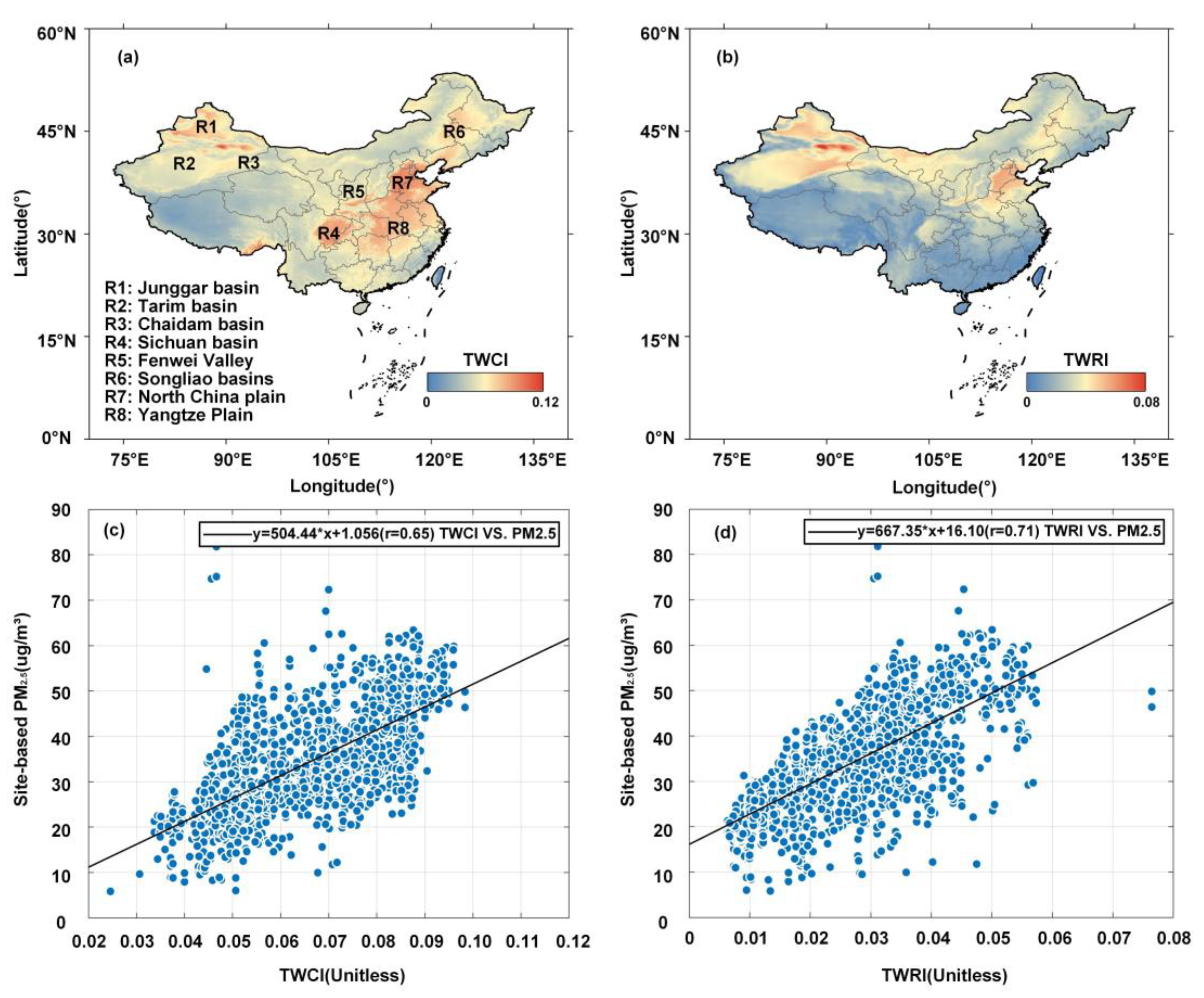
Beyond window selection, Figure 4 compares the spatial distribution of annual TWCI and TWRI. Spatially, there are distinct differences between the two models. TWCI (Figure 4a) showed high-value areas concentrated in regions like the Junggar Basin, Sichuan Basin, Fen-Wei River Valley, Songliao Basin, and from North to Central China, extending to the Yangtze River Plain. In contrast, the TWRI (depicted in Figure 4b) displayed high-value regions predominantly in the North China Plain and the eastern Tarim Basin, with markedly lower values observed in Southern China. Relative to TWCI, the spatial distribution of TWRI distinctly delineates the differences between China’s northern and southern regions.
Furthermore, the correlation between annual TWRI and site-based PM2.5 was compared, improving from the previous 0.65 to 0.71, showing a slight enhancement in correlation. Consequently, the TWRI model, which incorporates relative humidity, provided a more accurate simulation of the coupling effect of natural elements affecting PM2.5 concentrations compared to TWCI.

3.1.2. Comparison between Seasonal TWRI and TWCI

Figure 5 illustrates that the R value (correlation coefficients) between TWRI and PM2.5 across different seasons in China varied from 0.46 to 0.67, with specific values for spring, summer, autumn, and winter being 0.46, 0.66, 0.56, and 0.67, respectively. In contrast, the R values between TWCI and PM2.5 ranged from 0.41 to 0.67, with seasonal values of 0.41, 0.51, 0.54, and 0.67, respectively. TWRI significantly enhanced the correlation with PM2.5 concentration in summer, while other seasons showed slight improvements compared to TWCI. This may be due to the most significant deposition being caused by summer rainfall.
Figure 6 illustrates the quarterly changes in the spatial distribution of TWRI, TWCI, and PM2.5. TWRI maintained a relatively high value in closed areas within a year compared to TWCI, such as the Junggar basin (R1), Tarim basin (R2), Chaidam basin (R3), Sichuan (R4) basin, the Fenwei Valley (R5), Song Liao basins (R6) and the North China plain (R7). The difference is that the Yangtze Plain (R8) had a significant low value compared to TWCI.
Correspondingly, the quarterly spatial distributions of PM2.5 and TWCI are shown in Figure 6e–h,i–l. The seasonal temporal and spatial distributions of TWCI (Figure 6e–h) did not reflect the differences between humid and arid regions in China, resulting in almost identical TWCI values in the Sichuan Basin, North China plain, and Central China plain, an output which was significantly different from the seasonal spatio-temporal distribution of PM2.5. Taking the North China Plain in summer as an example, it exemplifies a typical semi-enclosed region where the Yanshan Mountains to the north and the Taihang Mountains to the west restrict the dispersion of air pollutants toward the west and the north, respectively. The dominant southerly winds, interacting with these mountain ranges, create a fully closed area that obstructs the horizontal diffusion of PM2.5. Additionally, the planetary boundary layer acts as a barrier to the vertical dispersion of pollutants, forming a closed three-dimensional space delineated by the TWCI. In the summer, however, the prevailing southerly winds contribute to significant rainfall in the area, promoting the deposition of pollutants and, thereby, reducing PM2.5 concentrations. This phenomenon is more pronounced in southern China and subtropical regions and is characterized by the TWRI.

3.2. PM2.5 Estimation

3.2.1. Descriptive Statistics

Table 2 summarizes the mean changes in the variables used in the PM2.5 prediction model for each season in China. The annual PM2.5 concentration in China was 38.68 ± 32.28 μ g / m 3 , with the highest concentration observed in winter at 58.27 ± 23.51 μ g / m 3 and the lowest observed in summer at 19.95 ± 7.86 μ g / m 3 . The annual average AOD in China was 0.22 ± 0.21, with little seasonal variation: the values from spring to winter were 0.12 ± 0.07, 0.04 ± 0.03, 0.08 ± 0.05, and 0.10 ± 0.16, respectively. The relative humidity was highest in summer, with a value of 73.67 ± 10.75%, while it attained its lowest in winter, with a value of 58.99 ± 15.36%. The boundary layer was at its lowest in winter, at 0.38 ± 0.10 km, while it was at its highest in the summer, at 1.16 ± 0.51 km. The highest wind speed was recorded in winter and reached 1.31 ± 0.74 m/s, while the lowest was recorded in autumn, reaching 0.77 ± 0.19 m/s. TWRI also varied, but the difference was not significant: from spring to winter, the values were 28.01 ± 12.07, 28.40 ± 13.08, 26.42 ± 11.65, and 28.87 ± 14.22, respectively. Most parameters almost reached their extreme values during summer and winter, a phenomenon which may be influenced by both meteorological factors and seasonal emission differences.
Table 3 details the correlations between various variables and PM2.5 concentrations at the monitoring stations. Research has shown that AOD has the highest correlation with PM2.5, followed by TWRI. In addition, the correlation between all variables and PM2.5 was almost at its weakest in spring, while it attained its highest in autumn or winter.

3.2.2. Model Fitting and Validation

The results of the fitting and validation are illustrated in Table 4 for three models in 2020 for China. It is observed that the fitting and validation accuracies of the three models were not significantly different, indicating that the model fitting effect was valid and there was no overfitting phenomenon. The optimized model had the best fitting effect for the entire year, with R2 values > 0.8, and RMSE and MAE values of < 10 μ g / m 3 and 7 μ g / m 3 , respectively. The coupled model had the lowest fitting effect, with R2 values of 0.68, 0.70, 0.75, and 0.74 for a year, while the R2 values of traditional models remained stable at 0.78.
Similarly, there was a similar trend in verifying accuracy. Among the three models, the optimized model had the highest R2 values of 0.76, 0.78, 0.79, and 0.82 for the four seasons, respectively. The coupled model had the lowest R2 values, which were 0.66, 0.68, 0.71, 0.73 for the four seasons, respectively. Although relatively low, such values are not far from traditional models, with values of 0.74, 0.74, 0.75, 0.76.
In addition, the coupled model and optimized model had the lowest R2 in spring (0.66, 0.76, respectively), and the highest in winter (0.73, 0.82, respectively), showing similar seasonal characteristics. This is related to the poor ability of TWRI to capture particulate matter concentration in spring and its better ability to capture particulate matter concentrations in winter. Furthermore, summer had the lowest RMSE and MAE values, while winter had the highest RMSE and MAE estimates among all models, a phenomenon which is related to increased anthropogenic emissions during winter and rainfall during summer [38].
Figure 7 illustrates the density scatterplots of the validation results for the traditional model, the coupled model, and the optimized model. There was no significant difference in the distribution of predicted and observed values in the four seasons among the three models, and there was an underestimation phenomenon in all models, with slopes < 0.85. The scatter points of the optimized model were more concentrated, while the scatter points of the coupled model were more scattered, a phenomenon which is related to its R2.

3.2.3. PM2.5 Spatial Distribution

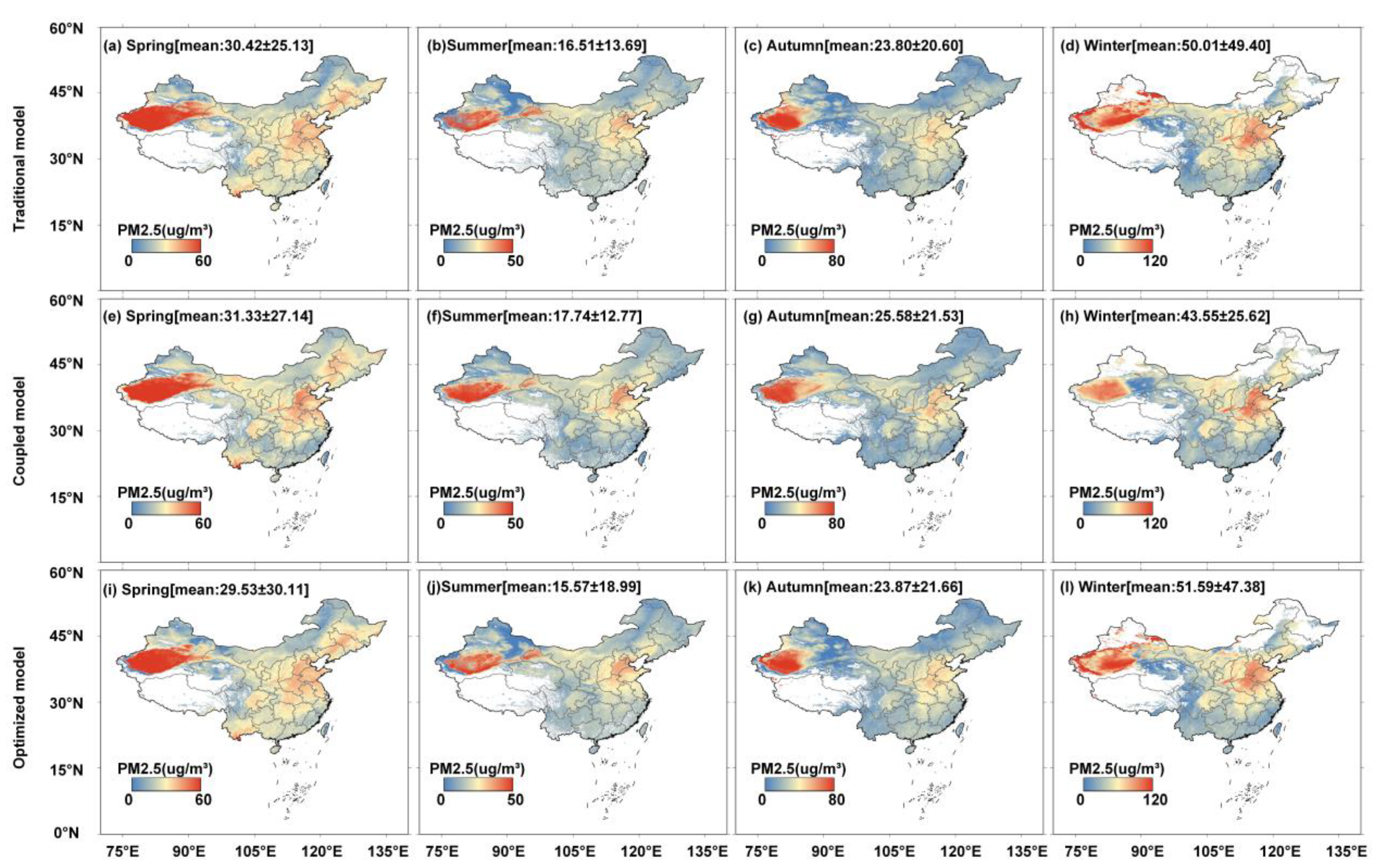
Figure 8 illustrates the quarterly PM2.5 spatial distribution across China from three models in 2020. On the seasonal scale, data are missing in southern China and northeastern and northwestern China because of the cloud cover in summer and the snow cover in winter. In terms of overall spatial distribution, all three models share the same characteristics in terms of seasonal variation. Significant areas of high concentration were identified in the Tarim Basin and the North China Plain, whereas significantly low concentration areas were observed in northeastern and southern China. Additionally, seasonal variations revealed significant spatial differences in fine particulate pollution. Winter experienced the most severe air pollution (50.01 ± 49.49, 43.55 ± 25.62, 51.59 ± 47.38 μ g / m 3 ), while summer experienced the lowest level of air pollution (16.51 ± 13.69, 17.74 ± 12.77, 15.57 ± 18.99 μ g / m 3 ). On the one hand, the seasonal fluctuations in PM2.5 levels can be attributed to lower emissions in summer and higher emissions in winter due to heating requirements. On the other hand, the summer monsoon contributes to increased rainfall that helps mitigate pollution levels, whereas in winter lower wind speeds and shallower boundary layers hinder the dispersion of pollutants. Moreover, PM2.5 concentrations tend to be less pronounced during the spring and autumn seasons.
Additionally, the inversion results from the coupled model were more centralized, mainly evidenced by the high concentration values that were concentrated in closed areas such as basins and valleys, in stark contrast with the surrounding results. The traditional model produced a more averaged distribution, with indistinct boundaries of high concentration and no significant differences between the central and southern regions. The optimized model merged the advantages of both, offering more distinct boundaries for high concentration areas while also providing relatively lower predicted results in the southern regions.

3.2.4. Regional PM2.5

The North China Plain, the Yangtze River Delta region, and the Pearl River Delta region were selected as heavily polluted areas for regional analysis. Quarterly performance of three models in these regions was evaluated to assess their effectiveness in capturing variations in pollution levels.
(1)
North China Plain
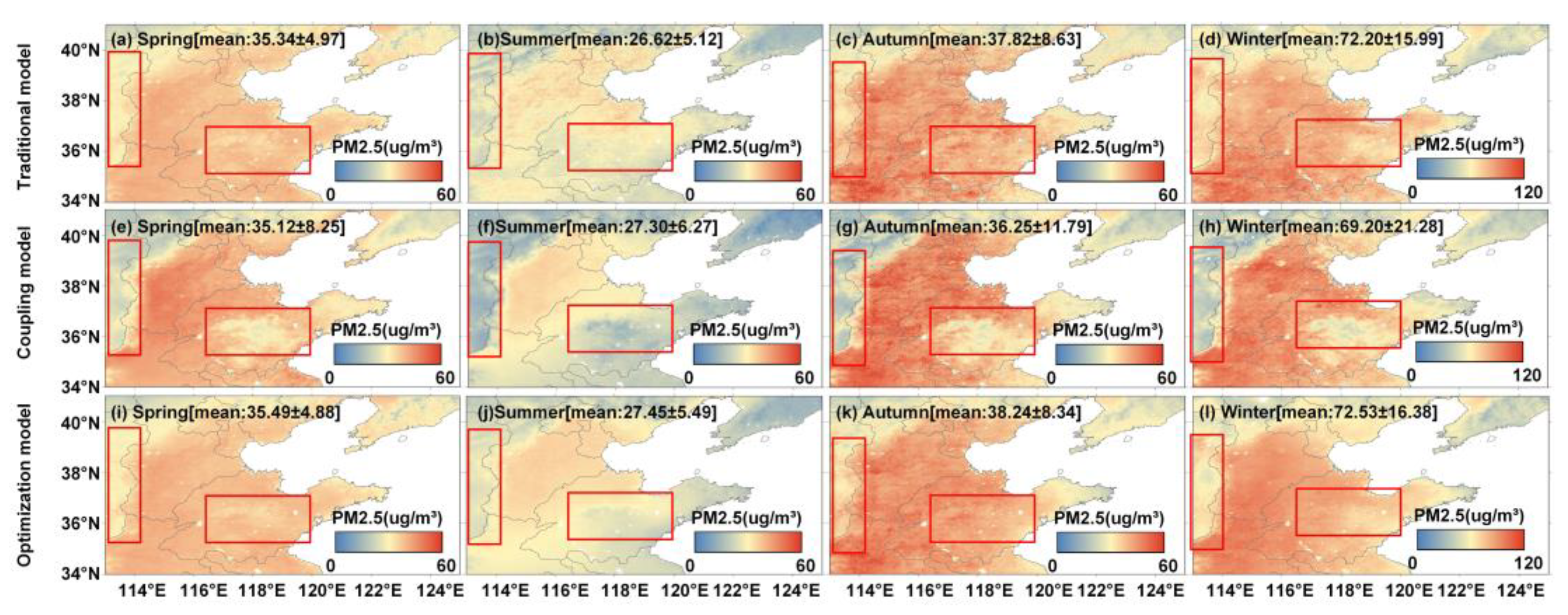
A comparison of three different models for the seasonal variation in PM2.5 over the North China Plain is shown in Figure 9. Consistent with previous studies, the models indicated lower concentrations during summer, higher in winter, and comparable levels in spring and autumn. The coupled model consistently exhibited the lowest mean concentrations across all seasons, but also the highest standard deviation. This suggests that the inverted results from the coupled model featured a broad distribution, highlighting the disparities between high and low concentrations, particularly between the Taihang Mountains and the North China Plain (highlighted by the red line frame on the left side of Figure 9). Furthermore, in comparison with the traditional model, the coupled model captured lower values in the Taishan Mountain range (Figure 9e,g, highlighted by the red line frame on the right side). The optimized model bore more resemblance to the traditional model, yet it captured variations in the Taishan Mountains (Figure 9 i,k,l), though these were not significant. In addition, its measurements were marginally lower in the Taihang and Yanshan Mountains, with more distinct differences observed between the mountains and the plains.
Table 5 shows the accuracy verification results associated with stations located in the North China Plain. Overall, among the three models, the optimized model had the highest inversion accuracy, followed by the traditional model and the coupled model, which had the lowest inversion accuracy. In terms of quarterly changes, the three models achieved the highest accuracy in autumn with R2 values of 0.72, 0.64, and 0.79, respectively, while the lowest occurred in summer with R2 values of 0.49, 0.42, and 0.60, respectively.
(2)
Pearl River Delta
As shown in Figure 10, the concentration of PM2.5 in the Pearl River Delta varied seasonally. There was, typically, a decrease in PM2.5 levels during the summer and an increase in PM2.5 levels during the winter, with minimal variation during spring and autumn. Since seasonal emissions showed minimal variation, this is primarily influenced by meteorological factors. The summer monsoon, bringing rainfall, leads to pollutant deposition and reduced PM2.5 concentrations. Conversely, during winter, weaker winds and a lower planetary boundary layer promote particle accumulation. Among the three models, the coupled model consistently exhibited lower average concentrations throughout the year. In comparison with the traditional model, both the coupled and optimized models emphasized areas of high concentration surrounding Guangzhou (Figure 10e–l, marked by a red wireframe). The coupled and optimized models also showed lower values in the northern mountainous regions of the Pearl River Delta compared with the traditional model (Figure 10d,h,l).
Table 6 shows the accuracy verification results associated with stations located in the Pearl River Delta. Similarly to the North China Plain, the optimized model had the highest inversion accuracy, followed by the traditional model and the coupled model, which had the lowest inversion accuracy. However, there was no significant indication of change regarding the seasonal variations. In the traditional model, the accuracy was highest in summer and lowest in autumn, with values of 0.5901 and 0.3351, respectively. In the coupled model, the accuracy was highest in spring and lowest in autumn, with values of 0.2936 and 0.1782, respectively. In the optimized model, the accuracy was highest in summer and lowest in winter, with values of 0.6287 and 0.4363, respectively.
(3)
Yangtze River Delta
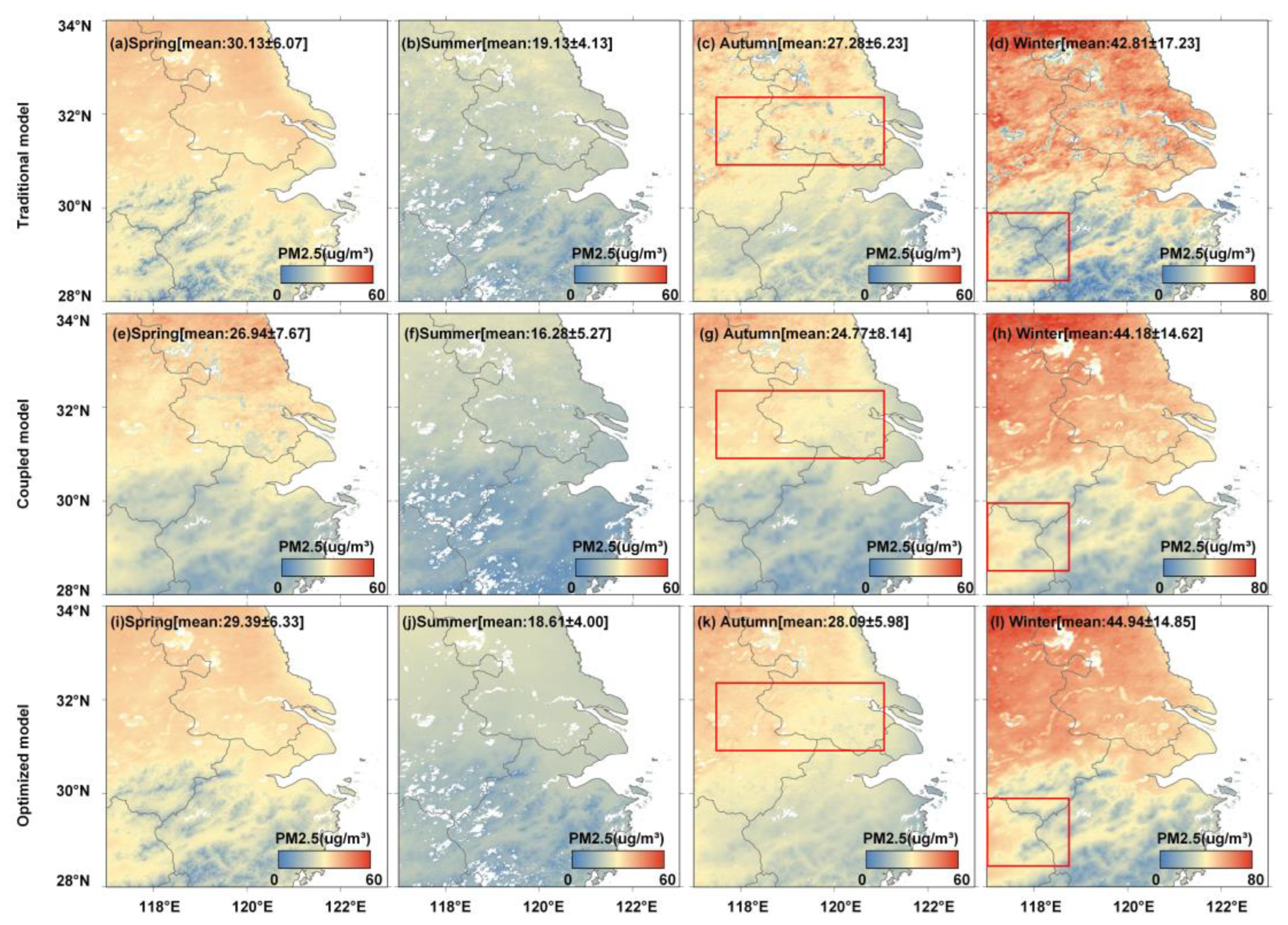
Figure 11 illustrates the PM2.5 concentrations across the Yangtze River Delta. Consistent with the two other areas, the concentration of PM2.5 in this region also varied seasonally—low values in summer, high values in winter, and minimal differences between spring and autumn. There were significant north–south disparities in PM2.5 levels, with higher concentrations observed in the north and lower concentrations observed in the south. This pattern largely stems from the northern area location on the Jianghuai Plain, where a dense population and industrial activities contribute to greater emissions, unlike the less populated hilly and mountainous terrain in the south which generates fewer emissions. Of the three models analyzed, the coupled model consistently exhibited the lowest average inversion values on a seasonal scale, while the optimized model exhibited the highest average. Spatially, however, no significant differences were evident among the models in this region.
Table 7 shows the accuracy verification results associated with stations located in the Yangtze River Delta. Similarly to the first two regions, the optimized model still achieved the highest accuracy among the three models. However, in this region, the coupled model exhibited slightly higher accuracy values than the traditional model in autumn and winter, and lower in spring and summer. In terms of quarterly changes, the three models achieved the highest accuracy in winter with R2 values of 0.5852, 0.7595, and 0.7713, respectively, while the lowest occurred in summer with R2 values of 0.2722, 0.2011, and 0.3292, respectively.

3.3. Discussion

Considering the impact of rainfall deposition on particulate matter, along with relative humidity and TWCI, the TWRI model was proposed. Compared to the TWCI model, TWRI exhibited enhanced stability and robustness, particularly manifesting increased boundary effects in closed areas, especially during summer and in South China. This suggests that TWRI more effectively captured the restrictive impact of topographical and meteorological factors on PM2.5 concentrations, primarily attributed to the predominant deposition effects brought by summer rainfall in humid regions, such as Southern China.
Subsequently, we employed a geographically weighted regression to use TWRI as an index for seasonal inversion. We compared the fitting and verification accuracies of traditional, coupled, and optimized models. The results revealed that: (1) using TWRI alone resulted in a slight decrease in accuracy compared to traditional models, yet the difference was minimal. Integrating the TWRI factor, however, led to improved accuracy. (2) There was little difference in fitting accuracy across seasons in the traditional model, but the lowest fitting accuracy was observed in spring, and the highest in winter within the coupled and optimized models incorporating the TWRI factor. This can be attributed to the fact that (a) TWRI represents a coupling effect of natural factors which does not encompass all mechanisms, thus solely using TWRI and AOD for inversion led to decreased accuracy; (b) in the optimized model, all natural factors were included, reflecting their individual impacts considered in traditional models, although the coupling effect represented by TWRI was not considered, hence its inclusion improved the accuracy; lastly, (c) the differential seasonal fitting performance, with spring being the worst and winter the best, also influenced the inversion accuracy, resulting in poorer performance in spring and enhanced performance in winter.
The spatial distribution of inversion results was analyzed across the different seasons on mainland China using the three models, with a particular emphasis on hotspot regions including the North China Plain, the Pearl River Delta, and the Yangtze River Delta. The results show that using TWRI alone resulted in higher concentration values being more concentrated in closed areas, with clearer boundaries between high- and low-value areas. This primarily stems from the fact that traditional models consider only the magnitude of meteorological and topographical factors, without accounting for the combined effects of these factors on closed areas, where the boundaries of these coupling effects are more distinct.
Furthermore, a comparative analysis of site-specific inversion accuracies revealed that, generally, the accuracies of all models were lower at the local level than at the national level, likely due to the utilization of nationwide data for model fitting. Additionally, within the three studied regions, the optimized model consistently demonstrated the highest inversion accuracy, followed by the traditional model, with the coupled model exhibiting the lowest accuracy. Notably, the coupled model integrating the TWRI achieved its highest accuracy in the North China Plain, with decreased accuracy in the Yangtze River Delta and the lowest accuracy in the Pearl River Delta. This variation can be attributed to the more pronounced coupled meteorological characteristics (closed effect) represented by TWRI in the North China Plain, as opposed to the weaker effects in the Yangtze and Pearl River Deltas. These findings suggest that inversion models incorporating TWRI are particularly effective in areas characterized by significant closed effects, such as basins and valleys, whereas their performance may be less pronounced in plains and mountainous regions.
However, some limitations/errors remain in this study. First, the TWRI model primarily uses relative humidity to represent changes in rainfall, overlooking the hygroscopic growth effect of relative humidity. Secondly, owing to a lack of daily TWRI data, seasonal averages were used in model fitting and validation, resulting in an insufficient number of sample points.

4. Conclusions

In this article, we introduce the TWRI model to represent the coupling effects of meteorological and topographical factors on PM2.5 concentrations and utilize this index to estimate seasonal surface PM2.5 concentrations. Compared to the TWCI model, TWRI more accurately simulates the spatial distribution and seasonal variations of particulate matter concentrations. By incorporating TWRI into PM2.5 inversions, seasonal accuracy improved by 1.3%, 5.4%, 4%, and 7.9% compared to the traditional model. Furthermore, inversions using TWRI more effectively delineate the boundaries and disparities between high and low concentration areas, especially in humid regions like South China. TWRI introduces a novel parameter in the PM2.5 inversion process, enhancing estimation accuracy and improving the fidelity of spatial distributions. It offers new insights into the coupling effects of natural meteorological elements on particulate matter and provides fresh perspectives for PM2.5–AOD inversion studies.
Future research should focus on developing coupled models that consider hygroscopic growth effects and on creating daily TWRI to enable PM2.5 inversions based on daily data.

Author Contributions

L.W. initiated and supervised this research. B.P. conducted the modeling and analysis and drafted the manuscript guided by L.W. and W.W. B.X. developed the original TWCI model guided by L.W. and W.W. and provided support for the development of the presented TWRI model. All authors have read and agreed to the published version of the manuscript.

Funding

This study was jointly supported by the Basic Science-Center Project of National Natural Science Foundation of China (72088101), the National Key Research and Development Program of China under Grant (2023YFE0208000), and the National Natural Science Foundation of China (42371392).

Data Availability Statement

The original contributions presented in the study are included in the article, further inquiries can be directed to the corresponding author.

Acknowledgments

The authors are grateful to CNEMC, ERA, the data center of NASA, and USGS for providing the datasets used in this study.

Conflicts of Interest

The authors declare no conflict of interest.

References

  1. Yin, P.; Brauer, M.; Cohen, A.J.; Wang, H.D.; Li, J.; Burnett, R.T.; Stanaway, J.D.; Causey, K.; Larson, S.; Godwin, W.; et al. The effect of air pollution on deaths, disease burden, and life expectancy across China and its provinces, 1990-2017: An analysis for the Global Burden of Disease Study 2017. Lancet Planet. Health 2020, 4, E386–E398. [Google Scholar] [CrossRef] [PubMed]
  2. Steffen, W.; Richardson, K.; Rockström, J.; Cornell, S.E.; Fetzer, I.; Bennett, E.M.; Biggs, R.; Carpenter, S.R.; de Vries, W.; de Wit, C.A.; et al. Planetary boundaries: Guiding human development on a changing planet. Science 2015, 347, 1259855. [Google Scholar] [CrossRef] [PubMed]
  3. Cohen, A.J.; Brauer, M.; Burnett, R.; Anderson, H.R.; Frostad, J.; Estep, K.; Balakrishnan, K.; Brunekreef, B.; Dandona, L.; Dandona, R.; et al. Estimates and 25-year trends of the global burden of disease attributable to ambient air pollution: An analysis of data from the Global Burden of Diseases Study 2015. Lancet 2017, 389, 1907–1918. [Google Scholar] [CrossRef] [PubMed]
  4. Dominici, F.; Peng, R.D.; Bell, M.L.; Pham, L.; McDermott, A.; Zeger, S.L.; Samet, J.M. Fine particulate air pollution and hospital admission for cardiovascular and respiratory diseases. JAMA-J. Am. Med. Assoc. 2006, 295, 1127–1134. [CrossRef]
  5. Liu, C.; Hu, H.; Zhou, S.; Chen, X.L.; Hu, Y.T.; Hu, J.L. Change of Composition, Source Contribution, and Oxidative Effects of Environmental PM2.5 in the Respiratory Tract. Environ. Sci. Technol. 2023, 57, 11605–11611. [Google Scholar] [CrossRef] [PubMed]
  6. Shu, Z.; Zhao, T.; Liu, Y.; Zhang, L.; Ma, X.; Kuang, X.; Li, Y.; Huo, Z.; Ding, Q.; Sun, X.; et al. Impact of deep basin terrain on PM(2.5) distribution and its seasonality over the Sichuan Basin, Southwest China. Environ. Pollut. 2022, 300, 118944. [Google Scholar] [CrossRef] [PubMed]
  7. Qi, L.; Zheng, H.; Ding, D.; Ye, D.; Wang, S. Effects of Meteorology Changes on Inter-Annual Variations of Aerosol Optical Depth and Surface PM2.5 in China—Implications for PM2.5 Remote Sensing. Remote Sens. 2022, 14, 2762. [Google Scholar] [CrossRef]
  8. Zhai, S.X.; Jacob, D.J.; Wang, X.; Shen, L.; Li, K.; Zhang, Y.Z.; Gui, K.; Zhao, T.L.; Liao, H. Fine particulate matter (PM2.5) trends in China, 2013–2018: Separating contributions from anthropogenic emissions and meteorology. Atmos. Chem. Phys. 2019, 19, 11031–11041. [Google Scholar] [CrossRef]
  9. Lelieveld, J.; Evans, J.S.; Fnais, M.; Giannadaki, D.; Pozzer, A. The contribution of outdoor air pollution sources to premature mortality on a global scale. Nature 2015, 525, 367–371. [Google Scholar] [CrossRef] [PubMed]
  10. Ding, Y.T.; Zhang, M.; Qian, X.Y.; Li, C.R.; Chen, S.; Wang, W.W. Using the geographical detector technique to explore the impact of socioeconomic factors on PM2.5 concentrations in China. J. Clean. Prod. 2019, 211, 1480–1490. [Google Scholar] [CrossRef]
  11. Liu, B.; Ma, X.; Ma, Y.; Li, H.; Jin, S.; Fan, R.; Gong, W. The relationship between atmospheric boundary layer and temperature inversion layer and their aerosol capture capabilities. Atmos. Res. 2022, 271, 106121. [Google Scholar] [CrossRef]
  12. Chen, X.; Ye, J. When the wind blows: Spatial spillover effects of urban air pollution in China. J. Environ. Plan. Manag. 2018, 62, 1359–1376. [Google Scholar] [CrossRef]
  13. Liu, B.Y.; Wang, L.L.; Zhang, L.; Bai, K.X.; Chen, X.F.; Zhao, G.N.; Yin, H.T.; Chen, N.; Li, R.; Xin, J.Y.; et al. Evaluating urban and nonurban PM2.5 variability under clean air actions in China during 2010-2022 based on a new high-quality dataset. Int. J. Digit. Earth 2024, 17, 2310734. [Google Scholar] [CrossRef]
  14. Zhang, Q.; Zheng, Y.X.; Tong, D.; Shao, M.; Wang, S.X.; Zhang, Y.H.; Xu, X.D.; Wang, J.N.; He, H.; Liu, W.Q.; et al. Drivers of improved PM2.5 air quality in China from 2013 to 2017. Proc. Natl. Acad. Sci. USA 2019, 116, 24463–24469. [Google Scholar] [CrossRef] [PubMed]
  15. Zhang, Y.-L.; Cao, F. Fine particulate matter (PM2.5) in China at a city level. Sci. Rep. 2015, 5, 14884. [Google Scholar] [CrossRef] [PubMed]
  16. Yang, Z.M.; Zdanski, C.; Farkas, D.; Bang, J.; Williams, H. Evaluation of Aerosol Optical Depth (AOD) and PM2.5 associations for air quality assessment. Remote Sens. Appl.-Soc. Environ. 2020, 20, 100396. [Google Scholar] [CrossRef]
  17. Yang, Q.; Yuan, Q.; Yue, L.; Li, T.; Shen, H.; Zhang, L. The relationships between PM2.5 and aerosol optical depth (AOD) in mainland China: About and behind the spatio-temporal variations. Environ. Pollut. 2019, 248, 526–535. [Google Scholar] [CrossRef] [PubMed]
  18. Xu, W.; Wang, W.; Wang, N.; Chen, B. A New Algorithm for Himawari-8 Aerosol Optical Depth Retrieval by Integrating Regional PM₂.₅ Concentrations. IEEE Trans. Geosci. Remote Sens. 2022, 60, 4106711. [Google Scholar] [CrossRef]
  19. Yang, Q.; Yuan, Q.; Yue, L.; Li, T. Investigation of the spatially varying relationships of PM2.5 with meteorology, topography, and emissions over China in 2015 by using modified geographically weighted regression. Environ. Pollut. 2020, 262, 114257. [Google Scholar] [CrossRef] [PubMed]
  20. Hammer, M.S.; van Donkelaar, A.; Li, C.; Lyapustin, A.; Sayer, A.M.; Hsu, N.C.; Levy, R.C.; Garay, M.J.; Kalashnikova, O.V.; Kahn, R.A.; et al. Global Estimates and Long-Term Trends of Fine Particulate Matter Concentrations (1998–2018). Environ. Sci. Technol. 2020, 54, 7879–7890. [Google Scholar] [CrossRef] [PubMed]
  21. Zhu, S.T.; Tang, J.Y.; Zhou, X.L.; Li, P.; Liu, Z.L.; Zhang, C.C.; Zou, Z.Y.; Li, T.; Peng, C.H. Research progress, challenges, and prospects of PM2.5 concentration estimation using satellite data. Environ. Rev. 2023, 31, 605–631. [Google Scholar] [CrossRef]
  22. Wang, W.; Mao, F.; Du, L.; Pan, Z.; Gong, W.; Fang, S. Deriving Hourly PM2.5 Concentrations from Himawari-8 AODs over Beijing–Tianjin–Hebei in China. Remote Sens. 2017, 9, 858. [Google Scholar] [CrossRef]
  23. Bai, Y.; Wu, L.; Qin, K.; Zhang, Y.; Shen, Y.; Zhou, Y. A Geographically and Temporally Weighted Regression Model for Ground-Level PM2.5 Estimation from Satellite-Derived 500 m Resolution AOD. Remote Sens. 2016, 8, 262. [Google Scholar] [CrossRef]
  24. He, Q.; Huang, B. Satellite-based mapping of daily high-resolution ground PM2.5 in China via space-time regression modeling. Remote Sens. Environ. 2018, 206, 72–83. [Google Scholar] [CrossRef]
  25. Song, S.; Gao, M.; Xu, W.; Sun, Y.; Worsnop, D.R.; Jayne, J.T.; Zhang, Y.; Zhu, L.; Li, M.; Zhou, Z.; et al. Possible heterogeneous chemistry of hydroxymethanesulfonate (HMS) in northern China winter haze. Atmos. Chem. Phys. 2019, 19, 1357–1371. [Google Scholar] [CrossRef]
  26. Ning, G.; Wang, S.; Ma, M.; Ni, C.; Shang, Z.; Wang, J.; Li, J. Characteristics of air pollution in different zones of Sichuan Basin, China. Sci. Total Environ. 2018, 612, 975–984. [Google Scholar] [CrossRef] [PubMed]
  27. Karle, N.N. Studies of the Planetary Boundary Layer and their Impact on Air Pollution in a Semi-Arid Region with Complex Terrain; The Unisversity of Texas: El Paso, TX, USA, 2021. [Google Scholar]
  28. Tang, Y.; Xie, S.; Huang, L.; Liu, L.; Wei, P.; Zhang, Y.; Meng, C. Spatial Estimation of Regional PM2.5 Concentrations with GWR Models Using PCA and RBF Interpolation Optimization. Remote Sens. 2022, 14, 5626. [Google Scholar] [CrossRef]
  29. Ding, W.; Zhu, Y. Prediction of PM2.5 Concentration in Ningxia Hui Autonomous Region Based on PCA-Attention-LSTM. Atmosphere 2022, 13, 1444. [Google Scholar] [CrossRef]
  30. Zhang, T.; Zang, L.; Wan, Y.; Wang, W.; Zhang, Y. Ground-level PM2.5 estimation over urban agglomerations in China with high spatiotemporal resolution based on Himawari-8. Sci. Total Environ. 2019, 676, 535–544. [Google Scholar] [CrossRef] [PubMed]
  31. Wu, L.; Xie, B.; Wang, W. Quantifying the impact of terrain–wind–governed close-effect on atmospheric polluted concentrations. J. Clean. Prod. 2022, 367, 132995. [Google Scholar] [CrossRef]
  32. Lyapustin, A.; Wang, Y. MCD19A2 MODIS/Terra+Aqua Land Aerosol Optical Depth Daily L2G Global 1 km SIN Grid V006. [Dataset], NASA EOSDIS Land Processes DAAC, 2018. Available online: https://lpdaac.usgs.gov/products/mcd19a2v006/ (accessed on 9 June 2024).
  33. Urraca, R.; Huld, T.; Gracia-Amillo, A.; Martinez-de-Pison, F.J.; Kaspar, F.; Sanz-Garcia, A. Evaluation of global horizontal irradiance estimates from ERA5 and COSMO-REA6 reanalyses using ground and satellite-based data. Sol. Energy 2018, 164, 339–354. [Google Scholar] [CrossRef]
  34. Schnell, J.L.; Naik, V.; Horowitz, L.W.; Paulot, F.; Mao, J.; Ginoux, P.; Zhao, M.; Ram, K. Exploring the relationship between surface PM2.5 and meteorology in Northern India. Atmos. Chem. Phys. 2018, 18, 10157–10175. [Google Scholar] [CrossRef]
  35. Liu, S.; Xing, J.; Sahu, S.K.; Liu, X.; Liu, S.; Jiang, Y.; Zhang, H.; Li, S.; Ding, D.; Chang, X. Wind-blown dust and its impacts on particulate matter pollution in Northern China: Current and future scenarios. Environ. Res. Lett. 2021, 16, 114041. [Google Scholar] [CrossRef]
  36. Zhang, L.; Guo, X.; Zhao, T.; Gong, S.; Xu, X.; Li, Y.; Luo, L.; Gui, K.; Wang, H.; Zheng, Y.; et al. A modelling study of the terrain effects on haze pollution in the Sichuan Basin. Atmos. Environ. 2019, 196, 77–85. [Google Scholar] [CrossRef]
  37. Oshan, T.M.; Smith, J.P.; Fotheringham, A.S. Targeting the spatial context of obesity determinants via multiscale geographically weighted regression. Int. J. Health Geogr. 2020, 19, 11. [Google Scholar] [CrossRef]
  38. Wei, J.; Huang, W.; Li, Z.; Xue, W.; Peng, Y.; Sun, L.; Cribb, M. Estimating 1-km-resolution PM2.5 concentrations across China using the space-time random forest approach. Remote Sens. Environ. 2019, 231, 111221. [Google Scholar] [CrossRef]
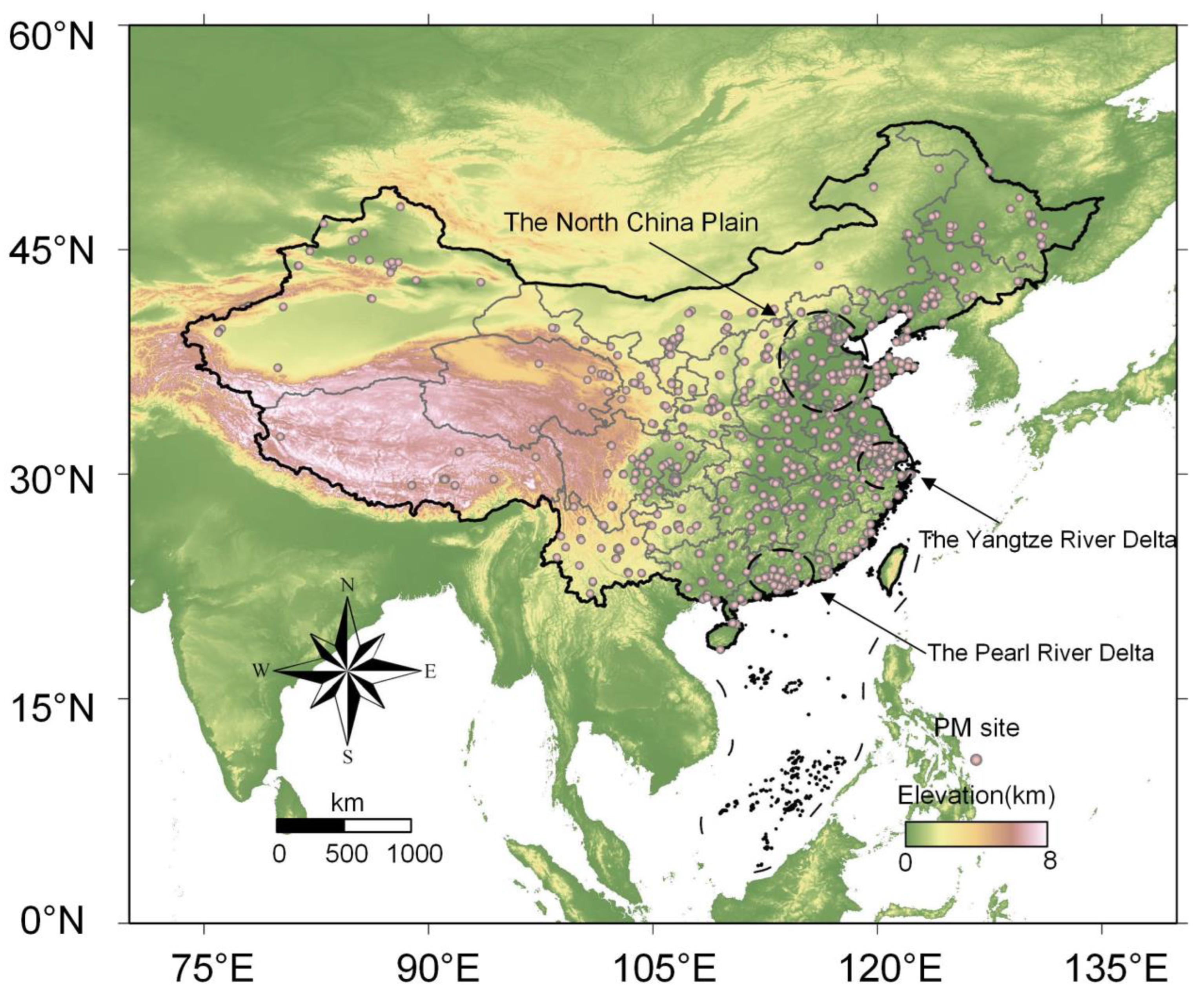
Figure 1. Spatial distribution of the study area and PM monitoring network in China.
Remotesensing 16 02145 g001
Figure 2. The overall workflow for this study.
Remotesensing 16 02145 g002
Figure 3. The correlation coefficient (R) between quarterly TWRI (a) and TWCI (b) with PM2.5 at stations vary with different window sizes.
Remotesensing 16 02145 g003
Figure 4. Spatial distributions of annual TWCI (a) and TWRI (b). Scatterplots of annual TWCI (c) and TWRI (d) with site-based PM2.5.
Remotesensing 16 02145 g004
Figure 5. Scatter plot of seasonal TWRI (ad) and TWCI (eh) with PM2.5 concentration at different stations.
Remotesensing 16 02145 g005
Figure 6. Spatial distribution of seasonal (ad) TWRI, (eh) TWCI, and(il) PM2.5 concentration for spring (a,e,i), summer (b,f,j), autumn (c,g,k), and winter (d,h,l) in China.
Remotesensing 16 02145 g006
Figure 7. Density scatterplots of 10-CV results from the GWR with traditional, coupled, and optimized models for spring (a,e,i), summer (b,f,j), autumn (c,g,k), and winter (d,h,l) in China. The dashed line and the solid line represent the 1:1 line and the linear regression line, respectively.
Remotesensing 16 02145 g007
Figure 8. Seasonal mean distributions of PM2.5 concentrations of three models for spring (ai), summer (bj), autumn (ck), and winter (dl) in 2020 across China.
Remotesensing 16 02145 g008
Figure 9. Zoomed-in map of seasonal distribution of PM2.5 concentration in 2020 of three models in the North China Plain: Traditional model (ad), Coupling model (eh) and Optimization model (il). The red wireframe indicates areas with significant differences among the three models.
Remotesensing 16 02145 g009
Figure 10. Zoomed-in map of seasonal concentration of PM2.5 in 2020 for three models in the Pearl River Delta: Traditional model (ad), Coupling model (eh) and Optimization model (il). The red wireframe indicates areas with significant differences among the three models.
Remotesensing 16 02145 g010
Figure 11. Zoomed-in map of the seasonal concentration of PM2.5 in 2020 for three models in the Yangtze River Delta region: Traditional model (ad), Coupling model (eh) and Optimization model (il). The red wireframe indicates areas with significant differences among the three models.
Remotesensing 16 02145 g011
Table 1. The main information of the obtained parameters in this study.
Variable NameSource Spatial Resolution Temporal Resolution Unit
Wind speedERA50.25° × 0.25°1 monthm/s
Wind directionERA50.25° × 0.25°1 month°
Boundary layer heightERA50.25° × 0.25°1 monthm
Relative humidityERA50.25° × 0.25°1 month%
DEMUSGS90 m-m
MODIS-AODMODIS0.01° × 0.01°1 day-
Ground-level PM2.5CNEMC-1 hμg/m3
Grid-level PM2.5WUSTL0.01° × 0.01°1 monthμg/m3
Table 2. Descriptive statistics of all variables for each season in China.
Season PM2.5 (μg/m3)AODRH (%)PBLH (km)WS (m/s)TWRI × 1000DEM (m)
SpringMin7.18020.250.220.166.270
N = 1484Max187.280.3785.721.423.4074.984101
Mean55.270.1258.990.580.9728.01426
Std.23.510.0715.360.160.5212.07725
SummerMin4.00022.170.210.175.46-
N = 1486Max83.350.2790.501.164.3469.73-
Mean19.950.0473.670.511.1728.40-
Std.7.860.0310.750.130.6213.08-
AutumnMin5.40027.340.170.226.53-
N = 1481Max82.920.2487.280.905.7282.54-
Mean31.390.0866.340.441.3026.42-
Std.11.150.0510.630.090.7711.65-
WinterMin7.18017.670.070.196.38-
N = 1447Max187.280.2787.091.285.1694.18-
Mean55.270.1064.690.381.3128.87-
Std.23.510.0610.970.100.7414.22-
Table 3. The correlation coefficient (R) between PM2.5 concentration and all variables in each season in China.
Season/RAODRH (%)PBLH (km)WS (m/s)TWRIDEM
Spring0.5888−0.29750.1129−0.25020.4603−0.2553
Summer0.7258−0.29170.0201−0.32960.6577−0.2123
Autumn0.7540−0.4059−0.3159−0.41380.5667−0.2829
winter0.5684−0.3480−0.4571−0.50770.6950−0.2906
Table 4. Model fitting and sample cross-validation results under different parameter combinations.
ModelModel FittingModel Validation
SpringSummerAutumnWinterSpringSummerAutumnWinter
GWR
(traditional model)
R2 = 0.78R2 = 0.77R2 = 0.78R2 = 0.78R2 = 0.75R2 = 0.74R2 = 0.76R2 = 0.76
RMSE = 4.71RMSE = 3.81RMSE = 5.24RMSE = 10.97RMSE = 5.04RMSE = 3.99RMSE = 5.51RMSE = 11.61
MAE = 3.57MAE = 2.90MAE = 3.95MAE = 7.95MAE = 3.78MAE = 3.04MAE = 4.16MAE = 8.35
GWR
(coupled model)
R2 = 0.68R2 = 0.70R2 = 0.72R2 = 0.74R2 = 0.66R2 = 0.68R2 = 0.71R2 = 0.73
RMSE = 5.95RMSE = 4.57RMSE = 6.16RMSE = 11.99RMSE = 6.13RMSE = 4.67RMSE = 6.30RMSE = 12.40
MAE = 4.53MAE = 3.55MAE = 4.74MAE = 8.47MAE = 4.66MAE = 3.63MAE = 4.84MAE = 8.69
GWR
(optimized model)
R2 = 0.80R2 = 0.80R2 = 0.82R2 = 0.84R2 = 0.76R2 = 0.78R2 = 0.79R2 = 0.82
RMSE = 4.47RMSE = 3.52RMSE = 4.80RMSE = 9.52RMSE = 4.90RMSE = 3.73RMSE = 5.12RMSE = 10.12
MAE = 3.32MAE = 2.67MAE = 3.60MAE = 6.61MAE = 3.56MAE = 2.83MAE = 3.84MAE = 7.00
Table 5. Model sample cross-validation results under different parameter combinations in North China Plain.
ModelModel Validation
SpringSummerAutumnWinter
Traditional modelR2 = 0.6038R2 = 0.4951R2 = 0.7209R2 = 0.6391
MAE = 3.1961MAE = 4.2243MAE = 4.5146MAE = 9.2194
RMSE = 4.3009RMSE = 5.2480RMSE = 5.8526RMSE = 13.5801
Coupled modelR2 = 0.4812R2 = 0.4205R2 = 0.6480R2 = 0.5728
MAE = 4.3503MAE = 4.4136MAE = 5.4437MAE = 10.4857
RMSE = 5.4718RMSE = 5.5517RMSE = 6.8394RMSE = 15.031
Optimized modelR2 = 0.6459R2 = 0.6028R2 = 0.7932R2 = 0.7078
MAE = 3.0781MAE = 3.7031MAE = 3.9485MAE = 8.0193
RMSE = 4.1251RMSE = 4.5989RMSE = 5.0712RMSE = 12.231
Table 6. Model sample cross-validation results under different parameter combinations in the Pearl River Delta.
ModelModel Validation
SpringSummerAutumnWinter
Traditional modelR2 = 0.4199R2 = 0.5901R2 = 0.3351R2 = 0.3779
MAE = 2.7604MAE = 1.8302MAE = 2.6256MAE = 4.6836
RMSE = 3.3114RMSE = 2.3255RMSE = 3.1117RMSE = 6.1177
Coupled modelR2 = 0.2936R2 = 0.1852R2 = 0.1782R2 = 0.2816
MAE = 2.5943MAE = 2.6615MAE = 3.3697MAE = 3.3234
RMSE = 3.3598RMSE = 3.5591RMSE = 4.5965RMSE = 4.0667
Optimized modelR2 = 0.5299R2 = 0.6287R2 = 0.4757R2 = 0.4363
MAE = 1.8325MAE = 1.7368MAE = 2.0630MAE = 2.7679
RMSE = 2.3227RMSE = 2.2703RMSE = 2.7055RMSE = 3.4448
Table 7. Model sample cross-validation results under different parameter combinations in the Yangtze River Delta.
ModelModel Validation
SpringSummerAutumnWinter
Traditional modelR2 = 0.4622R2 = 0.2722R2 = 0.5203R2 = 0.5852
MAE = 3.4077MAE = 2.6890MAE = 3.7955MAE = 7.7003
RMSE = 4.4071RMSE = 3.3348RMSE = 5.1042RMSE = 9.6655
Coupled modelR2 = 0.4520R2 = 0.2011R2 = 0.5909R2 = 0.7595
MAE = 3.8866MAE = 3.5427MAE = 3.8037MAE = 5.3997
RMSE = 5.0530RMSE = 4.4939RMSE = 4.8866RMSE = 7.2528
Optimized modelR2 = 0.5317R2 = 0.3492R2 = 0.6337R2 = 0.7713
MAE = 3.1902MAE = 2.5069MAE = 3.3545MAE = 5.3192
RMSE = 4.1344RMSE = 3.1245RMSE = 4.3711RMSE = 7.1304
Disclaimer/Publisher’s Note: The statements, opinions and data contained in all publications are solely those of the individual author(s) and contributor(s) and not of MDPI and/or the editor(s). MDPI and/or the editor(s) disclaim responsibility for any injury to people or property resulting from any ideas, methods, instructions or products referred to in the content.