Reconstruction of High-Resolution 3D GPR Data from 2D Profiles: A Multiple-Point Statistical Approach

Abstract

Ground-penetrating radar (GPR) is a popular geophysical tool for mapping the underground. High-resolution 3D GPR data carry a large amount of information and can greatly help to interpret complex subsurface geometries. However, such data require a dense collection along closely spaced parallel survey lines, which is time consuming and costly. In many cases, for the sake of efficiency, a choice is made during 3D acquisitions to use a larger spacing between the profile lines, resulting in a dense measurement spacing along the lines but a much coarser one in the across-line direction. Simple interpolation methods are then commonly used to increase the sampling before interpretation, which can work well when the subsurface structures are already well sampled in the across-line direction but can distort such structures when this is not the case. In this work, we address the latter problem using a novel multiple-point geostatistical (MPS) simulation methodology. For a considered 3D GPR dataset with reduced sampling in the across-line direction, we attempt to reconstruct a more densely spaced, high-resolution dataset using a series of 2D conditional stochastic simulations in both the along-line and across-line directions. For these simulations, the existing profile data serve as training images from which complex spatial patterns are quantified and reproduced. To reduce discontinuities in the generated 3D spatial structures caused by independent 2D simulations, the target profile being simulated is chosen randomly, and simulations in the along-line and across-line directions are performed alternately. We show the successful application of our approach to 100 MHz synthetic and 200 MHz field GPR data under multiple decimation scenarios where survey lines are regularly deleted from a dense 3D reference dataset, and the corresponding reconstructions are compared with the original data.

1. Introduction

Ground-penetrating radar (GPR) has gained widespread recognition as a geophysical tool for capturing high-resolution images of the shallow subsurface [1,2]. Traditionally, GPR measurements are acquired at regular intervals along one or a limited number of profile lines, resulting in what are commonly referred to as “2D data”. While this approach may be sufficient for studying simple subsurface environments, it falls short when dealing with complex subsurface geometries. Consequently, there has been a growing demand for three-dimensional (3D) GPR data acquisitions in recent years. These acquisitions typically involve surveying along closely spaced parallel survey lines to gain a more comprehensive understanding of near-surface structures [3]. The utilization of 3D GPR data has become increasingly common for various applications, including archaeological site investigation (e.g., [4,5]), bedrock fracture mapping (e.g., [3,6]), glacier drainage network imaging (e.g., [7,8]), transportation infrastructure characterization (e.g., [9,10]), and animal burrow mapping (e.g., [11,12]).

To acquire what are known as “full-resolution” 3D GPR data, Grasmueck et al. (2005) [3] suggest that the spacing between individual GPR measurements should be no greater than one quarter of the dominant wavelength of the GPR pulse in the studied medium. This ensures that the moveout of diffraction events is properly sampled in the time–space domain. While such data are of extremely high quality and permit high-resolution detailed images of subsurface structure in 3D (e.g., [6,13]), the required close line spacing makes it impractical in many cases to acquire them [14]. For 100 MHz center-frequency data in a soil having a radar velocity of 0.1 m/ns, for example, a sample spacing of 0.25 m is required for the full-resolution conditions to be satisfied. Considering a GPR line spacing equal to this value strongly limits the size of domain that can be surveyed. As a consequence, a typical trade-off in 3D data collection is that the line spacing is set to be significantly greater than the measurement spacing along the survey lines. This introduces a strong acquisition bias to the 3D dataset, which can adversely affect subsequent data processing steps such as migration [15], as well as data visualization and interpretation.

To address the aforementioned challenge, a common strategy in 3D GPR data processing is to use rudimentary interpolation methods to fill the gaps between existing parallel survey lines. This is typically done in two dimensions along horizontal “time slices” through the data, but may also be applied across profiles in the time–space domain. In this regard, a variety of interpolation methods have been considered, including linear (e.g., [16]), cubic spline (e.g., [17]), inverse distance weighting (e.g., [18]), and kriging interpolation (e.g., [19]). While the results of these methods vary and have been extensively investigated in past work (e.g., [20,21]), most methods perform reasonably well when the GPR line spacing is sufficiently dense to adequately sample the underlying reflection structures. However, in the presence of complex subsurface geometries and spatial aliasing in the across-line direction, both of which are common in 3D GPR datasets, these strategies become less effective. Indeed, as the line spacing increases, the quality of the reconstructed profiles obtained with simple interpolation methods degrades, leading to oversmoothed patterns that do not accurately represent the GPR reflection structures.

In the context of 3D archaeological investigations, Booth et al. (2008) [14] performed GPR data densification in the across-line direction using a 3D beam-steering technique, where the coherency of energy along specified dip trajectories was used to predict the GPR traces at the desired locations. Unlike the 2D interpolation methods described above, this approach effectively exploits the 3D nature of the data and can at least partly overcome the effects of aliasing. Other, more sophisticated methods for 3D interpolation have been developed in the reflection seismic industry to deal with aliased data. These methods typically take advantage of the predictability and/or sparseness of the data, commonly in a transformed domain, to estimate the missing traces (e.g., [15,22,23,24]). With all of such approaches, however, there exists the inherent assumption that the data exhibit a rather simple structure, typically meaning that they can be represented locally as a sum of linear “plane-wave” events. Unfortunately, such an assumption is overly restrictive for many 3D near-surface GPR datasets, where complex distributions of reflections and diffractions are common. Ideally, we seek a data densification methodology for GPR data that (i) takes into account the 3D nature of the measurements, (ii) avoids simplistic assumptions about the data structure, and (iii) can perform well in the presence of spatial aliasing.

Over the past two decades, multiple-point statistical (MPS) methods have gained popularity in the field of geostatistics due to their ability to capture and reproduce complex and realistic patterns [25]. Training images (TIs), which are assumed to share similar characteristics to the region of interest, provide spatial statistical relationships for the target variable(s), which are used alongside measured data to conditionally simulate stochastic realizations of the variable(s) at unknown locations. Recent research has shown the successful application of MPS methods to a wide variety of problems in the geosciences, including simulating complex geological structures (e.g., [26,27]), downscaling digital elevation models (e.g., [28,29]), gap filling incomplete satellite images (e.g., [30,31]), and generating rainfall time series (e.g., [32]). Most recently, MPS simulation was applied to the problem of reconstructing missing data along 2D GPR profiles [33]. Specifically, gap filling, trace-spacing regularization, and trace densification were all carried out using a single unified MPS approach with highly promising results. Given that 3D data reconstruction inherently presents greater challenges compared to 2D reconstruction, primarily due to increased computational demands, the lack of an adequate TI in 3D, and the need to ensure consistency in the simulated 3D structures, it is important to investigate the potential of MPS techniques for the 3D GPR data reconstruction problem.

In this paper, we build on the recent work of Zhang et al. (2024) [33] and investigate the potential of MPS methods for densifying 3D GPR data in the across-line direction, thereby addressing the acquisition bias problem mentioned above. Considering that a fully 3D TI is generally not available for such work, our research focuses on the use of 2D simulations in the along-line and across-line directions to reconstruct the 3D high-resolution GPR data volume from its low-resolution counterpart. The structure of this paper is as follows. First, we present a brief review of MPS methods and the MPS algorithm used in our research. Next, we describe the specific methodology that we employ for 3D GPR data reconstruction. Finally, we show and discuss the application of our methodology to synthetic and field datasets under multiple decimation scenarios, leading to a discussion of the results and future perspectives.

2. Methodology

2.1. Multiple-Point Statistical Simulation

Unlike traditional two-point geostatistical methods, MPS approaches examine relationships across numerous points in space, thereby enabling the reconstruction of highly complex and realistic patterns [25]. TIs, which are assumed to carry information compatible with the target area, are used to derive the higher-order spatial statistics required for simulation. The very first MPS simulation program for categorical (value-constrained) variables, named extended normal equation simulation (ENESIM), was developed by Guardiano and Srivastava (1993) [34]. With ENESIM, missing pixels (or voxels in 3D) are sequentially simulated by drawing from a conditional probability distribution that is determined by scanning the TI and counting the occurrences of patterns matching the surrounding informed points. Since ENESIM mandates a re-scan of the entire TI for each missing data point, it poses significant computational challenges. Strebelle (2002) [27] addressed this issue by scanning the TI only once and employing a hierarchical tree architecture to archive the complete TI statistics before the sequential simulation process. This led to the development of the simple normal equations simulation (SNESIM) program. However, the storage of such statistical data requires substantial memory, and the application of this approach was still limited to categorical variables [35]. Mariethoz et al. (2010) [36] pointed out that, in randomly searching a TI, matching patterns, or “data events”, should be found with a frequency according to their probability of occurrence. Based on this, the direct sampling (DS) technique was introduced, which bypasses the need to compute tables of statistics by directly extracting values from the TI as the matching patterns are identified. The latter approach significantly reduces storage demands and can be straightforwardly implemented in scenarios involving continuous variables as well as multivariate simulations.

2.2. Quick Sampling (QS) Algorithm

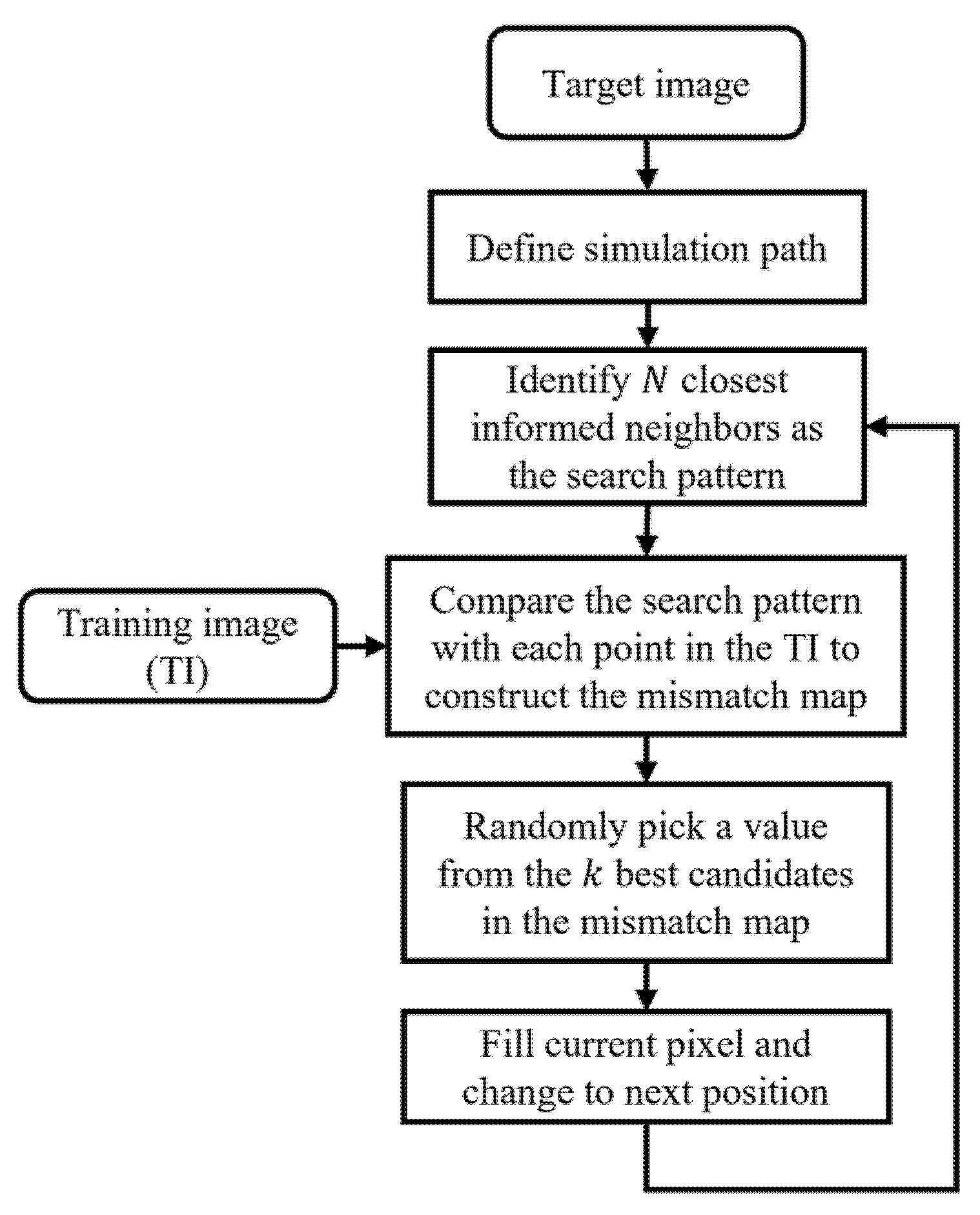
In this work, a highly efficient implementation of the DS approach called “quick sampling” (QS) [37] is considered for the MPS-based densification of 3D GPR data. The QS algorithm markedly speeds up the search process for identifying appropriate matches to the configuration of known or simulated data surrounding the point of interest through the use of cross-correlations that are carried out with the fast Fourier transform (FFT). Figure 1 presents a general workflow of the QS algorithm in the context of simulating missing pixels in a target image. First, a random simulation path is created through the target image along which the algorithm will visit all unknown pixels. For each pixel along this path, a search pattern or “data event” is defined based on the $N$ closest informed surrounding pixels, which comprise measured conditioning data and previously simulated values. Next, a “mismatch map” is created by calculating a pixel-wise dissimilarity metric between the search pattern and the TI at each spatial location. Using this map, the value simulated at the unknown pixel location is chosen at random from the $k$ best candidates having the smallest dissimilarity measure. The QS algorithm then proceeds to the next pixel and repeats this process until all unknown points along the simulation path have been populated. Note that, within the realm of GPR reconstruction, the term “pixel” refers to a GPR reflection amplitude value associated with a specific position along the Earth’s surface and two-way travel time.

Three parameters control the performance of the QS algorithm. The first is $N$, which is the number of closest informed pixels to consider around the unknown point. A higher $N$ value imposes more constraints around the missing point, leading to a better fit to the conditioning data. However, this carries the risk of introducing what is known as “verbatim copy” into the simulations, meaning that regions of the TI may be copied identically into the target image. A lower $N$ value, on the other hand, will avoid this issue but may result in a reduction in the realism of the simulated structures because not enough multi-point relationships are taken into account. The second QS parameter requiring definition is a weighting coefficient, $\alpha$, that determines the importance placed on closer pixels versus distant pixels in the dissimilarity calculation. A higher α value places greater weight on pixels nearest to the unknown point, which effectively limits the spatial extent of the data event and promotes a focus on local structures. In contrast, a lower α value places more weight on fitting distant pixels, which may improve the realism of the simulations but may also make it more challenging to find a suitable match. Finally, QS parameter $k$ controls the size of the candidate pool from which the simulated values are randomly drawn. Consistently selecting the positions in the TI corresponding to the lowest dissimilarity metric, meaning setting $k$ = 1, is not ideal because it poses the risk of verbatim copy. Conversely, having too large a candidate pool may result in the selection of inappropriate values and reduce the quality of the results. Note that, in practical applications of GPR data reconstruction using the QS algorithm, we have found that there is a relatively broad range of values for $N$, α, and $k$ that can yield high-quality simulation results [33]. Thus, although the choice of these parameters is important, it is rather straightforward and rapid to find acceptable values. For further details on the mathematical development of the QS algorithm along with a sensitivity analysis showing the effects of changing $N$, α, and $k$, we refer the reader to Gravey and Mariethoz (2020) [37]. For guidelines on the choice of $N$, α, and $k$ in the context of 2D GPR profile reconstruction, see Zhang et al. (2024) [33].

2.3. Application to 3D GPR Data Reconstruction

Although 3D MPS simulations with the QS approach are possible [37], two main challenges emerge when considering a 3D application of QS for the densification of GPR data in the across-line direction. First, carrying out 3D MPS simulations necessitates a high-resolution 3D TI capturing the statistical characteristics of the target area. As detailed information in the across-line direction is missing from the original dataset, and because acquiring a supplementary full-resolution dataset having these characteristics is not practically feasible, such a TI does not generally exist. Second, although GPR reconstructions in 2D can be carried out in a highly efficient manner with the QS approach [33], reconstruction in 3D remains a computationally intensive procedure because the simulation of each point requires the exhaustive search of a 3D domain. To address the latter issue in a general MPS context, Comunian et al. (2012) [26] developed the “sequential 2D conditioning data” (s2Dcd) approach for categorical data, whereby stochastic 3D MPS realizations are generated via a series of 2D sequential simulations. The 2D simulations are carried out in a pre-defined order along orthogonal planes through the model domain based on two or three orthogonal 2D TIs, with the results of each simulation being used as conditioning data for the next simulation until the entire 3D domain is populated. With this approach, Comunian et al. (2012) [26] showed that highly realistic 3D realizations can be obtained in a computationally efficient manner using MPS methods without the need for a 3D TI. Gueting et al. (2018) [38] later extended the approach for the simulation of hydrofacies in a 3D aquifer based on geophysical measurements, where a series of initial s2Dcd iterations were completed by 3D MPS simulations.

Here, we build on the seminal work of Comunian et al. (2012) [26] and develop a QS-based approach for the densification of 3D GPR data based on alternating 2D simulations in the along-line and across-line directions. In contrast to their study, our end goal is to reconstruct the distribution of a continuous, not categorical, variable, which is the GPR reflection amplitude as a function of time and spatial position. To address this challenge, we proceed in two stages. The first stage focuses on simulating a high-resolution categorical GPR volume representing data having strong negative amplitudes, near-zero amplitudes, and strong positive amplitudes. This is much easier than the continuous amplitude simulation and allows us to effectively capture the overall structural characteristics of the target region. Once the 3D categorical volume is obtained, it is considered together with the low-resolution continuous GPR measurements in a second stage to simulate the final, densified, continuous GPR volume. We have found that the use of such a multivariate simulation strategy greatly helps us to generate realizations that match the overall polarity characteristics and trends in the data while at the same time fitting the observed amplitudes.

Figure 2 summarizes our algorithm for 3D GPR data reconstruction. First, after basic processing, the low-resolution GPR measurements are converted into a three-category (ternary) amplitude dataset. This is accomplished using

$$A_c=\left\{\begin{array}{c} \begin{array}{ccc}-1& if& A<-T\\ 0& if& -T\le A\le T\\ 1& if& A>T\end{array}\end{array}\right.,$$

(1)

where $A_c$represents the categorical data, $A$ represents the original data, and $T$is a chosen threshold value that determines the cutoff between what are deemed to be significant positive or negative amplitudes and near-zero amplitudes. Through extensive testing, we have found that setting $T$ between the 15th and 25th percentiles of the observed absolute amplitudes in the dataset tends to produce the best results with our methodology [33], as it allows for the reflection trends to be most clearly highlighted in the categorical image. Determination of the most appropriate value of $T$ within this range, however, should be done via visual inspection. Once the low-resolution categorical dataset has been defined, 2D QS simulations are begun in order to gradually complete the information between the survey lines and generate a high-resolution categorical volume. To this end, we begin by simulating a small number of profiles in the across-line direction (Figure 2a), which serve as “tie-in points” for subsequent along-line simulations and help to ensure continuity in the results obtained. For these simulations, the TI can either be derived from existing lines in the same direction, if they are available, or, if local isotropy of the structures can be assumed, from the along-line profiles. Next, we alternate between simulating randomly selected along-line and across-line categorical profiles, treating the results obtained as conditioning data for the next simulations (Figure 2b). This process is carried out until a complete high-resolution 3D categorical volume is generated (Figure 2c). The latter is then paired with the low-resolution continuous GPR measurements to help constrain and guide the continuous QS simulations towards realistic structures. These simulations are carried out in a similar manner to the categorical ones, first along a small number of across-line profiles at regular intervals (Figure 2d), followed by alternating between randomly selected along-line and across-line profiles (Figure 2e). Finally, a single realization of the high-resolution densified data cube is obtained (Figure 2f).

Note that the above-described strategy of separating the categorical and continuous QS simulations differs from the approach proposed by Zhang et al. (2024) [33] for 2D GPR profile reconstruction, where both categorical and continuous GPR variables were simulated concurrently. For 3D GPR data densification, the nature of the problem means that we have far fewer conditioning data for the 2D simulations and we thus rely more heavily on the reflection structure provided by the full categorical volume. Indeed, simulations in the along-line direction represent entirely new profiles, and those in the across-line direction are constrained at only a few locations corresponding with the existing survey lines. Note also that the approach summarized in Figure 2 generates a single stochastic realization of the densified GPR volume, which is conditional to the measured data and subject to uncertainty. Therefore, if the goal is to obtain a single MPS-based “best estimate” of the densified GPR volume, multiple realizations should be generated and the point-wise mean taken. The latter approach was considered by Zhang et al. (2024) [33] for 2D trace-spacing regularization and densification, and we adopt the same strategy for all of the examples presented in this paper.

3. Results

We now evaluate the performance of our 3D reconstruction approach through application to both synthetic and field GPR data examples. In all cases, we begin with a high-resolution 3D dataset having a close spacing between the survey lines, from which profiles are regularly removed to create a low-resolution dataset. Reconstruction of the original 3D volume from the low-resolution dataset is then carried out using the methodology described in Section 2.3. Details regarding the decimated and target profile line spacing for each example, along with the number of available TIs in each direction, are summarized in

Table 1. Decimated and target profile line spacing for each test case, along with the number of available TIs in each direction.

Datasets	Decimated Line Spacing [m]	Target Line Spacing [m]	Number of Along-Line TIs	Number of Across-Line TIs
Herten	0.8	0.1	13	3
	1.2	0.1	9	3
BHRS	0.8	0.1	23	3

. Note that, in each test, we consider three profiles available in the across-line direction in order to condition the reconstructions and serve as TIs for the simulations conducted in that direction. Such profiles are not typically acquired during 3D GPR surveys, but we have found in our testing that they provide valuable information for the 3D reconstructions and that their consideration significantly improves the results. In practice, acquiring these three additional profiles represents a minimal amount of effort in the field. It is also important to note that, for each of the example cases presented below, 10 stochastic realizations were carried out using multiple runs of the QS procedure described in Section 2.3, upon which the element-wise mean was calculated in order to obtain the final reconstruction result. In this way, we use the multi-point statistical information contained in the low-resolution dataset, along with the available conditioning measurements, to obtain a best estimate of the high-resolution 3D volume.

In addition to performing a visual comparison of our reconstructed results with the original dataset to evaluate the success of our approach, we consider three metrics in our analysis: the root mean square error (RMSE), the mean absolute error (MAE), and the structural similarity index (SSIM). The RMSE and MAE quantify the average element-wise misfit between the reconstructed and original volumes, with the MAE having lesser sensitivity to high-amplitude values that may represent outliers. The SSIM, on the other hand, attempts to evaluate how well the structural and visual characteristics of the original dataset are maintained in the reconstruction [39]. This by done by analyzing three aspects: luminance, which assesses the average element brightness; contrast, which examines the standard deviation of element intensities; and structure, which focuses on the retention of textural and edge details. The SSIM ranges from 0 to 1, with values closer to 1 indicating a higher degree of similarity between the two datasets. For comparison purposes, we also provide values of these three metrics for densification results obtained via 2D time-slice interpolation, which is a common methodology used for filling in 3D GPR measurements between the survey lines (e.g., [17,18,19]). In this regard, we perform ordinary kriging based on an empirically derived variogram using a spherical model [40].

Table 2. Assessment of 3D reconstruction results obtained using our QS-based methodology versus ordinary kriging along time slices. Evaluation is performed through comparison with the original reference volume using the root mean square error (RMSE), mean absolute error (MAE), and structural similarity (SSIM) metrics. The direct arrival in all cases was muted before calculating these metrics. Also shown is the simulation time per realization for both methods using a 3 GHz Intel Xeon Gold 6248R CPU with 16 threads.

Dataset	Herten				BHRS
Decimated Line Spacing	0.8 m		1.2 m		0.8 m
	QS	Kriging	QS	Kriging	QS	Kriging
RMSE	0.0619	0.0648	0.0811	0.0857	0.5305	0.5378
MAE	0.0375	0.0370	0.0493	0.0500	0.3201	0.3153
SSIM	0.6515	0.6498	0.5356	0.5212	0.5957	0.6166
Simulation time [h]	1.7	0.4	1.9	0.3	2.7	2.4

summarizes the values of the RMSE, MAE, and SSIM metrics obtained for the different example cases, which are described in detail below. The simulation time required to create one realization for both QS and kriging methods is also provided.

3.1. Synthetic Example: Herten Dataset

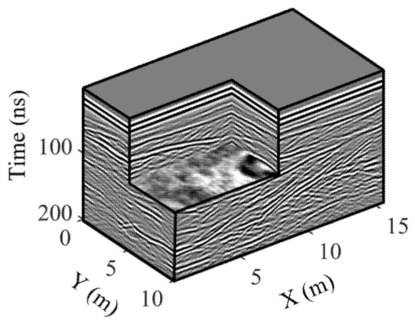
We first consider the application of our approach to a 100 MHz center-frequency synthetic GPR dataset called Herten, which was created via a 3D finite-difference-time-domain numerical simulation of Maxwell’s equations across a realistic fluvio-glacial aquifer analog model using the gprMax software (e.g., [41,42,43]). The electrical property distribution used to generate the synthetic GPR data is 16 m long by 10 m wide by 7 m deep. The corresponding high-resolution 3D dataset, which we consider our reference in this example, has a 0.1 m measurement spacing in the along-line (X) direction, a 0.1 m measurement spacing in the across-line (Y) direction, and a 0.337 ns time discretization. Figure 3 shows a 3D cutaway view of the high-resolution Herten volume after basic processing, which consisted of time-zero correction, de-wow, application of a smooth and time-varying gain, and low-pass filtering. We observe in the figure a complex combination of diffractions as well as reflections having different characteristic lengths and dip angles. The lack of horizontal continuity and short range of many of the reflections makes this dataset a challenging and realistic test case for our 3D reconstruction methodology.

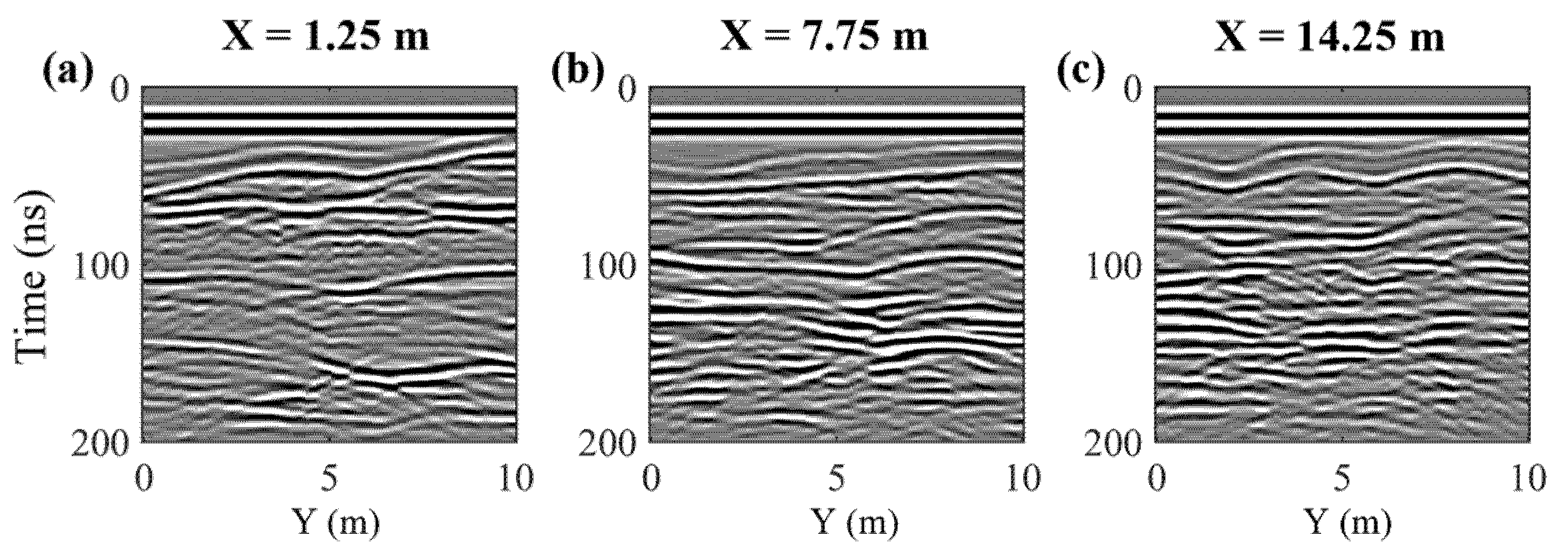
We consider two decimation cases with the Herten dataset (Table 1). In the first case, which we refer to as our moderate decimation example, survey lines were regularly removed from the volume presented in Figure 3 such that the measurement spacing in the across-line direction became 0.8 m. This amounts to deleting 87.5% of the total number of traces. In the second case, which we refer to as our severe decimation example, survey lines were removed such that the across-line spacing became 1.2 m, meaning the removal of 91.6% of the total number of traces. The decimated low-resolution datasets then served as the basis for our 3D reconstruction methodology, where the aim was to best estimate the original high-resolution volume. As mentioned above, three GPR profiles in the across-line direction were also considered to be available for the QS procedure and served as TIs for simulations conducted in that direction. These were located at along-line positions of X = 1.25 m, X = 7.75 m, and X = 14.25 m (Figure 4). The time required to generate one 3D realization with our QS methodology for the moderate and severe decimation examples, running on a workstation containing a 3 GHz Intel Xeon Gold 6248R CPU with 16 threads, was 1.7 h and 1.9 h, respectively (Table 2). For kriging along the time slices, the time required was 0.4 h and 0.3 h, respectively.

For each QS simulation for both the moderate and severe decimation examples, the parameter $N$ was set to 200 for the categorical volume reconstruction and to 50 for the final continuous volume reconstruction. These values were found to provide good replication of the structural reflection patterns and amplitude characteristics observed in the corresponding TIs, respectively. Following Zhang et al. (2024) [33], we began our testing with a value of $N=50$ for the categorical simulations but quickly found that the resulting profiles lacked realism compared to the TIs for the Herten dataset. As a result, $N$ was increased to the point where the categorical simulations were similar in character to the TIs. The latter was accomplished rapidly, as only a few 2D simulations were required for evaluation. Parameters $k$ and α in the QS algorithm were set to 1.1 and 0.02, respectively, as found by Zhang et al. [33] to provide high-quality simulation results with no verbatim copy from the TI, with similarly high-quality results here.

3.1.1. Moderate Decimation Example

Figure 5, Figure 6 and Figure 7 display the reconstruction results obtained for the decimated Herten dataset with an across-line measurement spacing of 0.8 m. In Figure 5, we examine the results for four selected across-line profiles, which are located at along-line positions of X = 0.25 m, 5.15 m, 10.15 m, and 15.65 m. The locations of these lines in the data cube are shown on the left, whereas the left, center, and right columns of the adjacent matrix display the original high-resolution data, the low-resolution decimated data, and the pixel-wise mean of 10 stochastic QS realizations, respectively. We see that when decimating the data by keeping only one of every eight traces, strong spatial aliasing is introduced. Indeed, many steeply dipping features such as diffraction tails seem to disappear, and the decimated across-line profiles show only a faint resemblance to the originals. In the reconstructed results, we observe that our proposed algorithm has done an impressive job of recovering most of the key reflection patterns. For instance, the strong, undulating reflection in the upper part of the domain from 30–70 ns, which is often difficult to follow in the decimated results, is accurately recovered in all four selected profiles. The same is true for two other variable reflecting interfaces located around 100 ns and 150 ns. There are some smaller-scale features in the original dataset, however, that our approach was not able to recover due to a complete lack of coherence of these features in the decimated dataset. Examples include the numerous diffraction hyperbolae appearing in Figure 5j between 100 and 150 ns, highlighted by the yellow box, and the deeper diffraction hyperbola occurring between 150 and 200 ns at a position of approximately y = 7.5 m in Figure 5a, outlined with the green box. Indeed, parts of these features remaining in the decimated dataset were reconstructed as shallowly dipping reflecting interfaces, which are predominant in the three across-line TIs shown in Figure 4.

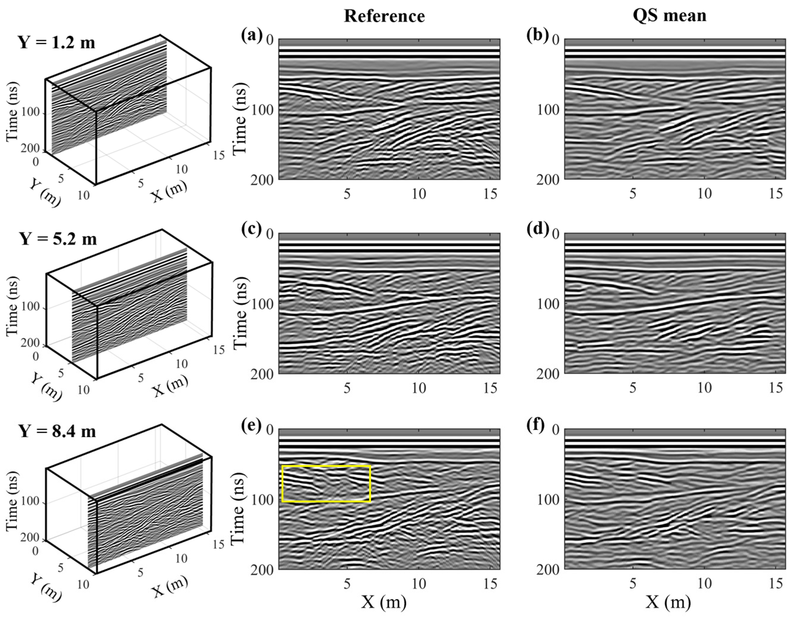
In Figure 6, we examine the reconstruction results along three selected along-line profiles, which are located at across-line positions of Y = 1.2 m, 5.2 m, and 8.4 m. Note that these profiles were entirely removed from the original high-resolution dataset and find themselves mid-way between the profile lines that were retained in the decimated volume. In this way, they represent reconstructions performed with a minimum number of conditioning data. As before, the locations of the lines in the data cube are shown on the left, whereas the left and right columns of the adjacent matrix contain the reference data and the pixel-wise mean of 10 stochastic QS realizations, respectively. We see in Figure 6 that the reconstructions show a remarkable degree of similarity with the corresponding reference profiles, which underscores the effectiveness of our proposed approach. All of the large-scale reflection structures have been accurately captured, and most of the shorter-length-scale dipping reflections, such as the cross-bedding present between 50 and 100 ns, are also well modeled. As was seen previously, some diffraction hyperbolae present in the original volume are missing in the reconstruction results, most notably on the left side of Figure 6e between 50 and 80 ns, as highlighted by the yellow box, but this is not surprising given the fact that the only conditioning information utilized to simulate these profiles was that coming from the across-line QS simulations.

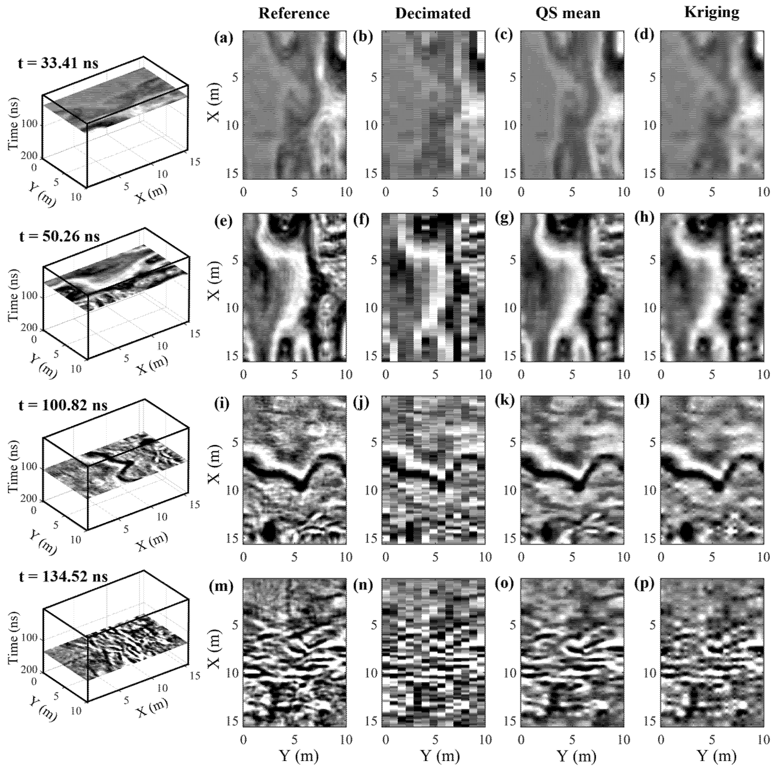
Finally, Figure 7 shows the reconstruction results obtained along four selected time slices located at t = 33.41 ns, 50.26 ns, 100.82 ns, and 134.52 ns. The positions of these slices in the data cube are again shown on the left side of the figure, whereas the adjacent matrix presents, from left to right, the original high-resolution data, the decimated data, the pixel-wise mean of 10 stochastic QS realizations, and the results of 2D time-slice interpolation using kriging. Again, the latter represents a common approach to densify 3D GPR datasets in the across-line direction. We see that each time-slice reconstruction obtained using our QS-based method is highly similar to the corresponding reference image, despite clear evidence of spatial aliasing in the decimated data. Most impressive are the accurate reconstructions of the multi-legged structures near the bottoms of Figure 7a,e, which are barely visible in the decimated images, and the strong and highly variable channel-like event in Figure 7i. The corresponding kriging interpolation results, on the other hand, are not nearly as impressive. The images are overall less sharp than the QS estimates, and the multi-legged structures in Figure 7a,e are not well captured. With regard to the channel-like event in Figure 7i, the general form is properly represented in the kriging result, but “staircasing” can be observed around Y = 7 m, where the feature slopes strongly in the across-line direction and is thus spatially aliased after decimation (Figure 7j). Finally, over all of the time slices, the kriged images exhibit many more localized point-like artifacts than the QS results, which may result from the nearest conditioning data having too strong an influence on these minimum-error-variance estimates and the fact that only two-point relationships have been taken into account.

To summarize, consideration of the 3D nature of the underlying reflection structures along with multiple-point patterns in our approach results in highly realistic results having strong advantages over kriging. To further explore this point, we consider the values of the RMSE, MAE, and SSIM metrics presented in Table 2, which again are global measures of how well the reconstructions compare with the original high-resolution reference data. The QS estimate exhibits a lower RMSE of 0.0619, compared to 0.0648 for kriging, whereas the MAE value for QS is marginally higher at 0.0375, compared to 0.0370 for kriging. This indicates that the use of the QS approach resulted in a slightly greater average error per point but a superior fit to the reference data in a least-squares sense, the latter most likely occurring because high-amplitude events, which may be related to important structures of interest, are better reconstructed. Concerning the SSIM metric, the QS approach outperforms kriging with a score of 0.6515 versus 0.6498, aligning with the previously noted observations from Figure 7 that the QS method more effectively captures the inherent structures and patterns of the original dataset.

3.1.2. Severe Decimation Example

Figure 8, Figure 9 and Figure 10 show the reconstruction results obtained for the decimated Herten dataset with an across-line measurement spacing of 1.2 m. Figure 8 presents the same across-line profiles considered in Figure 5, located at along-line positions of X = 0.25 m, 5.15 m, 10.15 m, and 15.65 m. Compared to our previous example, the greater degree of decimation in this case results in strong spatial aliasing. Not only do steeply dipping features such as diffraction tails seem to disappear, but many important reflection horizons also cannot be followed from one trace to another. Using the QS methodology, however, we are able to successfully recover the majority of the essential structures, albeit to a slightly lesser extent than in our moderate decimation example. Most notably, the undulating reflector in Figure 8j, occurring in the upper part of the profile from 30 to 50 ns, is remarkably well captured in the simulation results in Figure 8l, considering that it cannot be followed visually in the decimated results in Figure 8k. Similar to what we observed previously, many diffraction hyperbolae with steeply dipping tails, such as those highlighted by the yellow box in Figure 8j, are not reconstructed in the QS estimates but rather incorporated into reflecting interfaces, which are predominant in the three across-line TIs (Figure 4). Given the available measurements that were used to condition the simulations (e.g., Figure 8k), the proper recreation of such diffraction features is unlikely.

Figure 9 displays the reconstruction results for three selected along-line profiles, situated mid-way between profiles in the decimated volume at positions Y = 1.8 m, 5.4 m, and 7.8 m. We see that the QS estimates exhibit a high level of consistency with the reference profiles despite the fact that the only conditioning data for simulating these profiles were derived from QS simulations in the across-line direction. Indeed, all of the major reflection structures are well represented in the QS results, and numerous sets of short cross-bedding reflections, occurring between 50 and 90 ns, are also properly reconstructed. Some reconstruction challenges, however, are also observed that were not encountered in our moderate decimation case (Figure 6). For instance, the amplitudes in many parts of the reconstructed profiles are weaker than those in the reference volume (e.g., green box in Figure 9c), and the highly complex reflection structures observed in the lower-right region of all profiles are simplified (e.g., yellow boxes in Figure 9a,e). Information regarding the latter may be already lost through the across-line simulations and exacerbated by the lack of conditioning data for these simulations because of the greater spacing between the survey lines. Further, the averaging performed over 10 stochastic realizations to obtain our QS results, which again represent an MPS-based “best estimate” of the high-resolution dataset, has the effect of smoothing poorly constrained regions of the subsurface.

In Figure 10, we show the reconstruction results for the same four time slices considered in Figure 7, located at t = 33.41 ns, 50.26 ns, 100.82 ns, and 134.52 ns. As could be expected, significantly more spatial aliasing is observed in the decimated data for this example, which complicates considerably the time-slice reconstruction problem. Little correlation can be observed between the survey lines, and most of the structure seen in the original high-resolution images appears to be lost. Despite this, our developed QS procedure allows for a remarkable recovery of most of the key features in the reference slices, albeit slightly more smoothed for the reasons described above. For instance, the multi-legged structures near the bottoms of Figure 10a,e are reasonably well captured in Figure 10c,g, and the channel-like event in Figure 10i is recovered accurately in Figure 10k, with the exception of a discontinuity at around Y = 7 m. The same cannot be said for the results of kriging interpolation between the time slices. The kriging estimates are much smoother than those obtained in our moderate decimation example (Figure 7), and most of the structures in the images fail to be accurately recovered.

In summary, based on the visual inspection of Figure 8, Figure 9 and Figure 10, our proposed MPS-based 3D reconstruction approach proves highly effective in reconstructing the high-resolution reference volume, in particular compared to kriging, despite the fact that the severe degree of decimation in this case not only leads to a reduction in the number of conditioning data but also the number of available TIs. These observations are confirmed by the evaluation metrics presented in Table 2, which reveal that the QS estimate exhibits a lower RMSE of 0.0811 compared to 0.0857 for kriging interpolation, a marginally lower MAE of 0.0493 compared to 0.0500, and a higher SSIM index of 0.5356 compared to 0.5212.

3.2. Field Data Example: BHRS Dataset

As a final example, we apply our 3D reconstruction approach to a 200 MHz field dataset acquired at the Boise Hydrogeophysical Research Site (BHRS) located adjacent to the Boise River, Idaho, USA [44]. The full high-resolution data volume considered in this work, which represents the target for our reconstructions, is 30 m long by 18 m wide and covers a two-way travel time of 180 ns. The corresponding trace spacing in the along-line (X) and across-line (Y) directions is the same and equal to 0.1 m, and the time sampling interval is equal to 0.6 ns. Figure 11 presents a 3D cutaway view of the BHRS data cube following the same basic processing used in our synthetic example. Similar to before, we observe a mix of long- and short-range reflections at various orientations, along with numerous diffraction hyperbolae, which make this dataset an interesting and challenging test case for our 3D densification methodology.

For this reconstruction test, survey lines were regularly removed from the BHRS volume, leading to an across-line measurement spacing of 0.8 m. This represents the deletion of 87.5% of the total number of traces. The time required to generate one QS-based realization was approximately 2.7 h on the same workstation described previously, whereas kriging along time slices required 2.4 h. Similar to the Herten example, three GPR profiles in the across-line direction were also considered TIs for the QS simulations in that direction. These are located at along-line positions of X = 1 m, X = 15 m, and X = 29 m and presented in Figure 12. For both the categorical and continuous amplitude BHRS reconstructions, our initial value of $N=50$ was found to provide a good replication of the structural reflection patterns and amplitude characteristics of the TIs. Parameters $k$ and $\alpha$ were set to 1.1 and 0.02, respectively, which are the same values used with the Herten dataset.

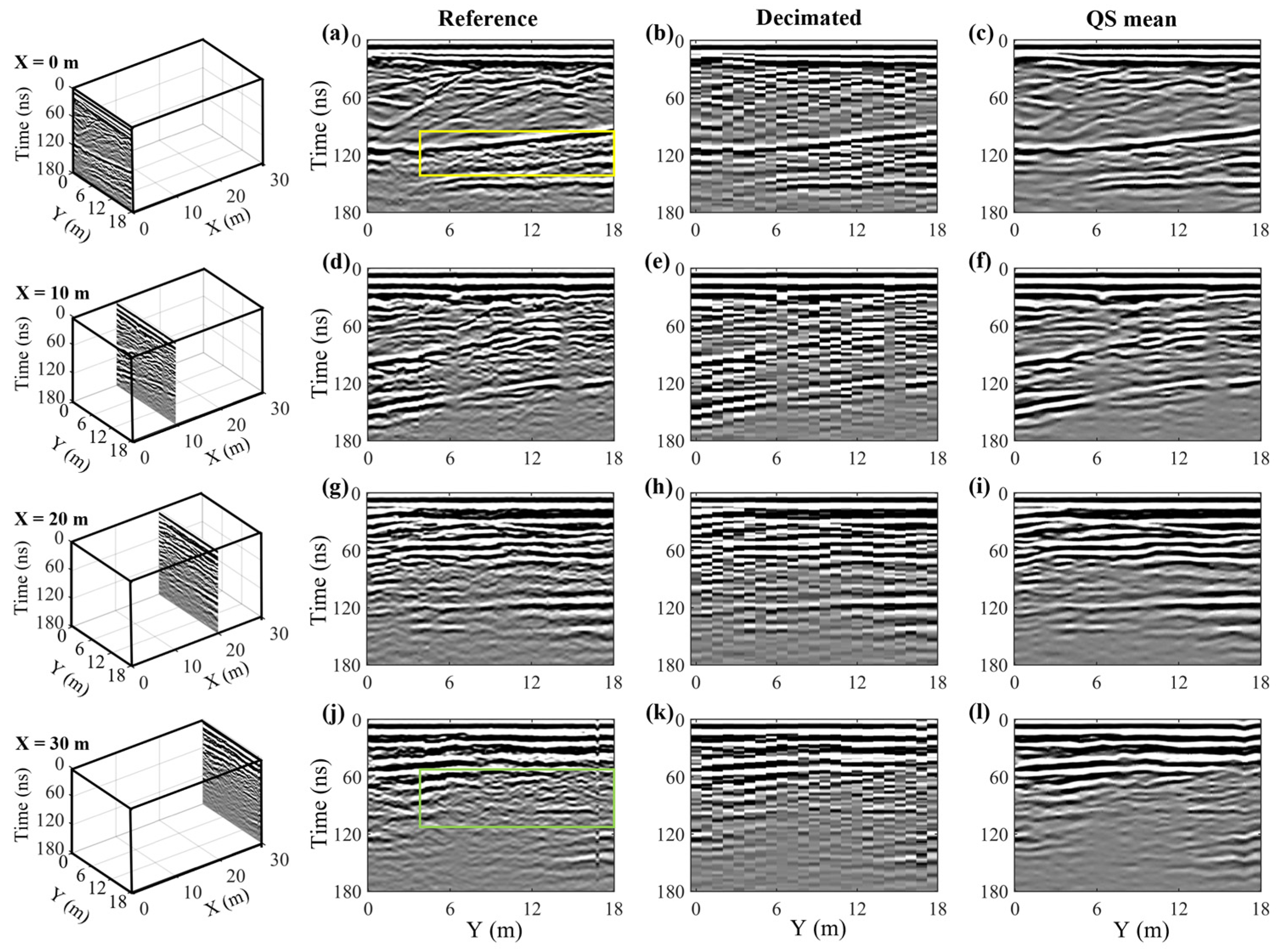
Figure 13 shows the BHRS reconstruction results for four selected across-line profiles, located at along-line positions of X = 0 m, 10 m, 20 m, and 30 m. The decimated images, particularly the dipping reflections in the upper part of Figure 13b, are strongly spatially aliased, but much of this is resolved in the corresponding QS estimates (e.g., Figure 13c). Indeed, most of the QS results show an excellent match with the reference profiles, with the exception of some zones containing multiple small-scale diffraction hyperbolae, for instance around 130 ns in Figure 13a, as highlighted by the yellow box, and between 60 and 120 ns in Figure 13j, as highlighted by the green box, which become more laterally smoothed in the corresponding reconstructions in Figure 13c,l. Again, the latter results in part from the fact that the presented QS reconstructions represent the mean of 10 stochastic realizations rather than a single realization of our 3D reconstruction procedure, which has the tendency to smooth features in zones that are less well constrained by the available data.

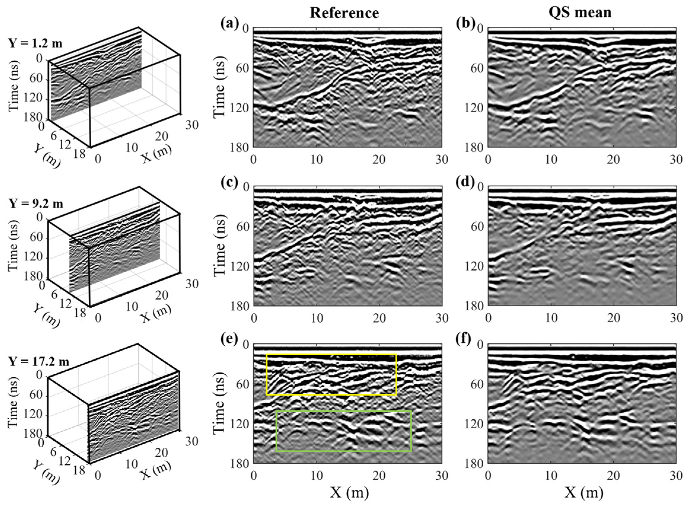
Figure 14 presents the BHRS reconstruction results for three selected along-line profiles, which are located mid-way between survey lines in the decimated dataset at across-line positions of Y = 1.2 m, 9.2 m, and 17.2 m. Similar to what was observed in Figure 13, all of the QS estimates can be seen to display a close match with the high-resolution reference profiles. For example, the dipping reflections at various angles in the left part of the three profiles, between approximately 60 and 120 ns, have been successfully captured, and larger diffraction hyperbolae, such as those present below 120 ns, are also well modeled. Again, however, some zones containing multiple superimposed small-scale diffraction features, as highlighted by the yellow and green boxes in Figure 14e, are laterally smoothed in the reconstruction results.

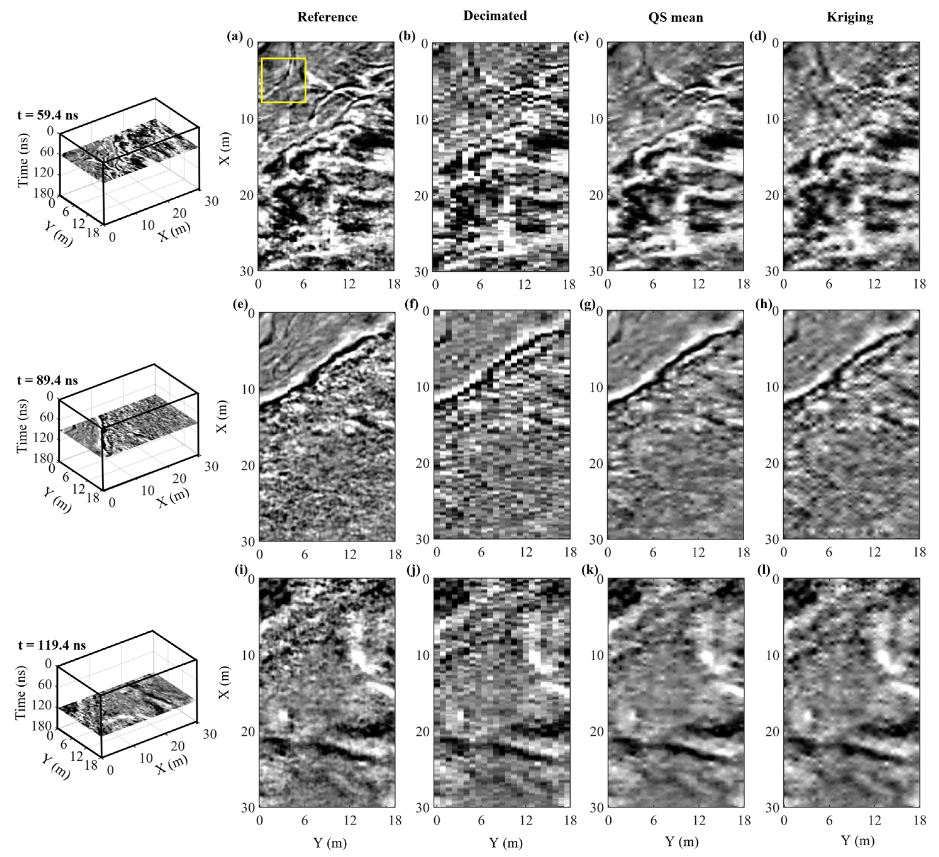
Three selected time-slice reconstructions for the BHRS dataset are presented in Figure 15, corresponding to t = 59.4 ns, 89.4 ns, and 119.4 ns. Similar to the Herten synthetic example, the QS results are compared to those obtained using 2D kriging interpolation along the time slices. The decimated time slices exhibit a high degree of spatial aliasing in some locations, most notably in the upper part of Figure 15b between X = 0 m and 10 m, where the reflection structures are hard to trace laterally from one line to another. The corresponding QS estimates manage to recover much of this structure and match well with the reference images (e.g., Figure 15c). However, some features at steep angles to the across-line direction are not reproduced, as illustrated by the yellow box in Figure 15a, and the results are noticeably smoother than the reference high-resolution data. Regarding the kriging interpolation results, more artifacts can be observed compared to the QS reconstructions. Most evident is the strong staircasing of steeply inclined features and the greater abundance of punctual anomalies. This being said, the differences between the kriging and QS results appear to be less severe for this example than for the Herten synthetic dataset.

Examining the metrics in Table 2 for the BHRS data, we observe a lower RMSE value of 0.5305 for the QS estimates compared to 0.5378 for kriging but a higher MAE value of 0.3201 compared 0.3153. Interestingly, the SSIM index value for the QS results is lower at 0.5957, compared to 0.6166 for kriging, which is puzzling given the moderately better visual fit observed in Figure 15. Again, this may result from the fact that the QS results represent the mean of 10 stochastic realizations, which has the effect of smoothing the reconstructed volume in regions less well constrained by the data.

4. Discussion and Conclusions

The primary objective of this work is to present a novel methodology for reconstructing a high-resolution 3D GPR data volume from measurements acquired along a set of sparsely spaced parallel profile lines. The reconstruction process is based on a series of 2D QS simulations, whereby randomly selected profiles are simulated along orthogonal orientations in an alternating manner. Such an approach, which was originally proposed by Comunian et al. [26] for MPS-based simulations of geological heterogeneity, helps to enforce 3D structural consistency in the output results while at the same time avoiding the need for a fully 3D simulation and a corresponding 3D TI, the latter of which is generally unavailable in the case of GPR data. One particular and important element of our approach, which greatly helps in generating more realistic structures, is the initial simulation of a high-resolution 3D categorical amplitude volume, which is then used as a secondary variable to guide the simulation of the continuous amplitude images. Our experience so far indicates that a value of $N=50$ represents a good starting point for this categorical simulation, after which a small number of simulated profiles can be compared with the categorical TIs to determine if an increase in $N$ is necessary. Once the overall reflection patterns were defined by the initial categorical simulation, we found that a value of $N=50$ for the final continuous amplitude simulations provided consistently excellent results. Setting parameters $k$ and $\alpha$ to 1.1 and 0.02, respectively, which was done for all of our examples and based on the work of Zhang et al. (2024) [33], was also found to produce high-quality reconstructions. Our methodology was successfully applied to both synthetic and field 3D GPR data under various decimation scenarios.

Computational efficiency is a crucial factor when considering the reconstruction of 3D data volumes. A key advantage of our algorithm is its operation entirely along 2D planes, thus avoiding the need for expensive 3D simulations and allowing for easy execution on a standard desktop computer. For all of the examples presented in this paper, which were carried out on a workstation containing an Intel Xeon Gold 6248R CPU with 16 threads, a single 3D stochastic realization was obtained in between 1.7 and 2.7 h. The proposed reconstruction procedure may be repeated multiple times to generate different realizations, which can then be used to assess the uncertainty of the reconstructed zones, especially in locations where constraints are weak. These realizations can also be averaged, as was done in this paper, to obtain an MPS-based best estimate of the high-resolution 3D volume. It should be noted that, for all of the examples presented here, differences between the 10 calculated stochastic realizations were found to be rather minor and limited to small-scale details. Clearly, however, these differences would be more significant in the case of further increases in the decimation rate.

For the synthetic Herten dataset, the MPS-based estimates of the high-resolution 3D GPR volume were shown both visually and via metrics to provide a generally superior result over standard 2D kriging interpolation along time slices for both our moderate and severe decimation examples. However, in the case of the BHRS field dataset, kriging was found to perform better in two of the three considered metrics (Table 2). Nevertheless, the results for the corresponding time slices (Figure 15) provided by our QS methodology show more realistic-looking outcomes. In all of our examples, the QS procedure took approximately one to six times longer to generate a single realization compared to kriging, and 10 of such realizations were averaged to obtain our final presented results. Despite the significantly increased computational expense of our method, we feel that the superior visual quality and realism shown by the QS results makes it worthwhile. However, more research and testing on a wide variety of other 3D GPR datasets is needed before any general conclusions can be made.

Another advantage of our proposed method is its ease of implementation. The QS simulation is typically controlled by three main parameters: $N$, α, and $k$. In our tests based on the Herten and BHRS datasets, selecting an appropriate value for $N$ requires some trial and error but is relatively straightforward and can be evaluated by comparing the simulated structures with the patterns in the TI. As for parameters $k$ and α, we maintained them at fixed values throughout our experiments and observed good results that were similar to the reference profiles.

One limitation in applying our proposed algorithm is having appropriate TIs in the across-line direction. In practice, multiple TIs exist for the along-line direction from the acquired GPR profiles, but either TIs for the across-line direction must be measured independently or it must be assumed that isotropy applies, allowing the use of along-line TIs for both directions. In the work presented in this paper, three additional crossline TIs were assumed to be available for QS simulations in this direction. These profiles, which require minimal effort in the field to acquire, were found to help the approach to generate highly realistic structures. In practice, however, most already existing 3D GPR datasets would not contain such profiles.

We are currently exploring the use of deep-learning-based tools for 3D GPR trace reconstruction, which have gained increasing popularity in recent years for both GPR and seismic applications. After proper training of the corresponding convolutional neural network, these tools could offer a highly computationally efficient means of simulating data in the along-line and across-line directions, thereby permitting the application of the approach considered here to larger 3D GPR datasets, such as those recently acquired by drones over glaciers [45]. Part of this work involves investigating whether, by considering a rich training database consisting not only of the available along-line profiles but also synthetically generated datasets, we can reduce the dependency on the additional collection of across-line TIs. This could further improve the reconstruction performance of existing 3D GPR datasets where such profiles are unavailable.

References

1. Annan, A.P. Ground-Penetrating Radar. In Near-Surface Geophysics; Society of Exploration Geophysicists: Tulsa, OK, USA, 2005; pp. 357–438. [Google Scholar]
2. Knight, R. Ground Penetrating Radar for Environmental Applications. Annu. Rev. Earth Planet. Sci. 2001, 29, 229–255. [Google Scholar] [CrossRef]
3. Grasmueck, M.; Weger, R.; Horstmeyer, H. Full-resolution 3D GPR imaging. Geophysics 2005, 70, K12–K19. [Google Scholar] [CrossRef]
4. Leucci, G.; De Giorgi, L.; Di Giacomo, G.; Ditaranto, I.; Miccoli, I.; Scardozzi, G. 3D GPR survey for the archaeological characterization of the ancient Messapian necropolis in Lecce, South Italy. J. Archaeol. Sci. Rep. 2016, 7, 290–302. [Google Scholar] [CrossRef]
5. Novo, A.; Grasmueck, M.; Viggiano, D.; Lorenzo, H. 3D GPR in archaeology: What can be gained from dense data acquisition and processing. In Proceedings of the 12th International Conference on Ground Penetrating Radar, Birmingham, UK, 15–19 June 2008. [Google Scholar]
6. Molron, J.; Linde, N.; Baron, L.; Selroos, J.-O.; Darcel, C.; Davy, P. Which fractures are imaged with Ground Penetrating Radar? Results from an experiment in the Äspö Hardrock Laboratory, Sweden. Eng. Geol. 2020, 273, 105674. [Google Scholar] [CrossRef]
7. Church, G.; Bauder, A.; Grab, M.; Maurer, H. Ground-penetrating radar imaging reveals glacier’s drainage network in 3D. Cryosphere 2021, 15, 3975–3988. [Google Scholar] [CrossRef]
8. Egli, P.E.; Irving, J.; Lane, S.N. Characterization of subglacial marginal channels using 3-D analysis of high-density ground-penetrating radar data. J. Glaciol. 2021, 67, 759–772. [Google Scholar] [CrossRef]
9. Liu, Z.; Yeoh, J.K.; Gu, X.; Dong, Q.; Chen, Y.; Wu, W.; Wang, L.; Wang, D. Automatic pixel-level detection of vertical cracks in asphalt pavement based on GPR investigation and improved mask R-CNN. Autom. Constr. 2023, 146, 104689. [Google Scholar] [CrossRef]
10. Liu, Z.; Wu, W.; Gu, X.; Li, S.; Wang, L.; Zhang, T. Application of combining YOLO models and 3D GPR images in road detection and maintenance. Remote Sens. 2021, 13, 1081. [Google Scholar] [CrossRef]
11. Allroggen, N.; Booth, A.D.; Baker, S.E.; Ellwood, S.A.; Tronicke, J. High-resolution imaging and monitoring of animal tunnels using 3D ground-penetrating radar. Near Surf. Geophys. 2019, 17, 291–298. [Google Scholar] [CrossRef]
12. Saey, T.; Van Meirvenne, M.; De Pue, J.; Van De Vijver, E.; Delefortrie, S. Reconstructing mole tunnels using frequency-domain ground penetrating radar. Appl. Soil Ecol. 2014, 80, 77–83. [Google Scholar] [CrossRef]
13. Gaballah, M.; Grasmueck, M.; Sato, M. Characterizing subsurface archaeological structures with full resolution 3D GPR at the early dynastic foundations of Saqqara Necropolis, Egypt. Sens. Imaging 2018, 19, 23. [Google Scholar] [CrossRef]
14. Booth, A.D.; Linford, N.T.; Clark, R.A.; Murray, T. Three-dimensional, multi-offset ground-penetrating radar imaging of archaeological targets. Archaeol. Prospect. 2008, 15, 93–112. [Google Scholar] [CrossRef]
15. Spitz, S. Seismic trace interpolation in the FX domain. Geophysics 1991, 56, 785–794. [Google Scholar] [CrossRef]
16. Topczewski, L.; Fernandes, F.M.; Cruz, P.J.; Lourenço, P.B. Practical implications of GPR investigation using 3D data reconstruction and transmission tomography. J. Build. Apprais. 2007, 3, 59–76. [Google Scholar] [CrossRef]
17. Samet, R.; Çelik, E.; Tural, S.; Şengönül, E.; Özkan, M.; Damcı, E. Using interpolation techniques to determine the optimal profile interval in ground-penetrating radar applications. J. Appl. Geophys. 2017, 140, 154–167. [Google Scholar] [CrossRef]
18. Rucka, M.; Wojtczak, E.; Zielińska, M. Interpolation methods in GPR tomographic imaging of linear and volume anomalies for cultural heritage diagnostics. Measurement 2020, 154, 107494. [Google Scholar] [CrossRef]
19. Goodman, D.; Piro, S. GPR Remote Sensing in Archaeology; Springer: New York, NY, USA, 2013. [Google Scholar]
20. Luo, T.X.; Lai, W.W.; Chang, R.K.; Goodman, D. GPR imaging criteria. J. Appl. Geophys. 2019, 165, 37–48. [Google Scholar] [CrossRef]
21. Verdonck, L.; Taelman, D.; Vermeulen, F.; Docter, R. The Impact of Spatial Sampling and Migration on the Interpretation of Complex Archaeological Ground-penetrating Radar Data. Archaeol. Prospect. 2015, 22, 91–103. [Google Scholar] [CrossRef]
22. Abma, R.; Kabir, N. 3D interpolation of irregular data with a POCS algorithm. Geophysics 2006, 71, E91–E97. [Google Scholar] [CrossRef]
23. Gülünay, N. Seismic trace interpolation in the Fourier transform domain. Geophysics 2003, 68, 355–369. [Google Scholar] [CrossRef]
24. Kabir, M.N.; Verschuur, D. Restoration of missing offsets by parabolic radon transform. Geophys. Prospect. 1995, 43, 347–368. [Google Scholar] [CrossRef]
25. Mariethoz, G.; Caers, J. Multiple-Point Geostatistics: Stochastic Modeling with Training Images; John Wiley & Sons: Hoboken, NJ, USA, 2014. [Google Scholar]
26. Comunian, A.; Renard, P.; Straubhaar, J. 3D multiple-point statistics simulation using 2D training images. Comput. Geosci. 2012, 40, 49–65. [Google Scholar] [CrossRef]
27. Strebelle, S. Conditional simulation of complex geological structures using multiple-point statistics. Math. Geol. 2002, 34, 1–21. [Google Scholar] [CrossRef]
28. Rasera, L.G.; Gravey, M.; Lane, S.N.; Mariethoz, G. Downscaling images with trends using multiple-point statistics simulation: An application to digital elevation models. Math. Geosci. 2020, 52, 145–187. [Google Scholar] [CrossRef]
29. Tang, Y.; Zhang, J.; Jing, L.; Li, H. Digital elevation data fusion using multiple-point geostatistical simulation. IEEE J. Sel. Top. Appl. Earth Obs. Remote Sens. 2015, 8, 4922–4934. [Google Scholar] [CrossRef]
30. Hadjipetrou, S.; Mariethoz, G.; Kyriakidis, P. Gap-filling sentinel-1 offshore wind speed image time series using multiple-point geostatistical simulation and reanalysis data. Remote Sens. 2023, 15, 409. [Google Scholar] [CrossRef]
31. Yin, G.; Mariethoz, G.; McCabe, M.F. Gap-filling of landsat 7 imagery using the direct sampling method. Remote Sens. 2016, 9, 12. [Google Scholar] [CrossRef]
32. Oriani, F.; Straubhaar, J.; Renard, P.; Mariethoz, G. Simulation of rainfall time series from different climatic regions using the direct sampling technique. Hydrol. Earth Syst. Sci. 2014, 18, 3015–3031. [Google Scholar] [CrossRef]
33. Zhang, C.; Gravey, M.; Mariéthoz, G.; Irving, J. Reconstruction of missing GPR data using multiple-point statistical simulation. IEEE Trans. Geosci. Remote Sens. 2024, 62, 1–17. [Google Scholar] [CrossRef]
34. Guardiano, F.B.; Srivastava, R.M. Multivariate geostatistics: Beyond bivariate moments. In Geostatistics Tróia’92: Volume 1; Springer: Dordrecht, The Netherlands, 1993; pp. 133–144. [Google Scholar]
35. Straubhaar, J.; Renard, P.; Mariethoz, G.; Froidevaux, R.; Besson, O. An improved parallel multiple-point algorithm using a list approach. Math. Geosci. 2011, 43, 305–328. [Google Scholar] [CrossRef]
36. Mariethoz, G.; Renard, P.; Straubhaar, J. The direct sampling method to perform multiple-point geostatistical simulations. Water Resour. Res. 2010, 46, W11536. [Google Scholar] [CrossRef]
37. Gravey, M.; Mariethoz, G. QuickSampling v1. 0: A robust and simplified pixel-based multiple-point simulation approach. Geosci. Model Dev. 2020, 13, 2611–2630. [Google Scholar] [CrossRef]
38. Gueting, N.; Caers, J.; Comunian, A.; Vanderborght, J.; Englert, A. Reconstruction of three-dimensional aquifer heterogeneity from two-dimensional geophysical data. Math. Geosci. 2018, 50, 53–75. [Google Scholar] [CrossRef]
39. Wang, Z.; Bovik, A.C.; Sheikh, H.R.; Simoncelli, E.P. Image quality assessment: From error visibility to structural similarity. IEEE Trans. Image Process. 2004, 13, 600–612. [Google Scholar] [CrossRef] [PubMed]
40. Isaaks, E.H.; Srivastava, R.M. An Introduction to Applied Geostatistics; Oxford University Press: New York, NY, USA, 1989. [Google Scholar]
41. Comunian, A.; Renard, P.; Straubhaar, J.; Bayer, P. Three-dimensional high resolution fluvio-glacial aquifer analog–Part 2: Geostatistical modeling. J. Hydrol. 2011, 405, 10–23. [Google Scholar] [CrossRef]
42. Koyan, P.; Tronicke, J. 3D modeling of ground-penetrating radar data across a realistic sedimentary model. Comput. Geosci. 2020, 137, 104422. [Google Scholar] [CrossRef]
43. Warren, C.; Giannopoulos, A.; Giannakis, I. gprMax: Open source software to simulate electromagnetic wave propagation for Ground Penetrating Radar. Comput. Phys. Commun. 2016, 209, 163–170. [Google Scholar] [CrossRef]
44. Bradford, J.H.; Clement, W.P.; Barrash, W. Estimating porosity with ground-penetrating radar reflection tomography: A controlled 3-D experiment at the Boise Hydrogeophysical Research Site. Water Resour. Res. 2009, 45, W00D26. [Google Scholar] [CrossRef]
45. Ruols, B.; Baron, L.; Irving, J. Development of a drone-based ground-penetrating radar system for efficient and safe 3D and 4D surveying of alpine glaciers. J. Glaciol. 2023, 1–12. [Google Scholar] [CrossRef]
Figure 1. Flowchart of the general QS MPS simulation approach.
Remotesensing 16 02084 g001
Figure 2. Workflow of the QS-based 3D GPR data reconstruction methodology. (a) Categorical GPR amplitude dataset derived from the original measurements, where a small number of across-line categorical profiles (red) are simulated at regular intervals. (b) Simulation of alternating, randomly selected, along-line and across-line categorical profiles conditional to all measured and previously simulated data. (c) Final high-resolution 3D categorical volume, which is paired with (d) the corresponding low-resolution continuous GPR measurements. A small number of across-line continuous profiles are simulated, guided by the categorical results. (e) Simulation of alternating, randomly selected, along-line and across-line continuous profiles. (f) Final high-resolution continuous 3D GPR volume.
Remotesensing 16 02084 g002
Figure 3. Reference high-resolution Herten synthetic dataset. The measurement spacing in the along-line (X) and across-line (Y) directions is the same and equal to 0.1 m.
Remotesensing 16 02084 g003
Figure 4. (ac) Three high-resolution across-line profiles from the Herten data cube presented in Figure 3, corresponding to along-line positions of X = 1.25 m, 7.75 m, and 14.25 m, respectively, which were considered TIs for the QS simulations in the across-line direction.
Remotesensing 16 02084 g004
Figure 5. (a,d,g,j) High-resolution across-line profiles from the Herten data cube presented in Figure 3 at along-line positions of X = 0.25 m, 5.15 m, 10.15 m, and 15.65 m, respectively. The positions of the profiles in the cube are shown in the left column, and the spatial sampling interval is equal to 0.1 m. (b,e,h,k) Corresponding decimated across-line profiles, where the spatial sampling interval has been reduced to 0.8 m. (c,f,i,l) Corresponding profiles from the reconstructed data cube, obtained via the mean of 10 stochastic QS realizations, where the reconstructed spatial sampling interval is 0.1 m.
Remotesensing 16 02084 g005
Figure 6. (a,c,e) High-resolution along-line profiles from the Herten data cube presented in Figure 3 at across-line positions of Y = 1.2 m, 5.2 m, and 8.4 m, respectively. The positions of the profiles in the cube are shown in the left column, and the spatial sampling interval is equal to 0.1 m. (b,d,f) Corresponding profiles from the reconstructed data cube, obtained via the mean of 10 stochastic QS realizations, where the reconstructed spatial sampling interval is 0.1 m. Note that in this case, the decimated along-line profiles do not exist.
Remotesensing 16 02084 g006
Figure 7. (a,e,i,m) High-resolution time slices from the Herten data cube presented in Figure 3 at t = 33.41 ns, 50.26 ns, 100.82 ns, and 134.52 ns, respectively. The positions of the profiles in the cube are shown in the left column, and the spatial sampling interval is equal to 0.1 m in both directions. (b,f,j,n) Corresponding decimated time slices, where the spatial sampling in the across-line (Y) direction has been reduced to 0.8 m. (c,g,k,o) Corresponding time slices from the reconstructed data cube, obtained via the mean of 10 stochastic QS realizations, where the reconstructed spatial sampling interval is 0.1 m in both directions. (d,h,l,p) Corresponding time slices from the reconstructed data cube obtained via kriging interpolation along the time slices.
Remotesensing 16 02084 g007
Figure 8. (a,d,g,j) High-resolution across-line profiles from the Herten data cube presented in Figure 3 at along-line positions of X = 0.25 m, 5.15 m, 10.15 m, and 15.65 m, respectively. The positions of the profiles in the cube are shown in the left column, and the spatial sampling interval is equal to 0.1 m. (b,e,h,k) Corresponding decimated across-line profiles, where the spatial sampling interval has been reduced to 1.2 m. (c,f,i,l) Corresponding profiles from the reconstructed data cube, obtained via the mean of 10 stochastic QS realizations, where the reconstructed spatial sampling interval is 0.1 m.
Remotesensing 16 02084 g008
Figure 9. (a,c,e) High-resolution along-line profiles from the Herten data cube presented in Figure 3 at across-line positions of Y = 1.8 m, 5.4 m, and 7.8 m, respectively. The positions of the profiles in the cube are shown in the left column, and the spatial sampling interval is equal to 0.1 m. (b,d,f) Corresponding profiles from the reconstructed data cube, obtained via the mean of 10 stochastic QS realizations, where the reconstructed spatial sampling interval is 0.1 m. Note that in this case, the decimated along-line profiles do not exist.
Remotesensing 16 02084 g009
Figure 10. (a,e,i,m) High-resolution time slices from the Herten data cube presented in Figure 3 at t = 33.41 ns, 50.26 ns, 100.82 ns, and 134.52 ns, respectively. The positions of the profiles in the cube are shown in the left column, and the spatial sampling interval is equal to 0.1 m in both directions. (b,f,j,n) Corresponding decimated time slices, where the spatial sampling in the across-line (Y) direction has been reduced to 1.2 m. (c,g,k,o) Corresponding time slices from the reconstructed data cube, obtained via the mean of 10 stochastic QS realizations, where the reconstructed spatial sampling interval is 0.1 m in both directions. (d,h,l,p) Corresponding time slices from the reconstructed data cube obtained via kriging interpolation along the time slices.
Remotesensing 16 02084 g010
Figure 11. Reference high-resolution BHRS field dataset. The measurement spacing in the along-line (X) and across-line (Y) directions is the same and equal to 0.1 m.
Remotesensing 16 02084 g011
Figure 12. (ac) Three high-resolution across-line profiles from the BHRS data cube presented in Figure 11, corresponding to along-line positions of X = 1 m, 15 m, and 29 m, respectively, which were considered TIs for the QS simulations in the across-line direction.
Remotesensing 16 02084 g012
Figure 13. (a,d,g,j) High-resolution across-line profiles from the BHRS data cube presented in Figure 11 at along-line positions of X = 0 m, 10 m, 20 m, and 30 m, respectively. The positions of the profiles in the cube are shown in the left column, and the spatial sampling interval is equal to 0.1 m. (b,e,h,k) Corresponding decimated across-line profiles, where the spatial sampling interval has been reduced to 0.8 m. (c,f,i,l) Corresponding profiles from the reconstructed data cube, obtained via the mean of 10 stochastic QS realizations, where the reconstructed spatial sampling interval is 0.1 m.
Remotesensing 16 02084 g013
Figure 14. (a,c,e) High-resolution along-line profiles from the BHRS data cube presented in Figure 11 at across-line positions of Y = 1.2 m, 9.2 m, and 17.2 m, respectively. The positions of the profiles in the cube are shown in the left column, and the spatial sampling interval is equal to 0.1 m. (b,d,f) Corresponding profiles from the reconstructed data cube, obtained via the mean of 10 stochastic QS realizations, where the reconstructed spatial sampling interval is 0.1 m. Note that in this case, the decimated along-line profiles do not exist.
Remotesensing 16 02084 g014
Figure 15. (a,e,i) High-resolution time slices from the BHRS data cube presented in Figure 11 at t = 59.4 ns, 89.4 ns, and 119.4 ns, respectively. The positions of the profiles in the cube are shown in the left column, and the spatial sampling interval is equal to 0.1 m in both directions. (b,f,j) Corresponding decimated time slices, where the spatial sampling in the across-line (Y) direction has been reduced to 0.8 m. (c,g,k) Corresponding time slices from the reconstructed data cube, obtained via the mean of 10 stochastic QS realizations, where the reconstructed spatial sampling interval is 0.1 m in both directions. (d,h,l) Corresponding time slices from the reconstructed data cube obtained via kriging interpolation along the time slices.
Remotesensing 16 02084 g015