Deep Learning Hyperspectral Pansharpening on Large-Scale PRISMA Dataset

Abstract

Hyperspectral pansharpening is crucial for the improvement of the usability of images in various applications. However, it remains underexplored due to a scarcity of data. The primary goal of pansharpening is to enhance the spatial resolution of hyperspectral images by reconstructing missing spectral information without compromising consistency with the original data. This paper addresses the data gap by presenting a new hyperspectral dataset specifically designed for pansharpening and the evaluation of several deep learning strategies using this dataset. The new dataset has two crucial features that make it invaluable for deep learning hyperspectral pansharpening research. (1) It presents the highest cardinality of images in the state of the art, making it the first statistically relevant dataset for hyperspectral pansharpening evaluation, and (2) it includes a wide variety of scenes, ensuring robust generalization capabilities for various approaches. The data, collected by the ASI PRISMA satellite, cover about 262,200 km² and their heterogeneity is ensured by a random sampling of the Earth’s surface. The analysis of the deep learning methods consists in the adaptation of these approaches to the PRISMA hyperspectral data and the quantitative and qualitative evaluation of their performance in this new scenario. The investigation included two settings: Reduced Resolution (RR) to evaluate the techniques in a controlled environment and Full Resolution (FR) for a real-world evaluation. In addition, for the sake of completeness, we have also included machine-learning-free approaches in both scenarios. Our comprehensive analysis reveals that data-driven neural network methods significantly outperform traditional approaches, demonstrating a superior adaptability and performance in hyperspectral pansharpening under both RR and FR protocols.

1. Introduction

Remote sensing (RS) has revolutionized our ability to observe and analyze our planet from a vantage point beyond the Earth’s surface [1]. The analysis of data gathered by sensors onboard satellites or aircraft, in fact, allows the inference of useful information about the land, water, and atmospheric systems of the Earth. This technology has become fundamental in several fields, such as environmental monitoring [2,3], agriculture [4], urban planning [5], disaster management [6], and resource exploration [7].

However, the costs of sending a satellite into Earth orbit are very high. They range from USD 2.6 k/kg with SpaceX to USD 22 k/kg with NASA, with an intermediate value of USD 17.6 k/kg with Soyuz, the Russian rocket system [8,9]. Minimizing the payload is therefore the major goal that drives the choice and the design of every component on a satellite [10]. This constraint, in combination with the need to use as little energy as possible, results in a huge trade-off between the spatial resolution and the number of acquired bands when designing optical remote sensing devices. On the one hand, in fact, several orbital expeditions, such as Landsat 6/7 [11], SPOT 6/7 [12], and Sentinel-2 [13], include a panchromatic imaging device acquiring data at high resolution [14]. On the other hand, missions carrying hyperspectral (HS) imaging devices, such as ASI PRISMA https://www.asi.it/scienze-della-terra/prisma/, accessed on 26 May 2024, have had to decrease the spatial resolution in favor of a higher number of acquired bands [15].

In this respect, the loss of spatial resolution can be partially solved through the use of pansharpening [16]. In this context, the panchromatic image is used as a source of information to extend the spatial resolution of the multispectral (MS) and HS images.

The first attempts at image pansharpening were provided by machine-learning-free approaches [17], designed to handle data in the range of visible radiations (400–700 nm). Among these methods, different groups of techniques, such as component substitution methods (CS), multiresolution analysis (MRA), Bayesian approaches, and matrix factorization techniques, can be recognized [18]. In the first group, the core idea is to use the projection of a high-resolution version of the spectral image into its spatial component and then revert the transformation using the panchromatic information instead of the extracted spatial projection. These methods are usually easy to implement, achieve a high spatial fidelity, and are robust to misregistration, but they can create significant spectral distortions [18]. Principal component analysis (PCA) [19], intensity–hue–saturation (IHS) [20], Gram–Schmidt (GS) [21], and GS Adaptive (GSA) [22] are all included in this group. The MRA group comprises the Decimated Wavelet Transform (DWT) [23], Undecimated Wavelet Transform (UDWT) [24], “à-trous” wavelet transform (ATWT) [25], and Laplacian Pyramid [26]. They typically consist in using a filtered version of the PAN signal to extract high-resolution details and inject them into the spectral image. Compared to the CS methods, the MRA techniques are more difficult to implement and computationally more complex, but also achieve a better spectral consistency with the original spectral information. Some other approaches, for instance, Guided Filter PCA [27], combine the two techniques to extract the advantages from each but the results on HS images have not been promising, being the technique with the worst results on HS data in Loncan et al.’s investigation [18]. The Bayesian approaches are based on the estimation of the posterior probability of the full-resolution image that would be obtained considering the original panchromatic and spectral information. These methods typically consider the sensor characteristics to enhance the resolution, thus achieving good results but also being less generalizable and more complex to use [18]. Finally, matrix factorization techniques are described by Loncan et al. [18] as the only ones purposely used for HS pansharpening, and instead of using the panchromatic information, they use a high-resolution MS image to convey the spatial information of the HS data into a higher-resolution space. Even in this case, to exploit the best factorization to reconstruct the new image, the characteristics of the sensors are taken into consideration, making them less viable compared to the other methods.

These machine-learning-free approaches assume the possibility of exploiting the existing relationship between the panchromatic image and the spectral bands in the input data. However, this assumption may not be valid when handling data outside the range of visible wavelengths, i.e., when there is a partial or missing spectral overlap between the panchromatic image and the spectral bands to be processed. Alongside these methods, neural network-based approaches have been recently developed, showing promising results even outside the visible part of the spectrum.

When it comes to deep learning approaches, most of the methodologies are based on MS data [28]. Nonetheless, some attempts in HS pansharpening have been proposed. In 2019, He at al. [29] proposed HyperPNN, a CNN that, firstly, extracts spatial features from the panchromatic image and spectral features from the HS image, secondly fuses the spatial and spectral features with dedicated convolutional layers, and thirdly predicts the spectral information of the pansharpened image with convolutional layers that focus only on the spectral signatures. This model was followed in 2020 by the improved version HySpecNet [30]. In the same year that HyperPNN was proposed, Zheng et al. [31] investigated the use of the residual network for pansharpening, firstly guiding the upscaling and enhancing the edge details of the HS data with Contrast Limited Adaptive Histogram Equalization (CLAHE) and a guided filter to fuse the image with the panchromatic information, and then using a Deep Residual Convolutional Neural Network (DRCNN) to boost the reconstruction. Xie et al. [32] developed the HS pansharpening method with Deep Priors (HPDP), exploiting the power of different deep learning modules to improve all parts of the pansharpening pipeline. In particular, they used a Super Resolution Deep Learning (SRDL) module to upscale the HS image and fuse it with the panchromatic information by also considering high-frequency information extracted by the proposed High-Frequency Net (HFNet). In the end, they obtained the final high-resolution HS image by injecting the high-frequency structure in the upscaled HS image, using a Sylvester equation. It is worth noticing that they used MS images for the training to compensate for the limited number of training samples. Recently, in 2023, He et al. [33] proposed dynamic HS pansharpening that uses a learn-to-learn strategy to adapt the pansharpening to the spatial variations of an image. Zhao et al. [34] proposed a generative adversarial network with a fast guided filter [35] for pansharpening, aiming to reduce the computational costs and retain the spatial information more effectively by highlighting the fusion objects with a spatial attention module and preserving the latent feature information through adversarial training. Zhu et al. [36] introduced a probability-based global cross-modal upsampling (PGCU) technique for pansharpening that leverages global and cross-modal information. The PGCU module includes information extraction, distribution and expectation estimation, and fine adjustment blocks, showing improvements in performance and enhancing existing deep learning pansharpening methods.

Despite the increased adoption of CNNs and deep learning in the field of pansharpening and the increased interest in using HS images for satellite image analysis, the limited number of HS samples is still an issue. Deep learning techniques, in fact, are data-driven approaches with the necessity of a high cardinality and high variability of the datasets. This necessity is a crucial problem in HS pansharpening because the majority of the existing datasets are not suitable for neural network training. Table 1 reports the most relevant datasets in the literature used for MS and HS RS pansharpening. It is possible to divide the existing datasets into different groups by mainly considering three properties: the wavelength coverage, image resolution, and acquisition set-up of each dataset. Regarding the wavelength coverage, four datasets present information from the visible to near-infra-red (VNIR) part of the spectrum, while the remaining ones cover the entire spectrum, from visible to short-wave infrared (SWIR). Data with a limited spectral coverage for the design of pansharpening algorithms could limit their applicability to real-world scenarios, which may require the use of bands and data not covered by those datasets. Another important aspect is the image resolution, which is associated with the dataset cardinality. The majority of these are composed of only one single satellite or aerial image covering a small portion of land (at most a few km²), with a limited variability in the content of the scene. While datasets like Halls Creek [30] can potentially be tiled in smaller samples for training or validation purposes, the other ones are limited due to their low cardinality and low resolution. Furthermore, even if an image is tiled, the variety of the content of the scenes considered is limited to the area covered by the single image, making it hard to evaluate algorithms in different scenarios. Finally, most of the datasets in the state-of-the-art are tagged as “airborne”, which means they are collected by using airplanes or low-altitude flying devices, while only two are made of satellite-collected images.

The characteristics of these data limit not only the performance of deep learning approaches but also our ability to properly evaluate their performance. The datasets have both a low sample cardinality, which is not statistically relevant for a proper evaluation, and a low variability, which makes the model unsuitable for different environments, consequently restricting the generalization capabilities of these approaches.

In order to overcome these limitations, in this paper, we present the following:

• A new large-scale dataset covering 262,200 km² for the qualitative assessment of deep neural models for HS image pansharpening. Such a dataset, compared with the others in Table 1, is collected from the PRISMA satellite, preprocessed and adopted for the retraining of current state-of-the-art approaches for image pansharpening.
• An in-depth statistically relevant comparison, both in quantitative and qualitative terms, of traditional machine-learning-free approaches and current deep learning approaches, adapted to HS data, retrained and tested on the newly proposed large-scale dataset.

To the best of our knowledge, the study presented is the first one based on a large-scale dataset, covering a wide variety of ground areas. Although other studies have investigated the problem of HS pansharpening, they have limited their analysis to a small number of samples and therefore are not able to clarify the real quality of the tested methods [37]. We believe that the proposed investigation will be a starting point for the design of new deep learning approaches for RS image pansharpening.

Table 1. List of existing datasets used for RS image pansharpening. For each dataset, the number of images of the dataset, the number of bands, and the coverage in terms of wavelength are here reported. The image resolutions presented in this table are taken from the original dataset descriptions.

Dataset	Cardinality	Images Resolution	Type	# of Bands	Wavelength Coverage
Pavia University	1	610 × 610	airborne	103	430–838 nm
Pavia Center	1	1096 × 1096	airborne	102	430–860 nm
Houston [33,38]	1	349 × 1905	airborne	144	364–1046 nm
Chikusei [39]	1	2517 × 2335	airborne	128	363–1018 nm
AVIRIS Moffett Field [18]	1	37 × 79	airborne	224	400–2500 nm
Garons [18]	1	80 × 80	airborne	125	400–2500 nm
Camargue [18]	1	100 × 100	airborne	125	400–2500 nm
Indian Pines [40]	1	145 × 145	airborne	224	400–2500 nm
Cuprite Mine	1	400 × 350	airborne	185	400–2450 nm
Salinas	1	512 × 217	airborne	202 (224)	400–2500 nm
Washington Mall [29]	1	1200 × 300	airborne	191 (210)	400–2400 nm
Merced [33]	1	180 × 180	satellite	134 (242)	400–2500 nm
Halls Creek [30]	1	3483 × 567	satellite	171 (230)	400–2500 nm
OURS based on PRISMA	190	1259 × 1225	satellite	203 (230)	400–2505 nm

Table 1. List of existing datasets used for RS image pansharpening. For each dataset, the number of images of the dataset, the number of bands, and the coverage in terms of wavelength are here reported. The image resolutions presented in this table are taken from the original dataset descriptions.

Dataset	Cardinality	Images Resolution	Type	# of Bands	Wavelength Coverage
Pavia University	1	610 × 610	airborne	103	430–838 nm
Pavia Center	1	1096 × 1096	airborne	102	430–860 nm
Houston [33,38]	1	349 × 1905	airborne	144	364–1046 nm
Chikusei [39]	1	2517 × 2335	airborne	128	363–1018 nm
AVIRIS Moffett Field [18]	1	37 × 79	airborne	224	400–2500 nm
Garons [18]	1	80 × 80	airborne	125	400–2500 nm
Camargue [18]	1	100 × 100	airborne	125	400–2500 nm
Indian Pines [40]	1	145 × 145	airborne	224	400–2500 nm
Cuprite Mine	1	400 × 350	airborne	185	400–2450 nm
Salinas	1	512 × 217	airborne	202 (224)	400–2500 nm
Washington Mall [29]	1	1200 × 300	airborne	191 (210)	400–2400 nm
Merced [33]	1	180 × 180	satellite	134 (242)	400–2500 nm
Halls Creek [30]	1	3483 × 567	satellite	171 (230)	400–2500 nm
OURS based on PRISMA	190	1259 × 1225	satellite	203 (230)	400–2505 nm

2. Materials and Methods

2.1. Data

In order to assess the performance of the approaches for HS image pansharpening, we created a new dataset of HS images, collected using the PRISMA satellite. Specifically, we collected 190 images covering different areas from Europe, Japan, Korea, India, and Australia, for a total area of about 262,200 km². The data collection process took into consideration different areas of the Earth to provide the highest possible variability in terms of environments and conditions. Each selected scene was manually identified and carefully chosen to challenge the algorithms in terms of reconstructing elements of different nature, from forests to cities, streets, mountains, coasts, etc. Particular attention was also paid to quality control measures of the collected images since we focused only on areas with a cloud coverage percentage lower than 1%. To further ensure the quality of the collected images, we performed a procedure of cleaning described in Section 2.1.1, limiting the possibility of bias derived from the PRISMA sensors [41]. Finally, images representing mostly water surfaces were removed to reduce any sources of bias related to the intrinsic characteristics of water [42]. The actual locations of the images are shown in Figure 1, while in the last row of Table 1, our dataset with a summary of its characteristics, compared with other existing datasets, is reported.

The data used for the construction of the proposed datasets were collected by using the level-2D image data product downloaded from the ASI PRISMA portal for data distribution, ASI portal: https://www.asi.it/scienze-della-terra/prisma/, (accessed on 26 May 2024). Visible and Near-InfraRed (VNIR), Short-Wave InfraRed (SWIR) cubes and the panchromatic (PAN) band were extracted from these downloaded products, according to the Hierarchical Data Format (HDF5) standard. The HS cubes from level-2D refer to the geocoded at-surface (Bottom-of-Atmosphere) reflectance data [41]. The PAN images are at a spatial resolution of 5 m per pixel, while the VNIR and SWIR cubes (66 and 174 spectral bands, respectively) are at a spatial resolution of 30 meters per pixel.

Table 2. Ranges of wavelengths covered by the panchromatic image and by the HS cubes VNIR and SWIR, and the corresponding number of bands. The PAN image covers most of the range of the VNIR cube, while the SWIR cube is completely outside that range.

Cube	Wavelengths Covered nm	# of Bands	Resolution
			m/px	pixels
panchromatic	400–700	1	5	7554 × 7350
VNIR	400–1010	66	30	1259 × 1225
SWIR	920–2505	174	30	1259 × 1225

reports the details of each cube, while Figure 2 shows some examples of PRISMA data visualized in true-color RGB. Each PAN image is at a resolution of 7554 × 7350 pixels, while the HS bands are at a resolution of 1259 × 1225 pixels.

To reduce possible sources of bias, each collected image was pre-processed by performing an image co-registration step and a cleaning step, with the latter used to remove bands that contain noisy or invalid data. Each image is then divided into tiles at different resolutions, to produce two sets of images for two different training and evaluation protocols: the Full Resolution (FR) protocol and Reduced Resolution (RR) protocol.

2.1.1. Data Cleaning Procedure

The VNIR and SWIR PRISMA level-2D product cubes cannot be directly used because of two problems:

• a slight misalignment between the panchromatic image and VNIR and SWIR cubes (VNIR and SWIR are assumed to be aligned already);
• the presence of pixels marked as invalid from the Level-2D Prisma pre-processing.

To tackle the first problem, we adopted the AROSIC framework [43] to align the VNIR and SWIR cubes to the corresponding panchromatic images. We manually selected a reference band for the VNIR and SWIR cube to be used for the calculation of the transformation. The same alignment was used for all the 240 bands of the VNIR and SWIR cubes.

Invalid bands are removed through a cleaning procedure. From the PRISMA HDF5 data, we also extracted the VNIR_PIXEL_L2_ERROR and SWIR_PIXEL_L2_ERROR matrices. These matrices contain pixel-specific annotations regarding the status of the information collected by the satellite. We removed bands having at least $5\%$ of the pixels labeled as invalid. More details on the labeling system are available in the PRISMA documentation [41]. The selected bands were removed from all the scenes collected from PRISMA. Figure 3a shows the distribution of the invalid bands (x-axis) over all the 190 selected PRISMA images (y-axis). Figure 3b shows the average spectral signature for each image (blue lines) and the spectral bands that were removed (pink stripes). After this cleaning procedure, the VNIR and SWIR bands were concatenated, thus obtaining a final HS cube of 203 spectral bands.

2.1.2. Full Resolution and Reduced Resolution Datasets

Our experimentation was performed adopting two different protocols which require two different versions of the dataset:

• Full Resolution (FR)Due to missing reference images, this dataset cannot be used for model training but only for evaluation purposes. This dataset is made of couples of the type $<PAN,HS>$.
• Reduced Resolution (RR): This dataset was created in order to perform a full-reference evaluation since it presents reference bands alongside the input HS and the PAN, and for training the deep learning model. This dataset is made of triplets of the type $<PA{N}_{\downarrow },H{S}_{\downarrow },HS>$.

To create the two versions of the dataset, we tiled and resized the original collected images with different parameters.

Table 3. Size and resolution of the input PAN images, HS bands, and pansharpened outputs in both RR and FR protocols.

	Size (px)	Resolution (m/px)	Usage
			FR	RR
$PAN$	$2304\times 2304$	5	input	-
$PA{N}_{\downarrow }$	$384\times 384$	30	-	input
$HS$	$384\times 384$	30	input	reference
$H{S}_{\downarrow }$	$64\times 64$	180	-	input
${\widehat{HS}}_{FR}$	$2304\times 2304$	5	output	-
${\widehat{HS}}_{RR}$	$348\times 348$	30	-	output

provides a summary of the characteristics of the two versions.

The FR dataset is made of tiles of size $2304\times 2304$ at the original spatial resolution of 5 m/px, for the PAN image, and $384\times 384$ pixels at 30 m/px resolution for the HS bands. In our experimental set-up, the pansharpening algorithms are used to scale up the HS bands from 30 m/px by a factor of $6\times$, thus obtaining a no-reference reconstruction ${\widehat{HS}}_{FR}$ of HS bands at a size of $2304\times 2304$ at a spatial resolution of 5 m/px.

The RR dataset was obtained by subsampling the FR version and generating triples of the type $<PA{N}_{\downarrow },H{S}_{\downarrow },HS>$. Firstly, the VNIR-SWIR bands were tiled at a dimension of $384\times 384$ pixels, which corresponds to a resolution of 30 m/px ($HS$). These images were used as a reference for the evaluation of the algorithms’ performance. Then, the same cubes were further reduced to 1/6 of their original resolution, obtaining new tiles at size $64\times 64$ at a spatial resolution of 180 m/px ($H{S}_{\downarrow }$), which are the input of the pansharpening algorithm. The panchromatic images were also reduced to 1/6 of the original resolution and tiled at size $384\times 384$ pixels at a spatial resolution of 30 m/px ($PA{N}_{\downarrow }$), in order to be used as the input for the pansharpening operation. The pansharpening algorithm is defined as a function that takes as input the pair $<PA{N}_{\downarrow },H{S}_{\downarrow }>$, and it outputs an approximation ${\widehat{HS}}_{RR}$ of the original HS, which is a $6\times$ version of the $H{S}_{\downarrow }$.

2.2. Reduced Resolution Metrics

We used the following evaluation metrics to compare the pansharpened ${\widehat{HS}}_{RR}$ image and the reference $HS$:

• ERGAS [44] is an error index that tries to propose a global evaluation of the quality of the fused images. This metric is based on the $RMSE$ distance between the bands that constitute the fused and the reference images and is computed as:

  $$RMSE(x,y)=\sqrt{\frac{1}{m}\sum _{j=1}^m{(x_j-y_j)}^2}$$

  (1)

  $$ERGAS(x,y)=100\frac{h}{l}\sqrt{\frac{1}{N}\sum _{i=1}^N{\left(\frac{RMSE(x_i,y_i)}{\mu \left(y_i\right)}\right)}^2}$$

  (2)

  where x and y are the output pansharpened image and the reference, respectively, m is the number of pixels in each band, h and l are the spatial resolution of the PAN image and HS image, respectively, $\mu \left(y_i\right)$ is the mean of the i-th band of the reference, and N is the number of total bands.
• The Spectral Angle Mapper (SAM) [45] denotes the absolute value of the angle between two vectors v and $\widehat{v}$.

  $$SAM(v,\widehat{v})=co{s}^{-1}\frac{<v,\widehat{v}>}{{\left|\right|v\left|\right|}_2·\left|\right|\widehat{v}{\left|\right|}_2}$$

  (3)

  where v and $\widehat{v}$ are, respectively, the flattened versions of ${\widehat{HS}}_{RR}$ and $HS$. A SAM value of zero denotes a complete absence of spectral distortion but possible radiometric distortion (the two vectors are parallel but have different lengths).
• The Spatial Correlation Coefficient (SCC) [46] is a spatial evaluation index that analyzes the difference in high-frequency details between two images. The SCC is computed as follows:

  $$SCC(x,y)=\frac{{\sum }_{i=1}^w{\sum }_{j=1}^h(F{\left(x\right)}_{i,j}-{\mu }_{F\left(x\right)})(F{\left(y\right)}_{i,j}-{\mu }_{F\left(y\right)})}{\sqrt{{\sum }_{i=1}^w{\sum }_{j=1}^h{(F{\left(x\right)}_{i,j}-{\mu }_{F\left(x\right)})}^2{\sum }_{i=1}^w{\sum }_{j=1}^h{(F{\left(y\right)}_{i,j}-{\mu }_{F\left(y\right)})}^2}}$$

  (4)

  where ${\mu }_{F\left(x\right)}$ and ${\mu }_{F\left(y\right)}$ are the means of $F\left(x\right)$ and $F\left(y\right)$, respectively, and w and h are the width and height of an image. F is a filter for the extraction of high-frequency details, defined as follows:

  $$F=\left[\begin{array}{ccc}-1& -1& -1\\ -1& 8& -1\\ -1& -1& -1\end{array}\right]$$

  (5)
• The $Q{2}^n$ index is a generalization of the Universal Quality Index ($UQI$) defined by Wang et al. [47] for an image x and a reference image y.

  $$Q{2}^n(x,y)=\frac{{\sigma }_{x,y}}{{\sigma }_x{\sigma }_y}·\frac{2\overline{x}\overline{y}}{{\left(\overline{x}\right)}^2+{\left(\overline{y}\right)}^2}·\frac{2{\sigma }_x{\sigma }_y}{{\sigma }_x^2+{\sigma }_y^2}$$

  (6)
  Here ${\sigma }_{x,y}$ is the covariance between x and y, and ${\sigma }_x$ and $\overline{x}$ are the standard deviation and mean of x, respectively. The $Q{2}^n$ metric represents a good candidate to give an overall evaluation of both the radiometric and spectral distortions in the pansharpened images.

2.3. Full Resolution Metrics

For the FR assessment, we decided to use the $Q^{*}$ index, as performed by Vivone et al. [37]. This index is obtained as the product of the spectral distortion index $D_{\lambda }$ and the spatial distortion index $D_s$.

The spectral distortion index $D_{\lambda }$ was computed as proposed in the Filtered-based QNR (FQNR) quality index [48]. In this definition, each fused HS band is spatially degraded using its specific Modulation Transfer Function (MTF) matched filter, (The filter is defined to ensure the consistency property of the Wald’s protocol [49]. As performed by Vivone et al. [37], we used the assumption that the HS sensor’s MTFs follow a Gaussian shape with a standard deviation set equal to 0.3.), then the $Q{2}^n$ index between the set of spatially degraded HS images and the set of original HS data is computed, and eventually the unit complementary value is taken in order to obtain a distortion measure:

$$D_{\lambda }=1-Q{2}^n({\widehat{H}}_{L\downarrow },H)$$

(7)

where ${\widehat{H}}_{L\downarrow }$ is the pansharpened image which has been spatially degraded using the MTF filter and decimated to input the spatial dimension and H represents the input HS bands. As performed by Vivone et al. [37], we adopted the Q ($UQI$) index instead of the $Q{2}^n$ index for computational reasons due to the high number of HS bands. As stated by Vivone et al. [37], a comparable performance can be obtained with this modification, while drastically improving the computation time.

The spatial consistency $D_s$ was computed as described by Alparone et al. [50]. Adopting a linear regression framework, the PAN image was modeled as a linear combination of the fused HS bands. To measure the extent of the spatial matching between the fused HS bands and the PAN image, the coefficient of determination was exploited [50].

$$D_s=1-R^2$$

(8)

Finally, the $Q^{*}$ index was calculated as:

$$Q^{*}={(1-D_{\lambda })}^{\alpha }·{(1-D_s)}^{\beta }$$

(9)

Here the two exponents $\alpha$ and $\beta$ determine the non-linearity of response in the interval $[0,1]$. The value of these two parameters was set to 1, based on previous work choices [37].

2.4. Methods

We compared eight deep learning and three traditional machine-learning-free approaches. The selection of the methods was made taking into consideration two factors: how recent the approach is and the availability of the source code. Concerning the machine-learning-free approaches, we chose Principal Component Analysis (PCA) [19], Gram–Schmidt Adaptive (GSA) [22], and HySure [51]. For all these methods, we used the implementation available in the Mini Toolbox PRISMA, (https://openremotesensing.net/wp-content/uploads/2022/11/Mini-Toolbox-PRISMA.zip, (accessed on 26 May 2024)). Regarding the deep learning methods, we selected PNN [52], PanNet [53], MSDCNN [54], TFNet [55], SRPPNN [56], DIPNet [57], FPF-GAN [34], and PGCU-PanNet [36].

Since we are interested in the evaluation of the $6\times$ upscaling pansharpening task, we modified the methods originally designed for scale factors of a power of 2 (e.g., $2\times$, $4\times$, $8\times$ etc.), while keeping the architectures of the others as in the original implementation. These methods are:

• SRPPNN [56]: The architecture proposed by Cai et al. [56] is characterized by multiple progressive upsampling steps that correspond to a first $2\times$ and a secondary latter $4\times$ bicubic upscaling operation. We changed those two upscaling operations by modifying their scale factors to $3\times$ and $6\times$, respectively. The rest of the original architecture was not changed.
• DIPNet [57]: This model is composed of 3 main components. The first two are feature extraction branches, respectively, for the low-frequency and high-frequency details of the panchromatic image; here, we changed the stride value of the second convolutional layer used to reduce the features’ spatial resolution, from 2 to 3, in order to bring the extracted features to the same dimension of the input bands to perform feature concatenation. The third component is the main branch, which uses the features extracted from the previous components along with the input images to perform the actual pansharpening operation. The main branch can be also divided into two other components: a first upsampling part and an encoder–decoder structure for signal post-processing. We changed the scaling factor of the upscaling module from 2 to 3, and in the encoder–decoder part, we changed the stride values of the central convolutional and deconvolutional layers from 2 to 3.
• FPF-GAN [34]: This model consists of a generative and a discriminative network. To adapt to the $6\times$ scale, we only modified the discriminator, since the generative network works with a bicubic upsampling that dynamically adapts to the dimensions of the target image. Specifically, we changed the stride of the first layer from 2 to 3 and added an extra group of Conv2d-BatchNorm-LeakyReLU after the third block to accommodate the higher input dimensions in the training. The convolutional layer in this new block produces the same number of features as the previous one and uses a kernel of size 3 with stride 2.
• PGCU-PanNet [36]: This approach consists of a module specifically designed for upsampling MS images, which can be combined with existing methods. For the training and testing, we chose to use the version that combines the PGCU module with the PanNet model. In order to train the model with the PRISMA data, we changed the scale factor used by the initial interpolation to $6\times$ and reduced the number of hidden features of the information extractor to 32. This last modification is necessary because in the original model, this value is kept equal to the number of channels in the input (e.g., 4), a condition that is not feasible due to memory constraints when working with HS data (203 channels in this case).

Each method was retrained on the proposed PRISMA dataset (RR version) by using a workstation equipped with a Titan V GPU and Ubuntu 22.04 Operating System. The environment for the training was written in PyTorch v1.10.0. For all the methods, the training process lasted 1000 epochs, with a learning rate of 1 × 10⁻⁴ and the Adam optimizer. The loss functions used are the ones adopted in the original papers of each method.

3. Results

Table 4. Results of the methods for the Reduced Resolution (RR) protocol. The dimensions (millions of parameters) of each model are reported alongside the results. Bold text represents the first best result, underlined text represents the second best result. ↓ means the lower value is best, ↑ means the higher value is best.

Method	# of Parameters (M)	ERGAS ↓	SAM ↓	SCC ↑	$\mathit{Q}{2}^{\mathit{n}}\uparrow$
PCA [19]	-	8.9545	4.8613	0.6414	0.6071
GSA [22]	-	7.9682	4.3499	0.6642	0.6686
HySure [51]	-	8.3699	4.8709	0.5832	0.5610
PNN [52]	0.08	12.8840	3.8465	0.8237	0.6702
PanNet [53]	0.19	6.7062	2.7951	0.8705	0.7659
MSDCNN [54]	0.19	9.9105	3.0733	0.8727	0.7537
TFNet [55]	2.36	6.4090	2.4644	0.8875	0.7897
SRPPNN [56]	1.83	6.4702	2.3823	0.8890	0.7708
DIPNet [57]	2.95	5.1830	2.3715	0.8721	0.7929
FGF-GAN [34]	0.27	6.0256	4.0922	0.6741	0.6696
PGCU-PanNet [36]	0.70	5.5432	2.9902	0.8845	0.8386

and

Table 5. Results of the methods for the Full Resolution (FR) protocol. The dimensions (millions of parameters) of each model are reported alongside the results. Bold text represents the first best result, underlined text represents the second best result. ↓ means the lower value is best, ↑ means the higher value is best.

Method	# of Parameters (M)	${\mathit{D}}_{\mathit{\lambda }}\downarrow$	${\mathit{D}}_{\mathit{s}}\downarrow$	${\mathit{Q}}^{*}\uparrow$
PCA [19]	-	0.9411	1.5277	0.0558
GSA [22]	-	0.3820	0.0016	0.6170
HySure [51]	-	0.4151	0.0009	0.5843
PNN [52]	0.08	0.3801	0.0101	0.6136
PanNet [53]	0.19	0.3507	0.0203	0.6360
MSDCNN [54]	0.19	0.3915	0.0068	0.6044
TFNet [55]	2.36	0.3552	0.0066	0.6405
SRPPNN [56]	1.83	0.3948	0.0139	0.5965
DIPNet [57]	2.95	0.3681	0.0348	0.6098
FGF-GAN [34]	0.27	0.4024	0.0406	0.5740
PGCU-PanNet [36]	0.70	0.4101	0.0039	0.5876

report the numerical results of the different selected approaches with the RR and FR protocols, respectively.

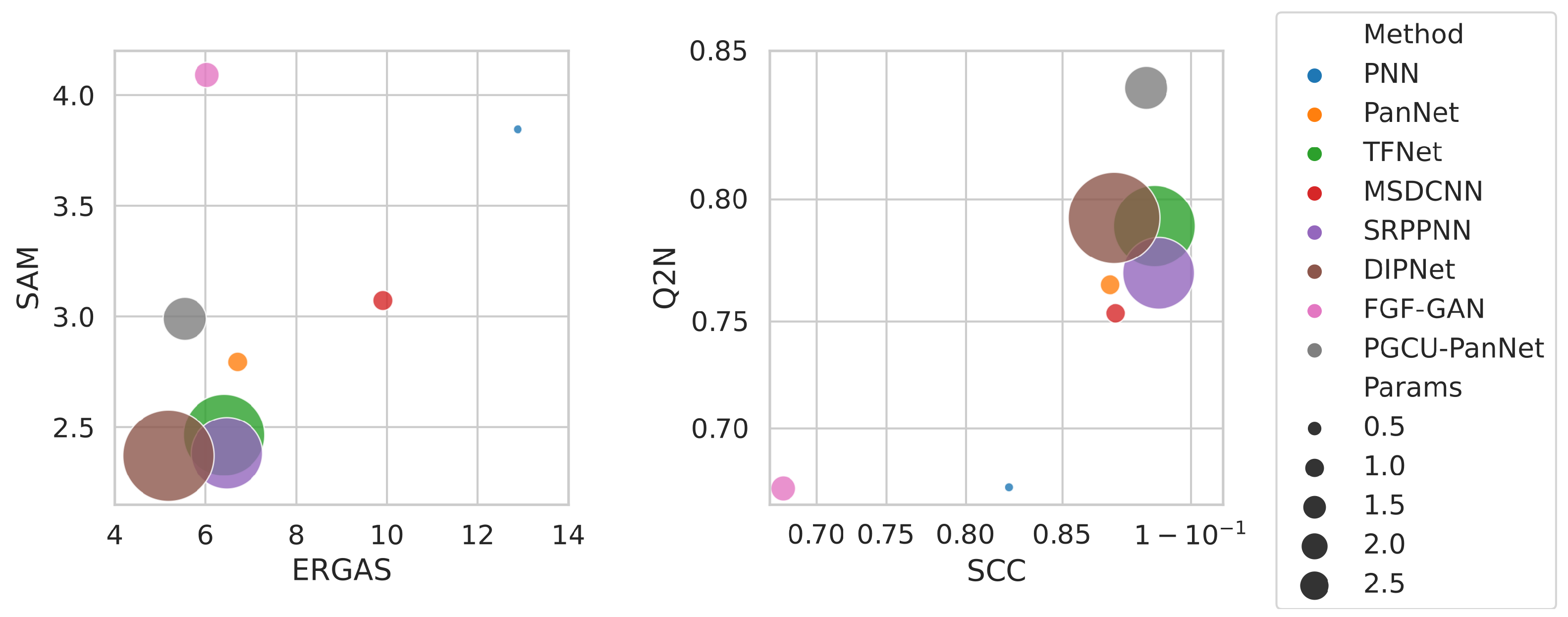
In general, regarding the evaluation with the RR protocol, overall, the most remarkable methods are DIPNet, SRPPNN, and PGCU-PanNet. While DIPNet obtains the best results in terms of the ERGAS and SAM metrics, SRPPNN achieves the best value on SCC, followed by TFNet and PCGU-PanNet. This last model obtained instead the best $Q{2}^n$ followed directly by DIPNet. Overall, even if a different behavior for the different metrics considered is noticeable, DIPNet always achieves good results in this first comparison. The fact that this model obtains the best results in terms of ERGAS and SAM values anticipates the fact that it is probably the best among the considered methods from the spectral fidelity point of view. A more in-depth discussion is provided in Section 4.

Figure 4 reports a graphical comparison between the network-based approaches (in the RR protocol). The comparison evaluates the performance in terms of ERGAS versus SAM (Figure 4, graph on the left) and SCC versus $Q{2}^n$ (Figure 4, graph on the right), along with the number of parameters associated with the neural models. The size of the circles in the figure corresponds to the number of parameters, measured in millions. This information is also reported in Table 4 and Table 5. Larger circles indicate a higher number of parameters. Ideally, the optimal approach would be represented by a small circle positioned in the bottom-left part of Figure 4 left graph and the top-right part of Figure 4 right graph. In practice, the best neural methods are DIPNet, SRPPNN, and TFNet, which have a number of parameters that is about 30 times the number of parameters of lower-performing approaches, such as PanNet and MSDCNN.

The results obtained in the FR protocol are presented in Table 5, revealing a significant shift in the behavior of the models. Notably, TFNet emerges as the top-performing model in terms of $Q^{*}$ index. Surprisingly, DIPNet, which was the winning method in the RR protocol, demonstrates considerably poorer results compared to the other approaches. Even the simpler and smaller PanNet outperforms DIPNet, securing the second position in the comparison.

Analyzing the spatial distortion aspect ($D_s$), the top-performing model is PGCU-PanNet, which obtains the best results with a noticeable gap with respect to the second and third methods, TFNet and MSDCNN. In this case, DIPNet exhibits the weakest performance among the deep learning models. It is worth mentioning that HySure is the best method in terms of $D_s$; however, additional insights regarding its performance can be found in Section 4, where various issues in the spatial reconstruction of this technique are reported.

On the other hand, from a spectral distortion perspective ($D_{\lambda }^k$), PanNet emerges as the best approach, followed by TFNet and DIPNet. A comprehensive qualitative comparison of these two aspects of the reconstruction is presented in the subsequent section. Particularly noteworthy is PanNet’s position in the FR leaderboard, which, considering its comparatively smaller size with respect to other more recent approaches, is notably high in the ranking. The consistency of TFNet is also noticeable, showing the best performance in terms of $Q^{*}$ while achieving the second place for both the $D_{\lambda }$ and $D_s$ metrics.

In conclusion, TFNet emerges as the most successful approach when evaluating with the FR protocol. TFNet exhibits a commendable ability to strike a balance between preserving spectral and spatial information throughout the pansharpening process. When compared to SRPPNN, DIPNet, and PGCU-PanNet, TFNet demonstrates superior generalization capabilities when transitioning from the training resolution of 180 m/px to the native resolution of 30 m/px of the PRISMA satellite HS images.

4. Discussion

With the aim of better understanding the metrics and the results achieved in our analysis, we also propose a qualitative comparison. The objective of this investigation is to illustrate the ability of the analyzed models to preserve the spatial and spectral information after the pansharpening process, without creating distortions. As this study will demonstrate, it is also important to visualize the results of a pansharpening process because an evaluation based on metrics is not always sufficient in terms of indicating the best possible approaches.

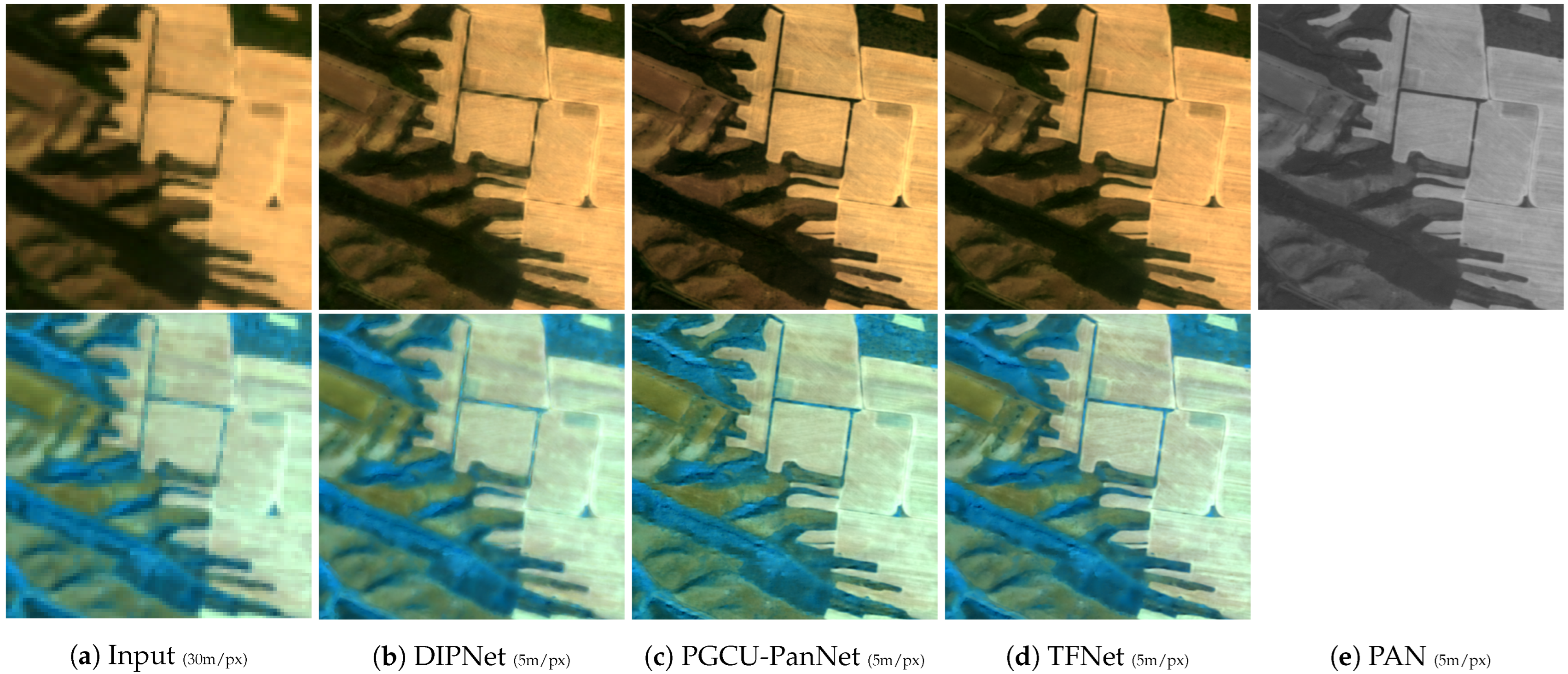
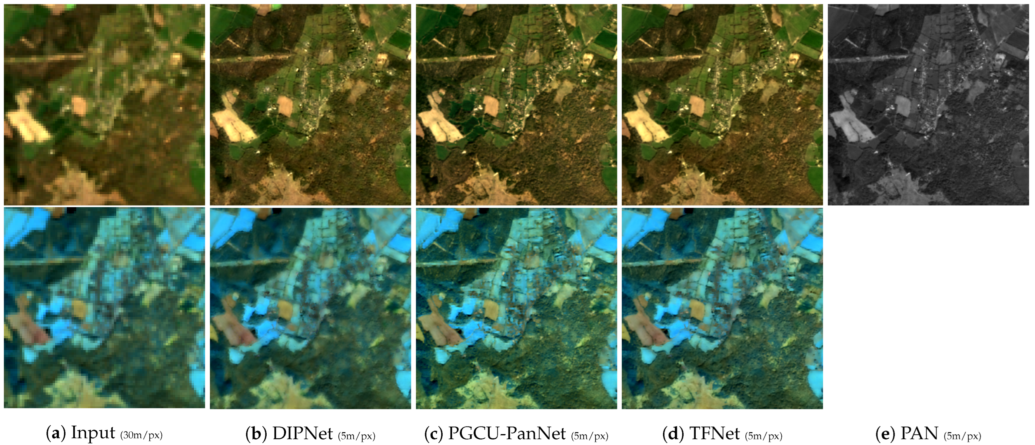
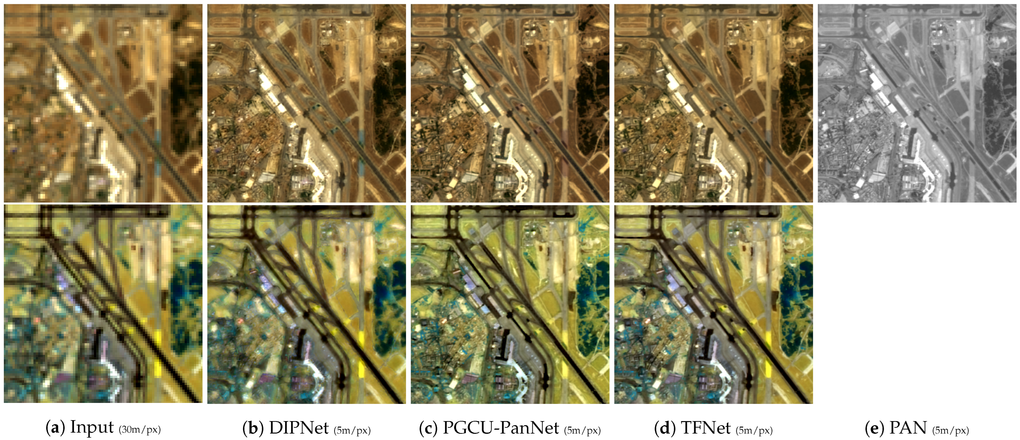
Figure 5, Figure 6 and Figure 7 show the results of the best models on three images of the FR protocol. Here are shown center crops of dimensions $512\times 512$ of the pansharpened images (5 m per pixel) alongside the same crop of the original input image (30 m per pixel). For visualization purposes, the images have been linearly stretched between the 1st and 99th percentile of the image histogram. In the first row, the images are visualized in True Color (641 nm, 563 nm, and 478 nm), and in the second row, the images are in False Color Composite (1586 nm, 1229 nm, and 770 nm). Concerning the spatial information, as can be seen here and as already highlighted by the quantitative comparison, PGCU-PanNet presents the best-looking structures and details overall. Among the considered methods and especially in comparison with DIPNet, TFNet reconstructs much cleaner images, with good edges and a lot more detail. TFNet still achieves good results compared to DIPNet. In Figure 5, Figure 6 and Figure 7, the actual superiority in terms of structure reconstruction obtained by PGCU-PanNet with respect to TFNet, and in particular DIPNet, can be observed. TFNet still achieves sharp results, but still lacks the fine-grained details enhanced by PCGU-PanNet. Overall, DIPNet presents the most blurred results, with a very low number of details and the presence of artifacts, particularly noticeable in the False Color Composite version of the reported scenes.

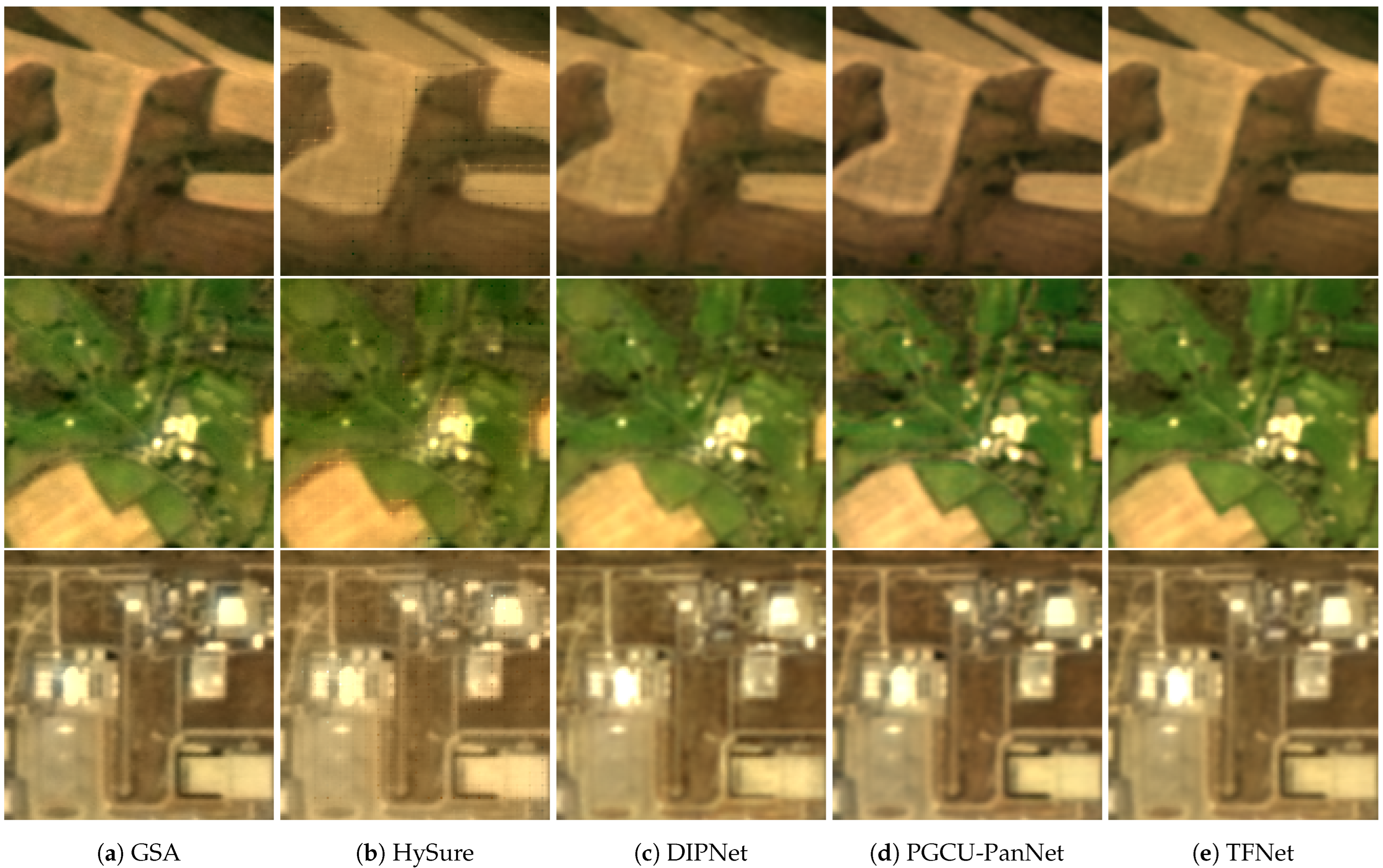
Figure 8 shows zoomed crops at a dimension of $128\times 128$ of areas of the same images processed by the best neural-based and the two best machine-learning-free methods. As can be seen, even if HySure numerically represents the best approach from the spatial point of view (see Table 5, $D_s$ index), a pattern of artifacts occurs over all the images processed by the HySure algorithm. This last comparison shows a potential problem in the adoption of $Q^{*}$ index as a metric for the no-reference analysis, when this type of artifact occurs in the pansharpened images.

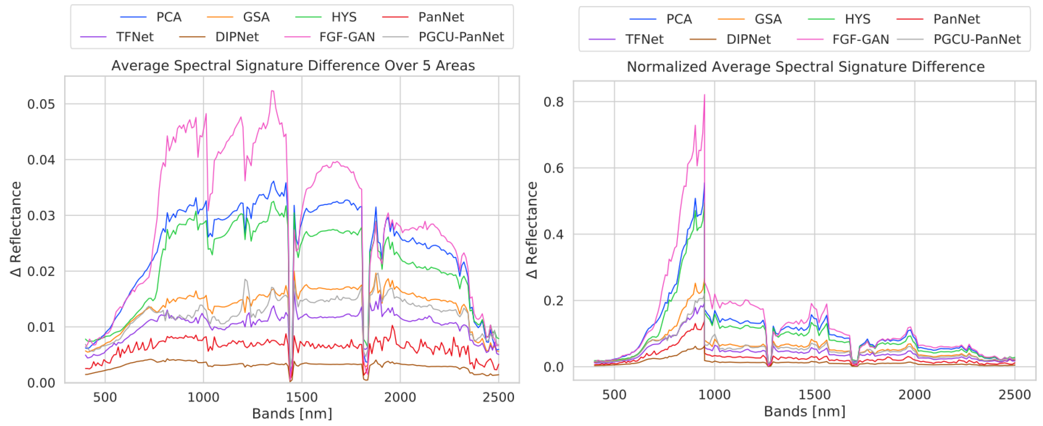
Figure 9 reports the average differences between the spectral signatures of each method and the reference method, alongside the normalized version of the same difference, computed on five different tiles. These tiles have been randomly extracted from the test set. From this comparison, it is possible to notice how DIPNet’s average error is much smaller with respect to the other approaches. Compared with the results from the quantitative evaluation with the FR protocol, where DIPNet reaches third place, this is the only surprising behavior. This unexpected result could provide insight into a possible flaw in the adoption of the spectral component of the $Q^{*}$ metric, as is usually implemented in the literature.

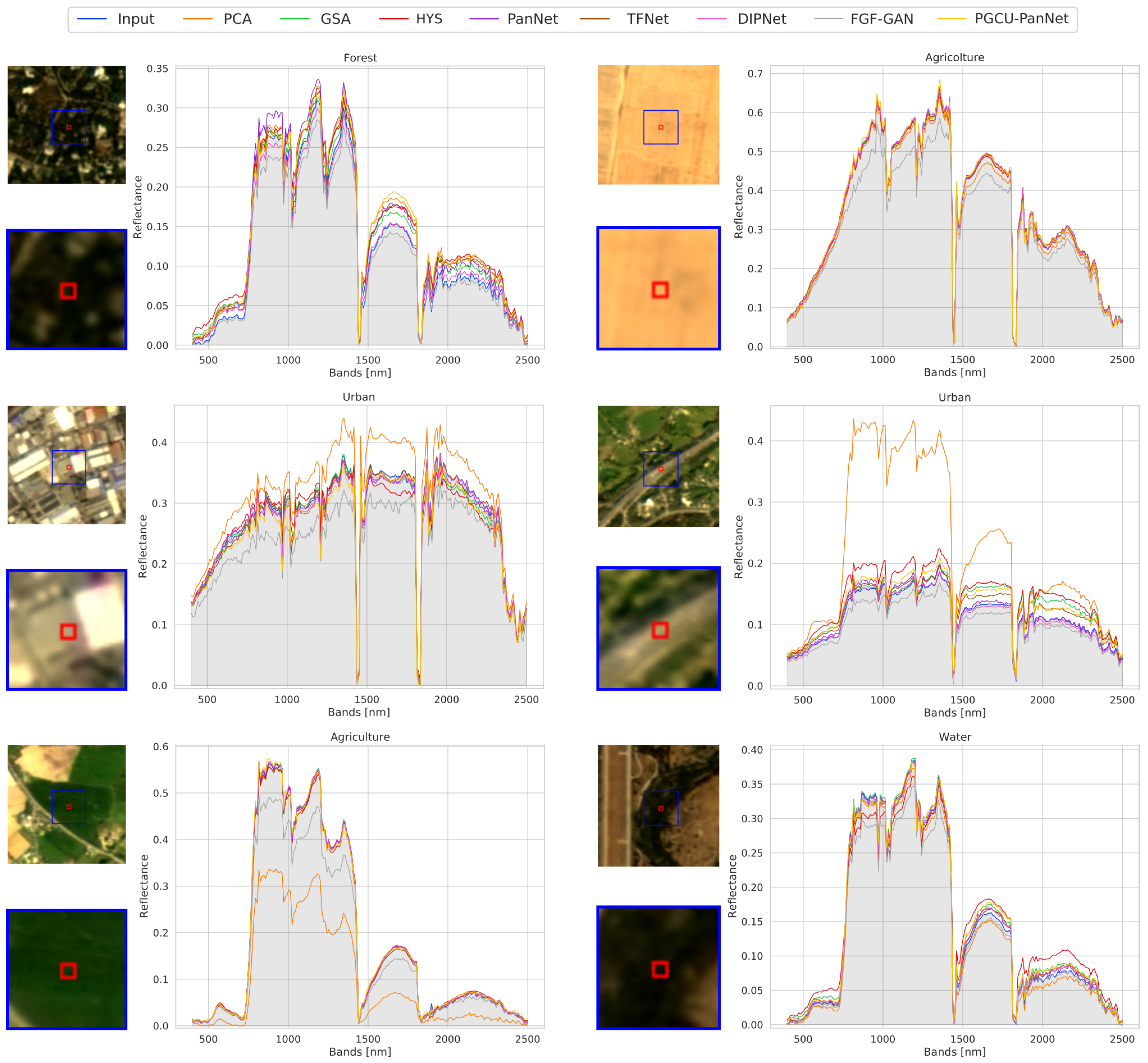
Figure 10 shows the spectral signatures of both input and pansharpened images for each method. Here we have considered only selected groups of pixels, specifically labeled as Forest, Urban, Agriculture, and Water, highlighted in red in the images alongside the graphs. The best method is expected to show signatures closer to the input ones; we have reported both the machine-learning-free and the best deep learning approaches. It is worth noting that all the methods tend to show increased spectral signature differences in the range of 1000 nm to 1500 nm, suggesting this band range is particularly challenging for pansharpening techniques. From this qualitative comparison and in accordance with the numbers in Table 5, PCA, HySure, and FGF-GAN are the worst-performing methods in terms of spectral fidelity. For all the reported classes, these methods perform badly over the entire spectrum with performances worse than GSA. Regarding the deep learning approaches, DIPNet seems to show the lowest difference from the input, despite the score obtained in terms of $D_{\lambda }$ (see Table 5). TFNet and PGCU-PanNet instead have a behavior more coherent with the results obtained in the quantitative evaluation with the FR protocol. It should be noticed that PanNet seems to perform better from a spectral fidelity point of view with respect to TFNet, which, however, performs better than all of the machine-learning-free approaches. Another consideration can be made in relation to the spectral signature difference between PanNet and PGCU-PanNet. The latter method, which is a combination of a specific upsampling module and the original PanNet architecture, achieves much worse results than the actual PanNet. This finding indicates that advances in the MS domain within the visible wavelength spectrum can offer partial benefits in HS applications. Even if, from the FR protocol comparison and in the visual comparison, the model outperforms the others in terms of spatial image enhancement, the spectral reconstruction performs in a poor way with respect to its simpler counterpart.

Overall, we can confirm that the results shown in Table 5, namely DIPNet, PanNet, and TFNet, are the best approaches, with a performance higher in comparison to the machine-learning-free approaches. Based on these three models, the investigation suggests that methods which incorporate structural information into low-resolution images, allowing the network to determine and optimize the feature extraction process from spectral and spatial data, tend to perform better.

Images at a higher resolution are available at https://thezino.github.io/HSbenchmarkPRISMA/, (accessed on 26 May 2024).

5. Conclusions

The increasing availability of HS remote sensing data presents new opportunities for studying the Earth’s soil. However, this type of data is typically collected at a low resolution, posing challenges in terms of their effective usability in RS tasks. Therefore, the process of image pansharpening becomes crucial in the enhancement of HS remote sensing images.

In the literature, deep learning approaches have shown promising results. These methods, however, are data-hungry and state-of-the-art datasets struggle to support sufficient amounts of data. To overcome this limitation, we have proposed a newly collected large-scale dataset using the PRISMA ASI satellite for the training and assessment models.

To the best of our knowledge, this work is the first to present an analysis based on a large and varied HS dataset for pansharpening in the state of the art (consisting of more than 1000 tiles, of which more than 200 have been used for the testing). The dataset tiles have been collected from 190 PRISMA images with 203 bands, (The original number of PRISMA spectral bands is 240. The number reported above was obtained after the proposed pre-processing procedure.) covering both the VNIR and SWIR parts of the spectrum, making this investigation the optimal benchmark for hyperspectral pansharpening.

The comparison includes machine-learning-free and deep learning techniques tested using two experimental protocols for a $6\times$ upscaling factor: RR and FR. The former is used for training and testing, and the latter to test the methods on the original resolution, evaluating their ability to generalize the upsampling operation at different starting resolutions with respect to the training phase.

The RR protocol consists of a comparison between the reconstructed data and the original HS images as target references. The results show that the neural networks generally work better than the machine-learning-free methods in terms of spatial information improvement and spectral information coherency. In particular, DIPNet and TFNet architectures outperform all the other techniques evaluated. In the FR protocol, the comparison with ground truths has not been possible, and therefore, quantitative and also qualitative evaluations have been reported to provide a complete understanding of the methods investigated. Based on both assessments, the architecture that achieves the best overall performance is TFNet, which remains coherent with the RR results. PanNet proves to be a good alternative mainly on account of its capability of spectral reconstruction and its limited number of parameters, which makes it the best option in the case of environments with computational resource constraints. Finally, DIPNet shows worse results when it comes to spatial reconstruction, not demonstrating good abilities of adaptation when the original resolution is involved and thus not being the best option for tests in real-world applications. However, from the qualitative investigation, it seems to be the one that causes less spectral distortion, remaining a valid option for tasks where spectral fidelity is particularly important. It is also worth noticing that machine-learning-free methods are generally worse at reconstructing the spectral information, degrading the signals.

The investigation conducted in this work clearly shows that data-driven neural architectures are generally better for HS pansharpening, in terms of both spectral and spatial reconstruction, using a dataset that allows for meaningful analysis of the different approaches. On the contrary, the machine-learning-free methods are not adaptable to the new environment based on HS data and wavelengths outside the visible part of the spectrum.

HS data give us the best spectral information possible and are used in many different tasks, from semantic segmentation to unmixing. In remote sensing, the problem of low spatial resolution affects all of these tasks and needs to be addressed with algorithms specifically designed for these kinds of data. In our opinion, to further improve our understanding of and ability to perform HS pansharpening, the availability of statistically relevant datasets for testing and training can lead to future improvements not only in the field of pansharpening but also in all those tasks that consider pansharpening as a fundamental step in their pipelines. Starting from this analysis, new HS methods should be developed based on an evaluation of the relationship between the different portions of the spectrum and the spatial information from the panchromatic data. Another interesting direction could be the integration of this knowledge with the recent generative models and their ability to reconstruct new and lost information could significantly improve the performance of pansharpening techniques and consequently other tasks.

References

1. Salcedo-Sanz, S.; Ghamisi, P.; Piles, M.; Werner, M.; Cuadra, L.; Moreno-Martínez, A.; Izquierdo-Verdiguier, E.; Muñoz-Marí, J.; Mosavi, A.; Camps-Valls, G. Machine learning information fusion in Earth observation: A comprehensive review of methods, applications and data sources. Inf. Fusion 2020, 63, 256–272. [Google Scholar] [CrossRef]
2. Barbato, M.P.; Napoletano, P.; Piccoli, F.; Schettini, R. Unsupervised segmentation of hyperspectral remote sensing images with superpixels. Remote Sens. Appl. Soc. Environ. 2022, 28, 100823. [Google Scholar] [CrossRef]
3. Iglseder, A.; Immitzer, M.; Dostálová, A.; Kasper, A.; Pfeifer, N.; Bauerhansl, C.; Schöttl, S.; Hollaus, M. The potential of combining satellite and airborne remote sensing data for habitat classification and monitoring in forest landscapes. Int. J. Appl. Earth Obs. Geoinf. 2023, 117, 103131. [Google Scholar] [CrossRef]
4. Sishodia, R.P.; Ray, R.L.; Singh, S.K. Applications of remote sensing in precision agriculture: A review. Remote Sens. 2020, 12, 3136. [Google Scholar] [CrossRef]
5. Wellmann, T.; Lausch, A.; Andersson, E.; Knapp, S.; Cortinovis, C.; Jache, J.; Scheuer, S.; Kremer, P.; Mascarenhas, A.; Kraemer, R.; et al. Remote sensing in urban planning: Contributions towards ecologically sound policies? Landsc. Urban Plan. 2020, 204, 103921. [Google Scholar] [CrossRef]
6. Van Westen, C. Remote sensing for natural disaster management. Int. Arch. Photogramm. Remote Sens. 2000, 33, 1609–1617. [Google Scholar]
7. Frick, A.; Tervooren, S. A framework for the long-term monitoring of urban green volume based on multi-temporal and multi-sensoral remote sensing data. J. Geovis. Spat. Anal. 2019, 3, 6. [Google Scholar] [CrossRef]
8. Costs, S.T. Trends in Price per Pound to Orbit 1990–2000; Futron Corporation: Bethesda, MD, USA, 2002. [Google Scholar]
9. Jones, H. The recent large reduction in space launch cost. In Proceedings of the 48th International Conference on Environmental Systems, Albuquerque, NM, USA, 8–12 July 2018. [Google Scholar]
10. Okninski, A.; Kopacz, W.; Kaniewski, D.; Sobczak, K. Hybrid rocket propulsion technology for space transportation revisited-propellant solutions and challenges. FirePhysChem 2021, 1, 260–271. [Google Scholar] [CrossRef]
11. Wulder, M.A.; Loveland, T.R.; Roy, D.P.; Crawford, C.J.; Masek, J.G.; Woodcock, C.E.; Allen, R.G.; Anderson, M.C.; Belward, A.S.; Cohen, W.B.; et al. Current status of Landsat program, science, and applications. Remote Sens. Environ. 2019, 225, 127–147. [Google Scholar] [CrossRef]
12. Chevrel, M.; Courtois, M.; Weill, G. The SPOT satellite remote sensing mission. Photogramm. Eng. Remote Sens. 1981, 47, 1163–1171. [Google Scholar]
13. Phiri, D.; Simwanda, M.; Salekin, S.; Nyirenda, V.R.; Murayama, Y.; Ranagalage, M. Sentinel-2 data for land cover/use mapping: A review. Remote Sens. 2020, 12, 2291. [Google Scholar] [CrossRef]
14. Apostolopoulos, D.N.; Nikolakopoulos, K.G. SPOT vs. Landsat satellite images for the evolution of the north Peloponnese coastline, Greece. Reg. Stud. Mar. Sci. 2022, 56, 102691. [Google Scholar] [CrossRef]
15. Krueger, J.K. CLOSeSat: Perigee-Lowering Techniques and Preliminary Design for a Small Optical Imaging Satellite Operating in Very Low Earth Orbit. Ph.D. Thesis, Massachusetts Institute of Technology, Cambridge, MA, USA, 2010. [Google Scholar]
16. Li, S.; Kang, X.; Fang, L.; Hu, J.; Yin, H. Pixel-level image fusion: A survey of the state of the art. Inf. Fusion 2017, 33, 100–112. [Google Scholar] [CrossRef]
17. Vivone, G.; Alparone, L.; Chanussot, J.; Dalla Mura, M.; Garzelli, A.; Licciardi, G.A.; Restaino, R.; Wald, L. A critical comparison among pansharpening algorithms. IEEE Trans. Geosci. Remote Sens. 2014, 53, 2565–2586. [Google Scholar] [CrossRef]
18. Loncan, L.; De Almeida, L.B.; Bioucas-Dias, J.M.; Briottet, X.; Chanussot, J.; Dobigeon, N.; Fabre, S.; Liao, W.; Licciardi, G.A.; Simoes, M.; et al. Hyperspectral pansharpening: A review. IEEE Geosci. Remote Sens. Mag. 2015, 3, 27–46. [Google Scholar] [CrossRef]
19. Chavez, P.; Sides, S.C.; Anderson, J.A. Comparison of three different methods to merge multiresolution and multispectral data- Landsat TM and SPOT panchromatic. Photogramm. Eng. Remote Sens. 1991, 57, 295–303. [Google Scholar]
20. Tu, T.M.; Huang, P.S.; Hung, C.L.; Chang, C.P. A fast intensity-hue-saturation fusion technique with spectral adjustment for IKONOS imagery. IEEE Geosci. Remote Sens. Lett. 2004, 1, 309–312. [Google Scholar] [CrossRef]
21. Laben, C.A.; Brower, B.V. Process for Enhancing the Spatial Resolution of Multispectral Imagery Using Pan-Sharpening. U.S. Patent 6,011,875, 4 January 2000. [Google Scholar]
22. Aiazzi, B.; Baronti, S.; Selva, M. Improving Component Substitution Pansharpening Through Multivariate Regression of MS +Pan Data. IEEE Trans. Geosci. Remote Sens. 2007, 45, 3230–3239. [Google Scholar] [CrossRef]
23. Mallat, S.G. A theory for multiresolution signal decomposition: The wavelet representation. IEEE Trans. Pattern Anal. Mach. Intell. 1989, 11, 674–693. [Google Scholar] [CrossRef]
24. Nason, G.P.; Silverman, B.W. The stationary wavelet transform and some statistical applications. In Wavelets and Statistics; Springer: New York, NY, USA, 1995; pp. 281–299. [Google Scholar]
25. Shensa, M.J. The discrete wavelet transform: Wedding the a trous and Mallat algorithms. IEEE Trans. Signal Process. 1992, 40, 2464–2482. [Google Scholar] [CrossRef]
26. Burt, P.J.; Adelson, E.H. The Laplacian pyramid as a compact image code. In Readings in Computer Vision; Elsevier: Amsterdam, The Netherlands, 1987; pp. 671–679. [Google Scholar]
27. Liao, W.; Huang, X.; Van Coillie, F.; Gautama, S.; Pižurica, A.; Philips, W.; Liu, H.; Zhu, T.; Shimoni, M.; Moser, G.; et al. Processing of multiresolution thermal hyperspectral and digital color data: Outcome of the 2014 IEEE GRSS data fusion contest. IEEE J. Sel. Top. Appl. Earth Obs. Remote Sens. 2015, 8, 2984–2996. [Google Scholar] [CrossRef]
28. Zhang, K.; Zhang, F.; Wan, W.; Yu, H.; Sun, J.; Del Ser, J.; Elyan, E.; Hussain, A. Panchromatic and multispectral image fusion for remote sensing and earth observation: Concepts, taxonomy, literature review, evaluation methodologies and challenges ahead. Inf. Fusion 2023, 93, 227–242. [Google Scholar] [CrossRef]
29. He, L.; Zhu, J.; Li, J.; Plaza, A.; Chanussot, J.; Li, B. HyperPNN: Hyperspectral pansharpening via spectrally predictive convolutional neural networks. IEEE J. Sel. Top. Appl. Earth Obs. Remote Sens. 2019, 12, 3092–3100. [Google Scholar] [CrossRef]
30. He, L.; Zhu, J.; Li, J.; Meng, D.; Chanussot, J.; Plaza, A. Spectral-fidelity convolutional neural networks for hyperspectral pansharpening. IEEE J. Sel. Top. Appl. Earth Obs. Remote Sens. 2020, 13, 5898–5914. [Google Scholar] [CrossRef]
31. Zheng, Y.; Li, J.; Li, Y.; Cao, K.; Wang, K. Deep residual learning for boosting the accuracy of hyperspectral pansharpening. IEEE Geosci. Remote Sens. Lett. 2019, 17, 1435–1439. [Google Scholar] [CrossRef]
32. Xie, W.; Lei, J.; Cui, Y.; Li, Y.; Du, Q. Hyperspectral pansharpening with deep priors. IEEE Trans. Neural Netw. Learn. Syst. 2019, 31, 1529–1543. [Google Scholar] [CrossRef]
33. He, L.; Xi, D.; Li, J.; Lai, H.; Plaza, A.; Chanussot, J. Dynamic hyperspectral pansharpening CNNs. IEEE Trans. Geosci. Remote Sens. 2023, 61, 1–19. [Google Scholar] [CrossRef]
34. Zhao, Z.; Zhan, J.; Xu, S.; Sun, K.; Huang, L.; Liu, J.; Zhang, C. FGF-GAN: A lightweight generative adversarial network for pansharpening via fast guided filter. In Proceedings of the 2021 IEEE International Conference on Multimedia and Expo (ICME), Shenzhen, China, 5–9 July 2021; pp. 1–6. [Google Scholar]
35. He, K.; Sun, J. Fast guided filter. arXiv 2015, arXiv:1505.00996. [Google Scholar]
36. Zhu, Z.; Cao, X.; Zhou, M.; Huang, J.; Meng, D. Probability-based global cross-modal upsampling for pansharpening. In Proceedings of the IEEE/CVF Conference on Computer Vision and Pattern Recognition, Vancouver, BC, Canada, 17–24 June 2023; pp. 14039–14048. [Google Scholar]
37. Vivone, G.; Garzelli, A.; Xu, Y.; Liao, W.; Chanussot, J. Panchromatic and hyperspectral image fusion: Outcome of the 2022 whispers hyperspectral pansharpening challenge. IEEE J. Sel. Top. Appl. Earth Obs. Remote Sens. 2022, 16, 166–179. [Google Scholar] [CrossRef]
38. Labate, D.; Safari, K.; Karantzas, N.; Prasad, S.; Shahraki, F.F. Structured receptive field networks and applications to hyperspectral image classification. In Proceedings of the Wavelets and Sparsity XVIII, San Diego, CA, USA, 13–15 August 2019; SPIE: Bellingham, WA, USA, 2019; Volume 11138, pp. 218–226. [Google Scholar]
39. Yokoya, N.; Iwasaki, A. Airborne Hyperspectral Data over Chikusei; Report Number: SAL-2016-5-27; Space Application Laboratory, University of Tokyo: Tokyo, Japan, 2016; Volume 5. [Google Scholar]
40. Baumgardner, M.F.; Biehl, L.L.; Landgrebe, D.A. 220 Band Aviris Hyperspectral Image Data Set: June 12, 1992 Indian Pine Test Site 3; Purdue University Research Repository: West Lafayette, IN, USA, 2015; Volume 10, p. 991. [Google Scholar]
41. ASI. PRISMA Algorithm Theoretical Basis Document (ATBD). 2021. Available online: https://prisma.asi.it/missionselect/docs/PRISMA%20ATBD_v1.pdf (accessed on 3 April 2023).
42. Potapov, P.; Hansen, M.C.; Pickens, A.; Hernandez-Serna, A.; Tyukavina, A.; Turubanova, S.; Zalles, V.; Li, X.; Khan, A.; Stolle, F.; et al. The global 2000–2020 land cover and land use change dataset derived from the Landsat archive: First results. Front. Remote Sens. 2022, 3, 856903. [Google Scholar] [CrossRef]
43. Scheffler, D.; Hollstein, A.; Diedrich, H.; Segl, K.; Hostert, P. AROSICS: An automated and robust open-source image co-registration software for multi-sensor satellite data. Remote Sens. 2017, 9, 676. [Google Scholar] [CrossRef]
44. Wald, L. Data Fusion: Definitions and Architectures: Fusion of Images of Different Spatial Resolutions; Presses des MINES: Paris, France, 2002. [Google Scholar]
45. Yuhas, R.H.; Goetz, A.F.; Boardman, J.W. Discrimination among semi-arid landscape endmembers using the spectral angle mapper (SAM) algorithm. In Proceedings of the JPL, Summaries of the Third Annual JPL Airborne Geoscience Workshop, Volume 1: AVIRIS Workshop, Pasadena, CA, USA, 1–5 June 1992. [Google Scholar]
46. Zhou, J.; Civco, D.L.; Silander, J.A. A wavelet transform method to merge Landsat TM and SPOT panchromatic data. Int. J. Remote Sens. 1998, 19, 743–757. [Google Scholar] [CrossRef]
47. Wang, Z.; Bovik, A.C. A universal image quality index. IEEE Signal Process. Lett. 2002, 9, 81–84. [Google Scholar] [CrossRef]
48. Arienzo, A.; Vivone, G.; Garzelli, A.; Alparone, L.; Chanussot, J. Full-resolution quality assessment of pansharpening: Theoretical and hands-on approaches. IEEE Geosci. Remote Sens. Mag. 2022, 10, 168–201. [Google Scholar] [CrossRef]
49. Wald, L.; Ranchin, T.; Mangolini, M. Fusion of satellite images of different spatial resolutions: Assessing the quality of resulting images. Photogramm. Eng. Remote Sens. 1997, 63, 691–699. [Google Scholar]
50. Alparone, L.; Garzelli, A.; Vivone, G. Spatial consistency for full-scale assessment of pansharpening. In Proceedings of the IGARSS 2018—2018 IEEE International Geoscience and Remote Sensing Symposium, Valencia, Spain, 22–27 July 2018; pp. 5132–5134. [Google Scholar]
51. Simoes, M.; Bioucas-Dias, J.; Almeida, L.B.; Chanussot, J. A convex formulation for hyperspectral image superresolution via subspace-based regularization. IEEE Trans. Geosci. Remote Sens. 2014, 53, 3373–3388. [Google Scholar] [CrossRef]
52. Masi, G.; Cozzolino, D.; Verdoliva, L.; Scarpa, G. Pansharpening by convolutional neural networks. Remote Sens. 2016, 8, 594. [Google Scholar] [CrossRef]
53. Yang, J.; Fu, X.; Hu, Y.; Huang, Y.; Ding, X.; Paisley, J. PanNet: A deep network architecture for pan-sharpening. In Proceedings of the IEEE International Conference on Computer Vision, Piscataway, NJ, USA, 22–29 October 2017; pp. 5449–5457. [Google Scholar]
54. Yuan, Q.; Wei, Y.; Meng, X.; Shen, H.; Zhang, L. A multiscale and multidepth convolutional neural network for remote sensing imagery pan-sharpening. IEEE J. Sel. Top. Appl. Earth Obs. Remote Sens. 2018, 11, 978–989. [Google Scholar] [CrossRef]
55. Liu, X.; Liu, Q.; Wang, Y. Remote sensing image fusion based on two-stream fusion network. Inf. Fusion 2020, 55, 1–15. [Google Scholar] [CrossRef]
56. Cai, J.; Huang, B. Super-resolution-guided progressive pansharpening based on a deep convolutional neural network. IEEE Trans. Geosci. Remote Sens. 2020, 59, 5206–5220. [Google Scholar] [CrossRef]
57. Xie, Y.; Wu, W.; Yang, H.; Wu, N.; Shen, Y. Detail information prior net for remote sensing image pansharpening. Remote Sens. 2021, 13, 2800. [Google Scholar] [CrossRef]
Figure 1. Map of the patches acquired using the PRISMA satellite. On average, each patch covers about 1380 km2 of soil. Each red box corresponds to a land-patch.
Remotesensing 16 02079 g001
Figure 2. Examples of PRISMA dataset entries, visualized in True Color RGB (641 nm, 563 nm, 478 nm). The P A N image is at a resolution of 5 m per pixel, the H S images are at 30 m per pixel, and the H S are at 180 m per pixel.
Remotesensing 16 02079 g002
Figure 3. Distribution of the invalid bands for each PRISMA image collected. In (a), the scale indicates the percentage of invalid pixels for each band of each image collected from the PRISMA satellite. Bands that are considered invalid for at least one image (with more than 5% of the entries invalid) were selected for removal. In (b), the average spectral signatures per image and the bands excluded in the final version of the dataset are shown.
Remotesensing 16 02079 g003
Figure 4. Graph comparison of the results of the analyzed methods with the RR protocol. The larger the size of the circle, the higher the number of parameters (measured in millions).
Remotesensing 16 02079 g004
Figure 5. Pansharpening results on a 512 × 512 tile of a test set image. For visualization purposes, the images have been linearly stretched between the 1st and 99th percentile of the image histogram. In the first row, images are visualized in True Color (641 nm, 563 nm, and 478 nm), and in the second row, the images are in False Color Composite (1586 nm, 1229 nm, and 770 nm).
Remotesensing 16 02079 g005
Figure 6. Pansharpening results on a 512 × 512 tile of a test set image. For visualization purposes, the images have been linearly stretched between the 1st and 99th percentile of the image histogram. In the first row, images are visualized in True Color (641 nm, 563 nm, and 478 nm), and in the second row, the images are in False Color Composite (1586 nm, 1229 nm, and 770 nm).
Remotesensing 16 02079 g006
Figure 7. Pansharpening results on a 512 × 512 tile of a test set image. For visualization purposes, the images have been linearly stretched between the 1st and 99th percentile of the image histogram. In the first row, the images are visualized in True Color (641 nm, 563 nm, and 478 nm), and in the second row, the images are in False Color Composite (1586 nm, 1229 nm, and 770 nm).
Remotesensing 16 02079 g007
Figure 8. Zoom of areas from the test images. Crops of dimension 128 × 128 , at a resolution of 5 m/px, in True Color (641 nm, 563 nm, and 478 nm). As can be seen, repeated artifacts along the edges can be observed for the HySure method.
Remotesensing 16 02079 g008
Figure 9. Differences between the spectral signatures of the fused images with respect to the input image. The difference is evaluated as the average of the differences for each pixel of the five images reported in the row below the graph. The graph on the left shows the average spectral difference, while the graph on the right shows the difference normalized for each band.
Remotesensing 16 02079 g009aRemotesensing 16 02079 g009b
Figure 10. Spectral signatures obtained in six different areas, labeled as Forest, Urban, Agriculture, and Water areas. For each area, the spectral signatures of the input bands and those obtained by each pansharpening method are presented. The area used to extract the signatures is the one in the red box highlighted in each image. The image thumbnails are in True Color (641 nm, 563 nm, and 478 nm).
Remotesensing 16 02079 g010