Article

U-Net Ensemble for Enhanced Semantic Segmentation in Remote Sensing Imagery

Faculty of Computer Science and Engineering, University Ss Cyril and Methodius, 1000 Skopje, North Macedonia
*
Author to whom correspondence should be addressed.
Remote Sens. 2024, 16(12), 2077; https://doi.org/10.3390/rs16122077
Submission received: 5 April 2024 / Revised: 31 May 2024 / Accepted: 4 June 2024 / Published: 8 June 2024
(This article belongs to the Special Issue GeoAI and EO Big Data Driven Advances in Earth Environmental Science)

Abstract

:
Semantic segmentation of remote sensing imagery stands as a fundamental task within the domains of both remote sensing and computer vision. Its objective is to generate a comprehensive pixel-wise segmentation map of an image, assigning a specific label to each pixel. This facilitates in-depth analysis and comprehension of the Earth’s surface. In this paper, we propose an approach for enhancing semantic segmentation performance by employing an ensemble of U-Net models with three different backbone networks: Multi-Axis Vision Transformer, ConvFormer, and EfficientNet. The final segmentation maps are generated through a geometric mean ensemble method, leveraging the diverse representations learned by each backbone network. The effectiveness of the base U-Net models and the proposed ensemble is evaluated on multiple datasets commonly used for semantic segmentation tasks in remote sensing imagery, including LandCover.ai, LoveDA, INRIA, UAVid, and ISPRS Potsdam datasets. Our experimental results demonstrate that the proposed approach achieves state-of-the-art performance, showcasing its effectiveness and robustness in accurately capturing the semantic information embedded within remote sensing images.

1. Introduction

Remote sensing images encompass imagery captured from a distance by sensors or instruments mounted on various platforms such as satellites, aircraft, drones, and other vehicles. These images serve to gather information about the Earth’s surface, atmosphere, and other objects or phenomena without requiring direct physical contact [1]. There are two main types of remote sensing images: aerial and satellite. Both aerial and satellite images are valuable sources of data, but they differ in how they collect data and their characteristics [2]. Satellites travel around Earth, collecting data from large areas at regular intervals. This provides a broad view of the entire planet. Aerial images are captured from airplanes or drones flying closer to the ground. They cover smaller areas but with much finer detail, making them ideal for studying specific locations. The choice between aerial and satellite imagery depends on the specific needs of the application at hand, such as the level of detail required and the availability of data [3].
The recent surge in sophisticated machine learning techniques, coupled with the ever-growing availability of remote sensing data, has significantly empowered image analysis and interpretation [4,5,6,7]. Semantic segmentation, a technique that assigns a specific class/annotation/label to each pixel in an image, has become a major research focus for remote sensing imagery [3]. This approach allows for a highly detailed analysis of ground objects and their spatial relationships. Unlike object detection, which focuses on identifying and roughly locating objects, semantic segmentation provides fine-grained pixel-level identification, enabling a deeper understanding of the image’s content [8,9,10]. Semantic segmentation in remote sensing has far-reaching implications across various domains, such as urban planning [11,12,13], disaster management [14,15,16], environmental monitoring, and precision agriculture [17,18,19,20].
The emergence of deep learning, particularly convolutional neural networks (CNNs) and fully convolutional networks (FCNs), revolutionized the field of semantic segmentation by enabling the automatic learning of hierarchical representations from data [21]. Methods based on FCNs in combination with encoder–decoder architectures have become the dominant approach for semantic segmentation. Early methods utilized a series of successive convolutions followed by spatial pooling to achieve dense predictions [22]. Subsequent approaches, for example, U-Net [23] and SegNet [24], employed upsampling of high-level feature maps combined with low-level ones during decoding, aiming to capture global context and restore precise object boundaries. To enhance the receptive field of convolutions in initial layers, various techniques such as DeepLab [25] introduced dilated or atrous convolutions. Subsequent advancements integrated spatial pyramid pooling to capture multiscale contextual details in higher layers, as seen in models like PSPNet [26] and UperNet [27]. Incorporating these advancements, including atrous spatial pyramid pooling, DeepLabV3+ introduced a straightforward yet efficient encoder–decoder FCN architecture [28]. Subsequent developments, such as those seen in PSANet [29] and DRANet [30], replaced traditional pooling with attention mechanisms atop encoder feature maps to better grasp long-range dependencies.
Most recently, the adoption of transformer architectures, which utilize self-attention mechanisms and capture long-range dependencies, has marked additional advancement in semantic segmentation [31]. Transformer encoder–decoder architectures like Segmenter [32], SegFormer [33], and MaskFormer [34] harness transformers to enhance performance. Segmenter, a transformer encoder–decoder architecture designed for semantic image segmentation, utilizes a vision transformer (ViT) backbone and incorporates a mask decoder. SegFormer is a semantic segmentation framework that combines mix transformer encoders with lightweight multilayer perceptron (MLP) decoders, offering a simple, efficient, yet powerful solution. MaskFormer is a versatile semantic segmentation architecture inspired by DEtection TRansformer (DETR) [35]. It employs a transformer decoder to generate masks for individual objects in an image, utilizing a single decoder for various segmentation tasks. In response to the constraints of MaskFormer, Mask2Former was developed, featuring a multiscale decoder and a masked attention mechanism [36].
Despite the advancements in deep learning and semantic segmentation techniques, accurately segmenting remote sensing images remains a challenging task due to factors like complex spatial structures, diverse object sizes, data imbalance, and high background complexity [3]. Remote sensing images can have a wide range of resolutions and object orientations, posing challenges for consistent segmentation. Objects within a single image can vary dramatically in size. Buildings might stand tall next to tiny patches of vegetation. Effective models need to handle this wide spectrum of scales and accurately segment objects regardless of their relative size. Densely packed objects (like urban buildings) or very small objects (like individual trees) can be difficult for models to identify and segment accurately. Certain classes within a remote sensing image might be under-represented compared to others. For example, rare land cover types might have far fewer pixels compared to common vegetation classes. This data imbalance can make it difficult for models to learn accurate representations of all classes and lead to biased segmentation results. The foreground (objects of interest) might occupy a much smaller area compared to the background, making segmentation lopsided. Moreover, backgrounds in aerial images can be intricate and cluttered (e.g., urban environments), further complicating object segmentation [37].
In the context of semantic segmentation of remote sensing images, several approaches were proposed to overcome these challenges [38,39,40]. AerialFormer utilizes a hierarchical structure, in which a transformer encoder generates multiscale features, while a multidilated convolutional neural network (MD-CNN) decoder aggregates information from these diverse inputs [38]. The UNetFormer model incorporates a global–local transformer block (GLTB) within its decoder to construct the output [39]. Additionally, it utilizes a feature refinement head (FRH) for optimizing the extracted global–local context. For efficiency, the transformer decoder is combined with a lightweight CNN-based encoder. Uncertainty-Aware Network (UANet) introduces the concept of uncertainty and proposes a novel network that leverages this concept [40]. UANet improves the accuracy of distinguishing building footprints from the complex distribution of surrounding ground objects. These advancements demonstrate the ongoing efforts to improve the semantic segmentation of remote sensing images through innovative deep learning architectures.
This paper examines the impact of incorporating powerful backbones into the U-Net architecture to potentially improve the semantic segmentation of remote sensing imagery. We leverage three such backbone networks: Multi-Axis Vision Transformer (MaxViT), ConvFormer, and EfficientNet. MaxViT is a hybrid vision transformer architecture, ConvFormer utilizes convolutional layers within a transformer framework, and EfficientNet is a CNN architecture known for its balance between accuracy and computational cost. We further enhance the performance by employing an ensemble learning approach. The diverse backbones within the ensemble extract complementary features from the images, leading to a richer and more comprehensive understanding of the scene. The ensemble benefits from the unique representations learned by each backbone within the U-Net architecture, leading to more robust and accurate segmentation results. To combine the base predictions, we employ a geometric mean ensemble strategy. To this end, we investigate the potential of combining backbones with different strengths to improve U-Net’s performance for remote sensing semantic segmentation tasks. By exploiting the diversity and utilizing a geometric mean ensemble strategy, we managed to achieve state-of-the-art performance over several semantic segmentation datasets for remote sensing imagery. Our research can be summarized by the following primary contributions:
  • Integration of three strong backbone networks within U-Net: the Multi-Axis Vision Transformer (MaxViT), ConvFormer, and EfficientNet. These models exhibit exceptionally high performance, surpassing previous models with similar model sizes.
  • Introduction of an ensemble learning approach that leverages the complementary strengths of each backbone, tailored to enhance semantic segmentation of remote sensing imagery. Limiting the ensemble to three base models provides a good balance between performance gains and computational cost.
  • Conducting of a comprehensive comparison of our approach with existing methods on various remote sensing image datasets. The experimental results show the superior performance of our models. Visual results further validate the effectiveness of our approach by showcasing accurate segmentation maps in remote sensing images.
The subsequent sections of this paper are organized as follows: In Section 2, we introduce the evaluation datasets, outlining their main characteristics and preprocessing steps. This section also provides insights into the selected backbones and how they are integrated into the ensemble. Additionally, Section 2 elaborates on the experimental setup employed for conducting the experiments. Moving on to Section 3, we present and summarize the obtained results, with detailed analyses and discussions provided. Finally, Section 4 offers concluding remarks.

2. Materials and Methods

2.1. Data Description

Remote sensing has become a powerful tool for analyzing and understanding the Earth’s surface. Semantic segmentation datasets play a crucial role in this field, providing high-resolution satellite and aerial imagery alongside detailed pixel-level annotations [41]. By leveraging these datasets, researchers can train machine learning models to automatically extract meaningful information from vast amounts of remote sensing imagery. In our experimental study, we consider five datasets for semantic segmentation of remote sensing images: LoveDA [42], LandCover.ai [12], UAVid [43], INRIA [11], and ISPRS Potsdam, https://www.isprs.org/education/benchmarks/UrbanSemLab/semantic-labeling.aspx (accessed on 5 June 2024). These datasets present a diverse landscape, with variations in the amount of imagery, types of scenes captured, image resolution, and file formats. This diversity can be both an advantage and a challenge for researchers.
The LoveDA (Land-cOVEr Domain Adaptive) semantic segmentation dataset, https://github.com/Junjue-Wang/LoveDA (accessed on 5 June 2024), consists of 5987 high-resolution images sourced from Google Earth at 0.3 m spatial resolution and a pixel resolution of 1024 × 1024 divided into training, validation, and test sets by the creators [42]. Each pixel is annotated with one of the following labels: background, building, road, water, barren, forest, and agriculture. Training and validation images and ground-truth masks are downloadable, while for the test set, masks are withheld, prompting participants to submit predictions to the LoveDA Semantic Segmentation Challenge on CodaLab, https://codalab.lisn.upsaclay.fr/competitions/421 (accessed on 5 June 2024).
The UAVid dataset, https://uavid.nl (accessed on 5 June 2024), contains 420 high-resolution images captured by unmanned aerial vehicles (UAVs), each measuring 4096 × 2160 or 3840 × 2160 pixels [43], with 200 images for training, 70 for validation, and the rest for testing. UAVid features eight classes, including buildings, roads, static and moving cars, trees, low vegetation, humans, and background clutter. The large original images in the UAVid dataset were preprocessed using 512-pixel clips with a 256-pixel stride, ensuring full coverage. This resulted in 8000 training images and 2800 validation images, all at 512 × 512 pixels resolution. Test images remained unchanged.
The LandCover.ai (Land Cover from Aerial Imagery) dataset, https://landcover.ai.linuxpolska.com/download/landcover.ai.v1.zip (accessed on 5 June 2024), supports automated mapping of land features like buildings, woodlands, water, and roads using aerial imagery from Poland [12]. It includes 41 orthophoto tiles covering 216.27 km2 with 25–50 cm per-pixel resolution. The dataset is divided into 512 × 512 pixel tiles and split into 70% for training, 15% for validation, and 15% for testing. The label distribution is skewed, with background and woodlands dominating.
The Potsdam dataset features high-resolution aerial images spanning Potsdam City, Germany. With 38 images, each 6000 × 6000 pixels at 5 cm per pixel, it classifies land cover into six categories: impervious surface, building, low vegetation, tree, car, and clutter/background. Annotations are either eroded (without boundaries) or non-eroded (with boundaries), with eroded used for evaluation. The dataset is split into 24 training and 14 testing images. The original image tiles were cropped into smaller images (512 × 512 pixels) with an overlap of 256 pixels, resulting in 3456 training images (2790 training, 666 validation) and 2016 test images. Performance metrics are provided for two scenarios: with and without clutter, aligning with previous studies [38,39].
The INRIA Aerial Image Labeling (INRIA) dataset is crafted for semantic segmentation tasks with aerial imagery, providing annotations for buildings and non-buildings [11]. The dataset comprises 180 training images with corresponding masks. About 16% of the pixels are labeled as buildings, while the rest are labeled as background. Each image in the dataset measures 5000 × 5000 pixels at a resolution of 30 cm. Test set images match the training set in size but lack publicly available ground-truth labels. However, predictions for the test set can be submitted for evaluation via the dataset creators’ contest platform, https://project.inria.fr/aerialimagelabeling/contest/ (accessed on 5 June 2024), with results displayed on a public leaderboard. To manage the large images in the INRIA dataset, we preprocessed them into 512-pixel clips with a 256-pixel stride, ensuring full coverage. This process generated 18,000 images from the training set, with 15,500 for training and 2500 for validation, all at 512 × 512 resolution. Test images remained unchanged. The statistics for each dataset, including the number of images per training, validation, and test sets, image size, and number of labels present in each dataset, are given in Table 1.

2.2. Model Architecture

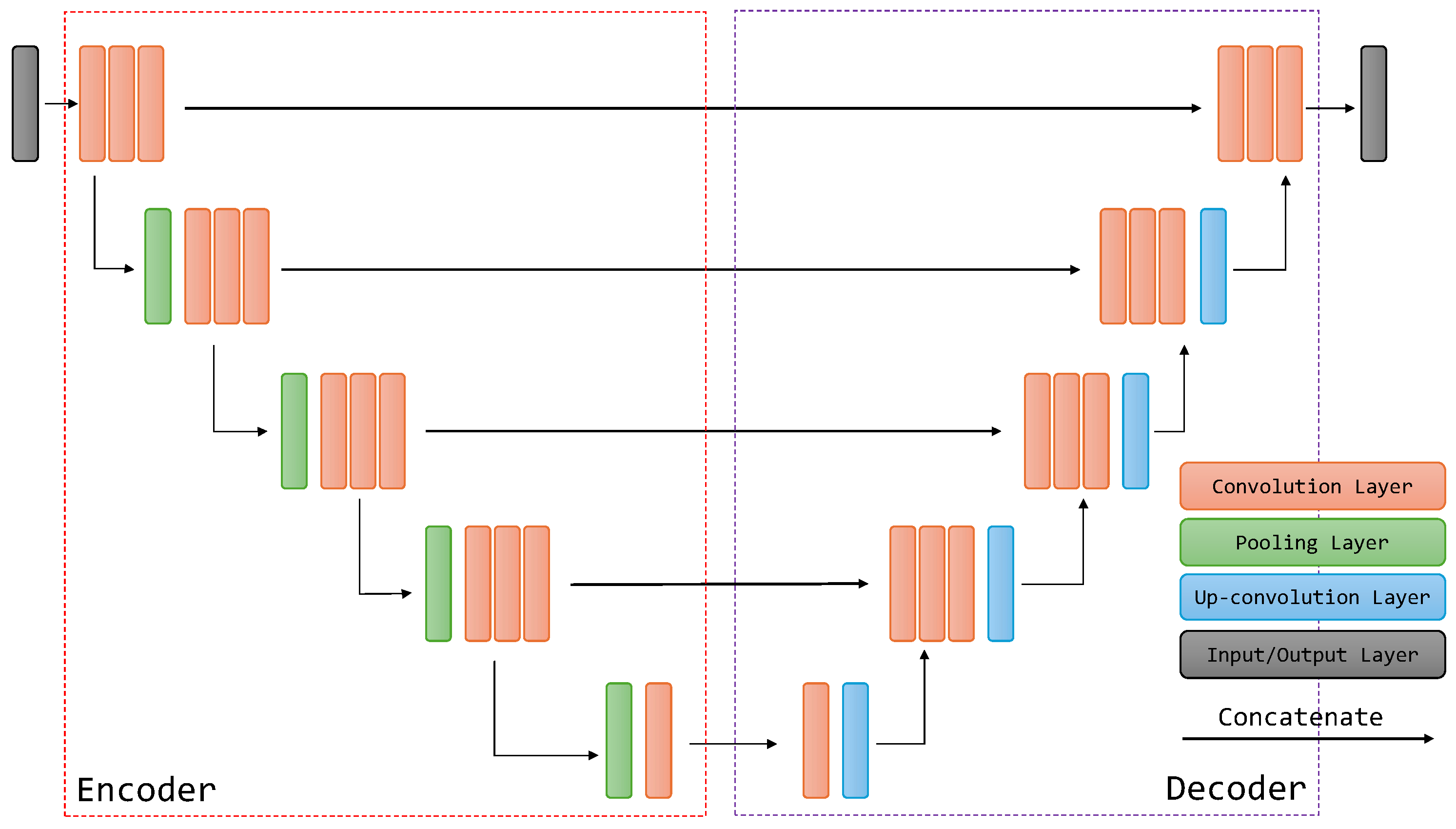
U-Net is a convolutional neural network architecture designed for semantic segmentation tasks, particularly in medical image analysis [23]. U-Net is characterized by a U-shaped architecture that consists of a contracting path for feature extraction (encoder) followed by an expansive path for precise localization (decoder) as depicted in Figure 1.
The encoder processes the input image and extracts features by using repeated stacks of convolutional layers with pooling operations (like max pooling). Pooling operations reduce the spatial resolution of the image while capturing higher-level features. Each stack typically increases the number of filters, allowing for learning more complex features. The decoder aims to recover the spatial resolution while preserving the extracted features by using upsampling operations (like transposed convolution) to increase the resolution. Each upsampling step combines the upsampled feature map with a corresponding feature map from the contracting path (via skip connections). Skip connections directly provide detailed information from the earlier stages, helping the decoder accurately localize features. The decoder culminates in a final convolutional layer with several filters equivalent to the predefined number of segmentation classes. This layer effectively acts as a classifier, generating a probability map as its output. Each pixel value within this map represents the probability of that specific pixel belonging to a particular class.
The combination of contracting and expanding paths with skip connections allows U-Net to learn both high-level semantic features and low-level spatial details crucial for accurate segmentation. U-Net architecture is known to perform well even with limited training data compared to other segmentation models [23]. This is partly due to the effective use of skip connections. U-Net can be adapted to various segmentation tasks by changing the number of classes and the final layer configuration. Overall, U-Net’s U-shaped structure with its contracting and expanding paths makes it a powerful and widely used architecture for semantic segmentation tasks.
The U-Net architecture is flexible and allows for the incorporation of different encoders as feature extractors/backbones. One of the strengths of U-Net is its adaptability to various encoder structures. The original U-Net architecture is often modified by replacing the default encoder with pretrained models like VGG and ResNet, depending on the specific requirements of the tasks or datasets at hand. In this study, three distinct backbone networks are utilized: Multi-Axis Vision Transformer (MaxViT) [44], ConvFormer [45], and EfficientNet [46].

2.2.1. Multi-Axis Vision Transformer

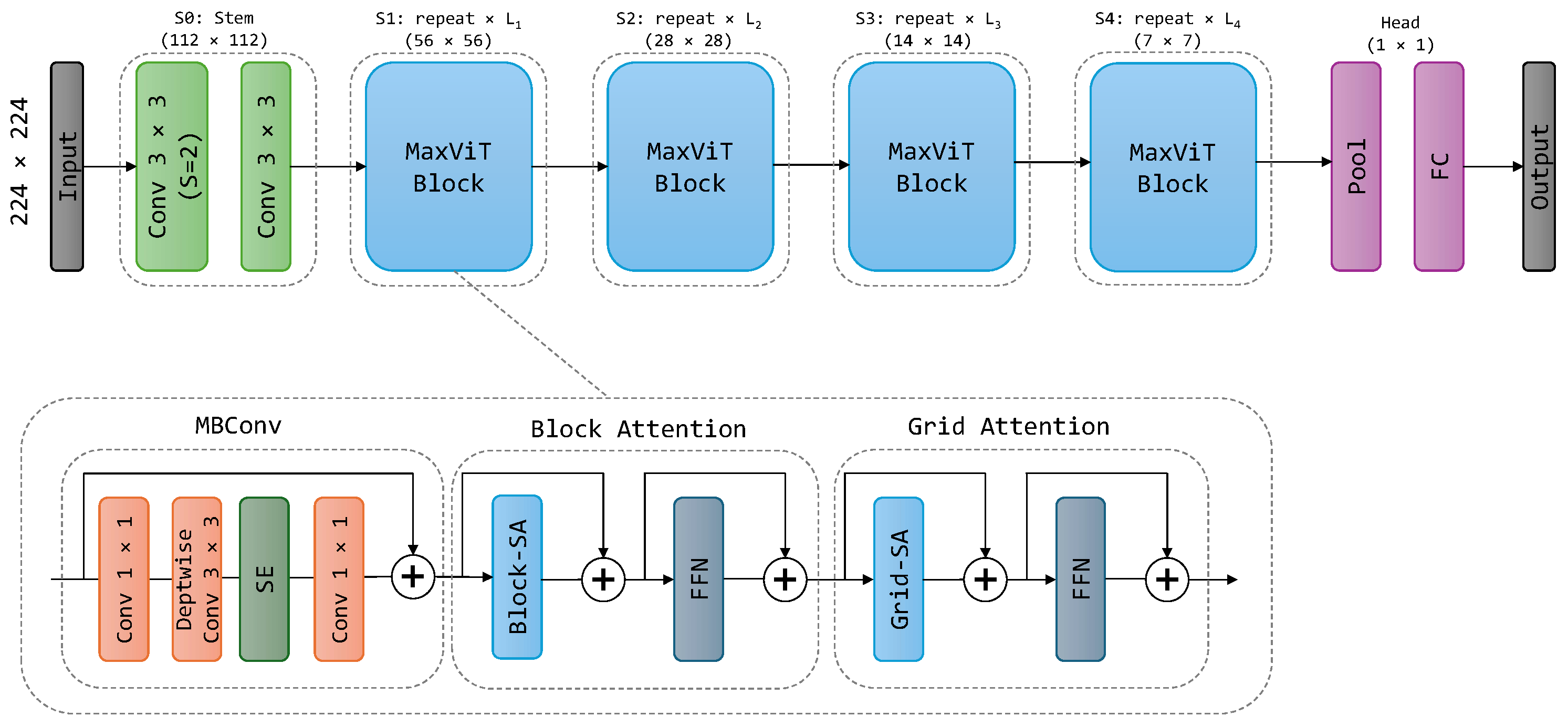
MaxViT is a recent advancement in vision transformer architectures that addresses the challenge of capturing both local and global information within an image [44]. MaxViT utilizes a hierarchical architecture where each stage in the hierarchy consists of a MaxViT block, which combines a multi-axis self-attention (Max-SA) block with a convolutional layer. This combination leverages the strengths of both approaches: Max-SA for global context and convolutions for efficient local feature extraction. The use of Max-SA makes MaxViT computationally efficient compared to full self-attention in standard ViTs [47].
The architecture of the MaxViT network is illustrated in Figure 2. The network begins by downsampling the input through Conv3x3 layers in the stem stage (S0). The body of the network contains four stages (S1–S4), with each stage having half the resolution of the previous one with a doubled number of channels (hidden dimensions). The MaxViT model can be scaled up by increasing the number of blocks per stage and the channel dimension. There are several MaxViT variants including MaxViT-T, MaxViT-S, MaxViT-B, MaxViT-L, and MaxViT-XL. These variants progressively increase in complexity (number of blocks and channels) and likely performance, potentially reaching a trade-off between accuracy and efficiency [44]. In this study, we use MaxViT-S as an encoder in the U-Net architecture. MaxViT’s architecture allows for easy scaling to handle large datasets and complex tasks. By combining efficient global attention with the ability to capture local details, MaxViT offers a promising approach for various computer vision applications, including the task of semantic segmentation explored in this work.

2.2.2. ConvFormer

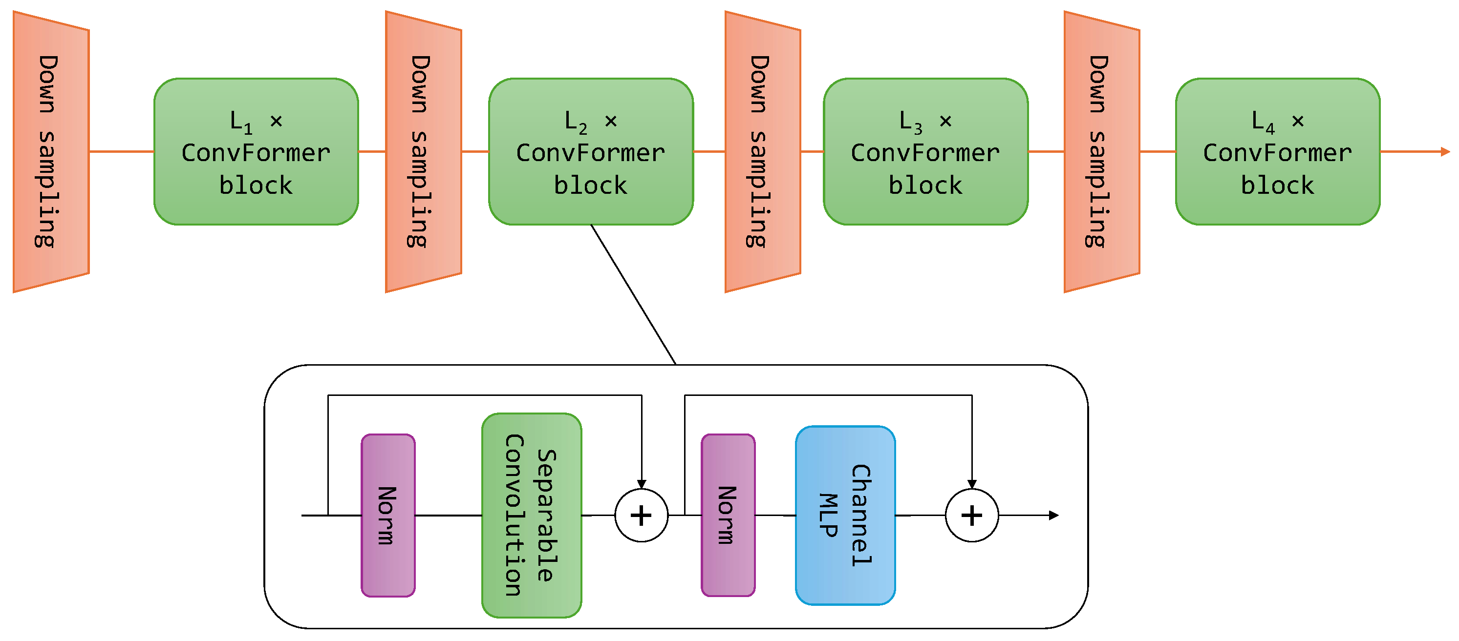
The MetaFormer concept is not tied to a particular model; rather, it is a generalized architecture abstracted from the transformer, omitting the specification of token mixers [48]. The instantiation of MetaFormer into specific models occurs by specifying concrete token mixers as modules. One way to instantiate the token mixer within the MetaFormer is by using separable depthwise convolutions. This specific implementation results in a model called ConvFormer [45]. ConvFormer leverages the MetaFormer structure for efficient feature processing but relies solely on convolutional operations, making it functionally a type of CNN. ConvFormer adopts a hierarchical architecture of 4 stages [49], as illustrated in Figure 3. Based on the number of channels and the number of blocks, several model configurations of different sizes are defined: ConvFormer-S12, ConvFormer-S24, ConvFormer-S36, ConvFormer-M36, and ConvFormer-M48. In this study, we adopt the ConvFormer-M36 as an encoder in the U-Net architecture. The notation “M36” means the model is of medium size of embedding dimensions (the total number of channels in all four stages) with 36 ConvFormer blocks in total. ConvFormer demonstrates superior performance compared to the robust CNN model ConvNeXt [50] and achieves comparable accuracy to another powerful CNN model, EfficientNetV2-L [51]. Additionally, ConvFormer surpasses several strong attention-based or hybrid models. Notably, ConvFormer-M36 outperforms Swin-B [52] and CoAtNet-2 [53] while utilizing fewer parameters.

2.2.3. EfficientNet

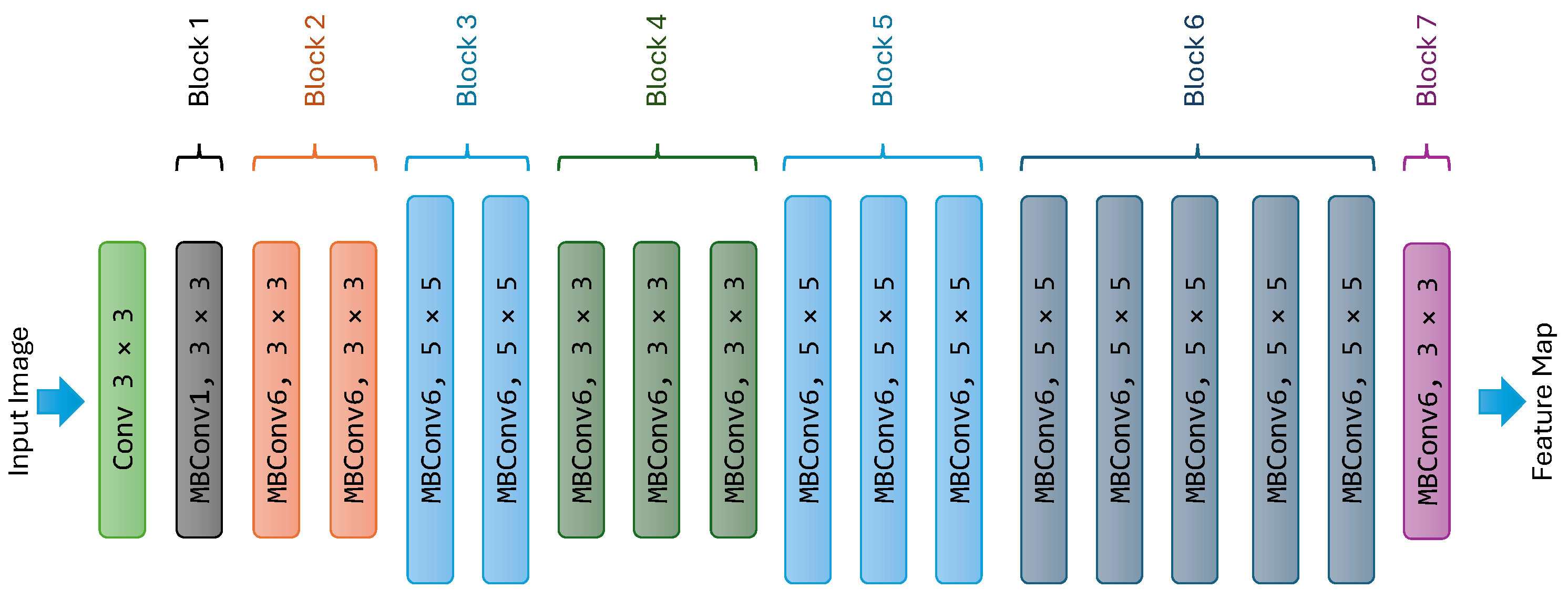
EfficientNet is a family of convolutional neural network (CNN) architectures designed to achieve state-of-the-art accuracy while maintaining computational efficiency [46]. It addresses the challenge of finding an optimal balance between three key factors influencing model capacity and performance: depth, width, and resolution. EfficientNet proposes a novel scaling method that systematically balances these three factors. It utilizes a compound coefficient that uniformly scales depth, width, and resolution in a principled way. This approach ensures efficient resource allocation and avoids overemphasizing any single factor. EfficientNet models have achieved remarkable accuracy on various image classification tasks, often surpassing previous CNN architectures [5]. Several EfficientNet models can be scaled from the baseline EfficientNet-B0 model using different compound coefficients [46], offering a good trade-off between accuracy and resource consumption. Variants like B1 to B7 progressively increase in complexity. The EfficientNet architecture relies on the MBConv layer, which is an inverted residual block. Figure 4 illustrates the basic building blocks of EfficientNet-B0, highlighting the MBConv layers.
The specific choice of the EfficientNet variant depends on the task at hand and the available computational resources. By offering a spectrum of complexity levels, EfficientNet provides a versatile set of CNN architectures for various image recognition applications [5,46]. In this study, we adopt EfficientNet-B7 as an encoder in the U-Net architecture.

2.2.4. Ensemble Method

Ensemble learning is a powerful technique in machine learning that involves combining the predictions of multiple models to achieve better performance than any single model could on its own [54]. Ensemble methods can help reduce the variance of the predictions, making the model less prone to overfitting or poor performance on unseen data. Ensembles are also less susceptible to errors or biases present in any single base model. Ensemble learning offers a valuable approach to enhancing the performance and robustness of deep learning models. Strategically combining multiple models has the potential to yield superior results across a range of deep learning tasks, such as image classification [55], semantic segmentation [56,57], and object detection [58,59]. The ensemble approach in the context of deep learning starts by training multiple deep learning models, often referred to as base models. These base models can have identical architectures trained with different initial weights or hyperparameters to promote diversity in the learning process, or they may have different architectures altogether to leverage the strengths of diverse approaches to feature extraction and representation. Once trained, the predictions from each base model are combined in some way to generate the final ensemble predictions. Common combination strategies are averaging, weighted averaging, and voting [60].
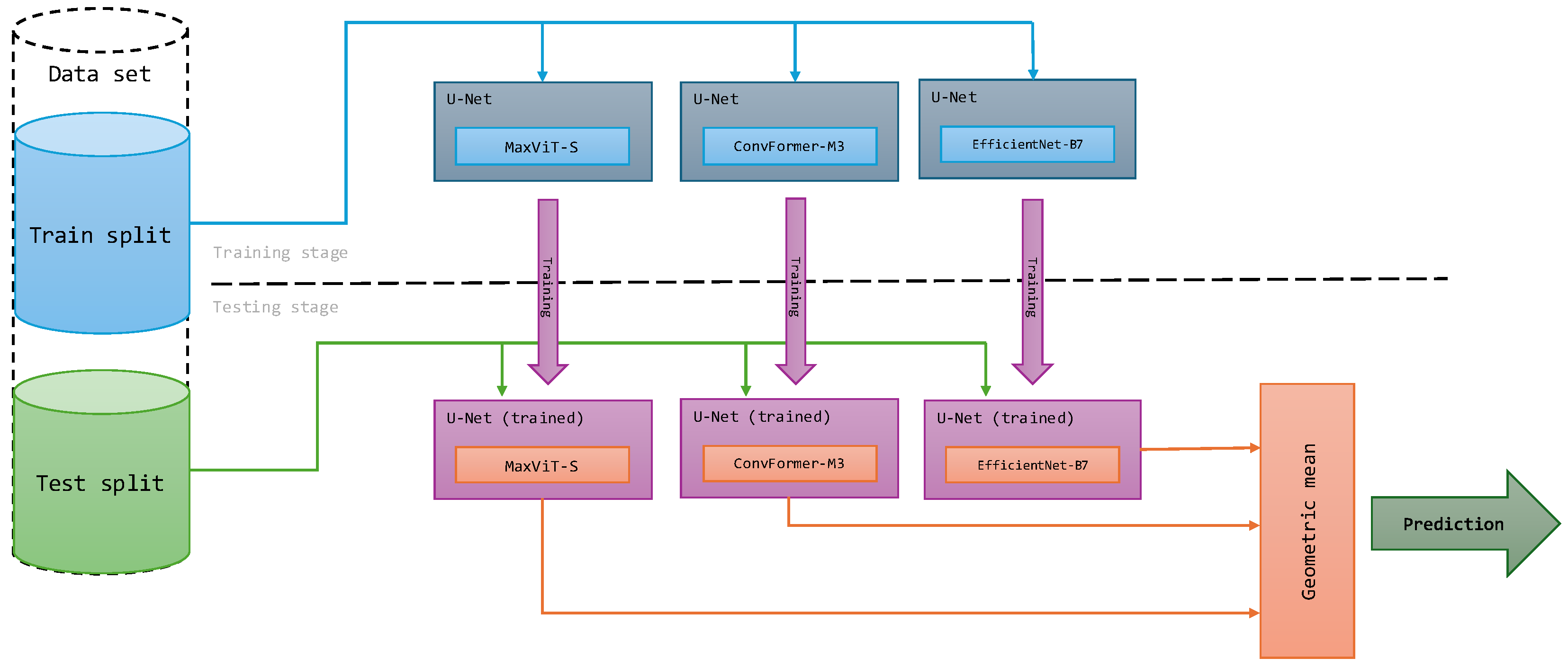
This paper investigates the potential of ensemble learning for semantic segmentation tasks in remote sensing imagery. We built the ensemble by combining base models as diversely as possible. The key strength lies in the diversity of the employed backbones in the base models. The ensemble utilizes U-Net architecture with three distinct backbone networks: Multi-Axis Vision Transformer (MaxViT), ConvFormer, and EfficientNet. The full setup is illustrated in Figure 5. Each backbone network possesses unique advantages. For example, MaxViT is a hybrid vision transformer architecture, ConvFormer utilizes convolutional layers within a transformer framework, and EfficientNet is a CNN architecture known for its balance between accuracy and efficiency. This diversity in the feature extraction process allows the ensemble to capture a richer and more comprehensive understanding of the image, potentially leading to improved segmentation performance and more robust and accurate segmentation results.
To generate the final segmentation maps, we employ a geometric mean ensemble strategy, assuming the ensemble has k (in our experiments, k = 3 ) base models, denoted by [ M 1 ( x ) , , M k ( x ) ] , where x is the input image. Each model outputs a raw score vector, denoted as [ z 1 , , z k ] . We apply the s o f t m a x function to each raw score vector z i to convert them into probability distributions (typically between 0 and 1) over the class labels as expressed in Formula (1).
p i ( x ) = s o f t m a x ( z i ) = e z i j = 1 k e z j
where p i ( x ) represents the probability vector for the i-th base model given the input image x. The final probability scores, E ( x ) , are obtained by combining the probability scores for each base model using the geometric mean function as in Formula (2). The segmentation map is calculated by applying the a r g m a x function on the ensemble probability scores E ( x ) .
E ( x ) = i = 1 k p i ( x ) 1 k
In essence, this work explores the potential of ensemble learning to enhance the capabilities of U-Net architecture for semantic segmentation tasks in remote sensing imagery. By utilizing a diverse set of backbones and a geometric mean ensemble strategy, we aim to achieve superior segmentation performance compared to existing/published methods.

2.3. Experimental Setup

This study investigates the performance of three U-Net variations for semantic segmentation of remote sensing images. Each variant utilizes different pretrained encoders: MaxViT-S, ConvFormer-M36, and EfficientNet-B7. The encoders are pretrained on the ImageNet-1K dataset, which helps to learn general visual features that can be beneficial for semantic segmentation tasks. Additionally, we assess the effectiveness of an ensemble approach, where the predictions from base models are combined for improved performance. In this ensemble, the final prediction for each pixel is derived by calculating the geometric mean of the probabilities predicted by each U-Net variant.
The models were trained using the training set, with parameter selection/search performed using the validation set. To overcome overfitting, we performed early stopping on the validation set if no improvements in the validation loss were observed over 20 epochs. The best checkpoint/model found (with the highest evaluation metric) was saved and then applied to the original test set to obtain the final assessment of the predictive performance. The maximum number of epochs was set to 100.
In our experiments, we used a fixed value for the batch size, set to 12. For optimization, we employed the AdamW optimizer and a learning rate set to 0.0001 [61]. Next, we used a learning rate scheduler that used a polynomial decay schedule. It is commonly observed that a monotonically decreasing learning rate, whose degree of change is carefully chosen, results in a better performing model. This schedule applied a polynomial decay function to an optimizer step, given a provided initial_learning_rate (1 × 10⁻⁴), to reach an end_learning_rate (1 × 10⁻⁷) in the given decay_steps. We used a combination of cross-entropy loss and dice loss to achieve a more balanced approach to semantic segmentation. Cross-entropy loss measures the pixel-wise similarity between the predicted and ground-truth masks, while the dice loss ensures accurate boundary localization. The combination of these loss functions is effective in achieving both accurate object localization and overall segmentation accuracy.
To further enhance the model’s robustness, we incorporated data augmentation techniques during training. The process involved random horizontal and vertical flips, followed by random rotation and random changes in the brightness and contrast. Additionally, we randomly selected one of the following transformations to apply: contrast limited adaptive histogram equalization to the input image, grid distortion, or optical distortion [62]. Finally, normalization was applied using the mean and standard deviation derived from the ImageNet-1k dataset. The augmentation strategy for the UAVid dataset differed, as it excluded vertical flipping and random rotation techniques. For the LoveDA dataset, we first utilized the RandomCrop transformation to randomly extract smaller image patches from the original images [62]. Specifically, we cropped 512 × 512 pixel regions from the original LoveDA images, which have a larger dimension of 1024 × 1024 pixels. We ensured that all datasets had a consistent input resolution of 512 × 512 pixels for training the models. However, during the evaluation of validation or test data, the input images were only normalized.
The inference approach used depends on the image size of the test set within each dataset. The inference for the LoveDA, LandCover.ai, and ISPRS Potsdam datasets was directly applied to the entire image due to their relatively small resolution. For the INRIA and UAVid datasets, because of the larger test images, we employed a sliding-window inference technique [63]. This method partitions the image into smaller overlapping patches, processes each patch with the model, and then assembles the predictions to create the final segmentation map. The sliding window was configured with dimensions of 1024 pixels, and the overlap was set to 128 pixels. For areas covered by multiple sliding windows, the final prediction was determined by averaging the predictions from each window. This distinction ensured efficient processing for smaller images while effectively handling larger ones with overlapping patches to capture the entire scene. Moreover, we implemented test-time augmentation (TTA) through horizontal flipping and rotation. The final prediction was computed as the mean of predictions obtained from both the original and augmented images.
In terms of evaluation measures for predictive performance, we report the label-wise intersection over union ( I o U ) as an evaluation measure, which denotes the area of the overlap between the ground truth and predicted label divided by the total area. We also report the mean intersection over union ( m I o U ) averaged across the different labels. All models were trained on NVIDIA A100-PCIe GPUs with 40 GB of memory running CUDA version 11.5. We configured and ran the experiments using the deep learning framework PyTorch Lightning [64].

3. Results and Discussion

The summarized results of the base U-Net models and the ensemble models across the different evaluation datasets are shown in Table 2. We report the mean intersection over union (%) and also report the rank of the models, averaged over the respective datasets. For the INRIA dataset, the provided metric is the intersection over union (%) specifically for the building label, which is a common practice in building extraction [40]. Notably, the U-Net ensemble models ranked the best overall and achieved the best performance on six (out of the six) tasks/datasets. Among the base models, those utilizing MaxViT-S as a backbone ranked second, closely followed by the U-Net models with EfficientNet-B7 as a backbone. While the U-Net models featuring the ConvFormer-M36 backbone ranked last, they demonstrated comparable performance across all datasets.
The ensemble models consistently outperform across all datasets. For the LoveDA dataset, the achieved mIoU stands at 57.36%, marking the best result and securing the top rank on the publicly available leaderboard of the LoveDA semantic segmentation challenge. Similarly, for the UAVid dataset, the mIoU reaches 73.34%, which also represents the best reported result to date for this dataset. For the LandCover.ai datasets, the ensemble surpasses all previously reported results, achieving mIoU values of 88.02%. We analyzed the segmentation performance on the Potsdam dataset in two cases, with and without clutter (background). The label clutter is the most challenging as it can contain anything except for the five main labels defined for this dataset. Our U-Net ensemble stands out as a robust segmentation model, achieving top performance in both scenarios, with and without clutter, boasting mIoU values of 80.82% and 89.9%, respectively. Moreover, the obtained IoU value of 81.43% for the INRIA dataset aligns with the best-performing methods and reported results observed on the contest platform hosted by the dataset creators. These results strongly validate the effectiveness of our proposed ensemble approach in enhancing semantic segmentation performance on remote sensing imagery. Table 3 presents the performance of various backbone combinations on the selected semantic segmentation datasets. While all combinations outperform the base models, the ensemble utilizing all three backbones (MaxViT, ConvFormer, EfficientNet) consistently achieves the best results.
Having established the overall effectiveness of U-Net models, both base models and ensemble models, we now examine how well they perform on each dataset. This analysis aims to identify the potential strengths and weaknesses of the models across different types of remote sensing imagery and segmentation tasks. Subsequently, we explore any notable observations or patterns based on the performance of each specific dataset. Our analysis includes per-label IoU values, confusion matrices, and sample inference masks for each dataset. These insights will aid in understanding performance fluctuations across different labels or regions within the images (e.g., urban versus rural areas) and pinpoint potential challenges such as data imbalances or complex object shapes. We also present a detailed comparison of our models performance against established methods/models for all considered remote sensing image datasets.
In Table 4, we report performance comparisons with existing methods on the test set of the LoveDA dataset. This comparison is based on the IoU metric calculated for each semantic class/label. Our models (base and ensemble) consistently outperform existing state-of-the-art methods. Notably, this includes competitive approaches like AerialFormer-B [38], DC-Swin [65], multitask pretraining using the InternImage-XL model [66], UperNet (Swin small) [27], and the foundation model trained with UperNet and a vision transformer as a backbone [67]. To explore the impact of encoder selection on performance, we compared our trained U-Net models to a variant equipped with a ResNet50 encoder. The U-Net model with a ResNet50 encoder achieves an mIoU value of 47.84%. Our U-Net models demonstrate significant improvements: the MaxViT backbone outperforms this result by 8.32% in mIoU, the ConvFormer by 6.96%, and EfficientNet by 7.23%. This demonstrates the effectiveness of our backbone selection.
The top-performing model is the U-Net ensemble, achieving an mIoU value of 57.36%, marking a substantial improvement of 2.81% over existing state-of-the-art methods. This result also secures the highest rank on the publicly available leaderboard of the LoveDA semantic segmentation challenge. Notably, the U-Net ensemble outperforms the existing methods by 2.33% IoU for the road label, 2.26% IoU for the barren label, 1.39% IoU for the forest label, 1.82% IoU for the agriculture label, 0.11% IoU for the water label, and 1.29% IoU for the background label. The U-Net ensemble model exhibits a lower IoU value only for the building label, with a decrease of 1.48% compared to existing methods.
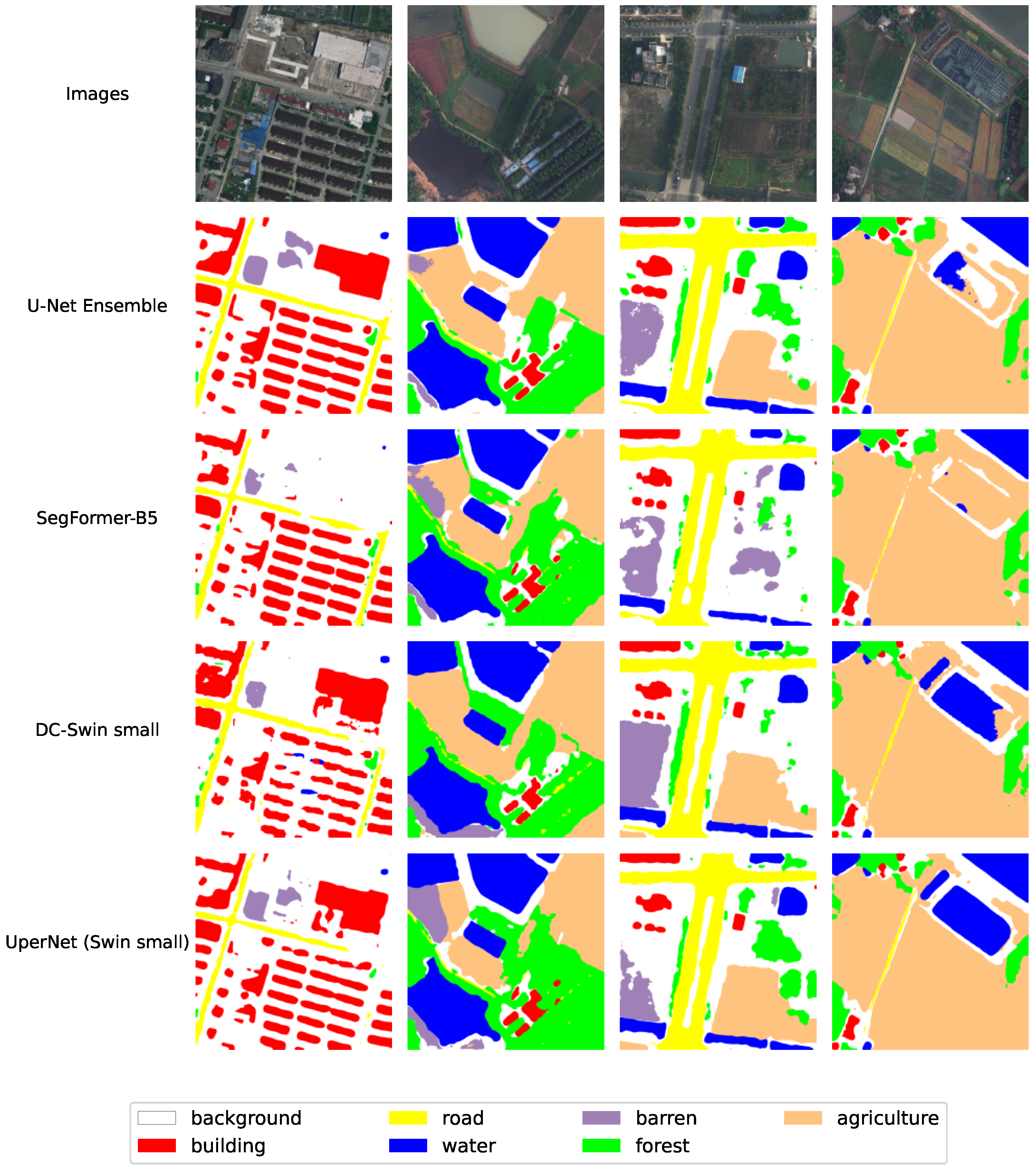
A confusion matrix was not calculated for this dataset as the ground-truth masks for the test images are not publicly accessible. Figure 6 displays sample images alongside the inference masks generated by the U-Net ensemble, the best-performing model, and other models for comparison. The mIoU value of 57.36% for this dataset indicates its high level of difficulty. The regions labeled as background exhibit significant intraclass variance due to the complexity of the scenes, leading to substantial false alarms. Identifying small-scale objects like buildings and scattered trees poses challenges. Additionally, distinguishing between forest and agricultural labels is difficult due to their similar spectra. However, the water label achieves the highest IoU value, suggesting good recognition performance for this label.
Table 5 presents a performance comparison of the UAVid dataset test set, evaluated using the intersection over union (IoU) metric for each semantic class/label. Our ensemble model surpasses existing state-of-the-art methods such as EMNet [68], DCDNet [69], and UperNet (Swin small) [27], while our base U-Net models achieve competitive results. We investigated the influence of encoder selection on performance by comparing our U-Net models to a variant equipped with a ResNet50 encoder. This baseline U-Net achieved an mIoU value of 67.22%. However, even stronger results were obtained by employing more powerful backbones within the U-Net architecture. The MaxViT backbone significantly outperformed the ResNet50 by 4.66% in mIoU, while ConvFormer and EfficientNet also achieved improvements of 3.57% and 4.2%, respectively. These findings demonstrate the effectiveness of our backbone selection strategy in boosting U-Net’s performance for remote sensing semantic segmentation tasks. Our top-performing U-Net ensemble achieves a state-of-the-art mIoU of 73.34%, exceeding the methods presented in Table 5 and the best results of 73.21% mIoU from the public UAVid competition, https://competitions.codalab.org/competitions/25224 (accessed on 5 June 2024).
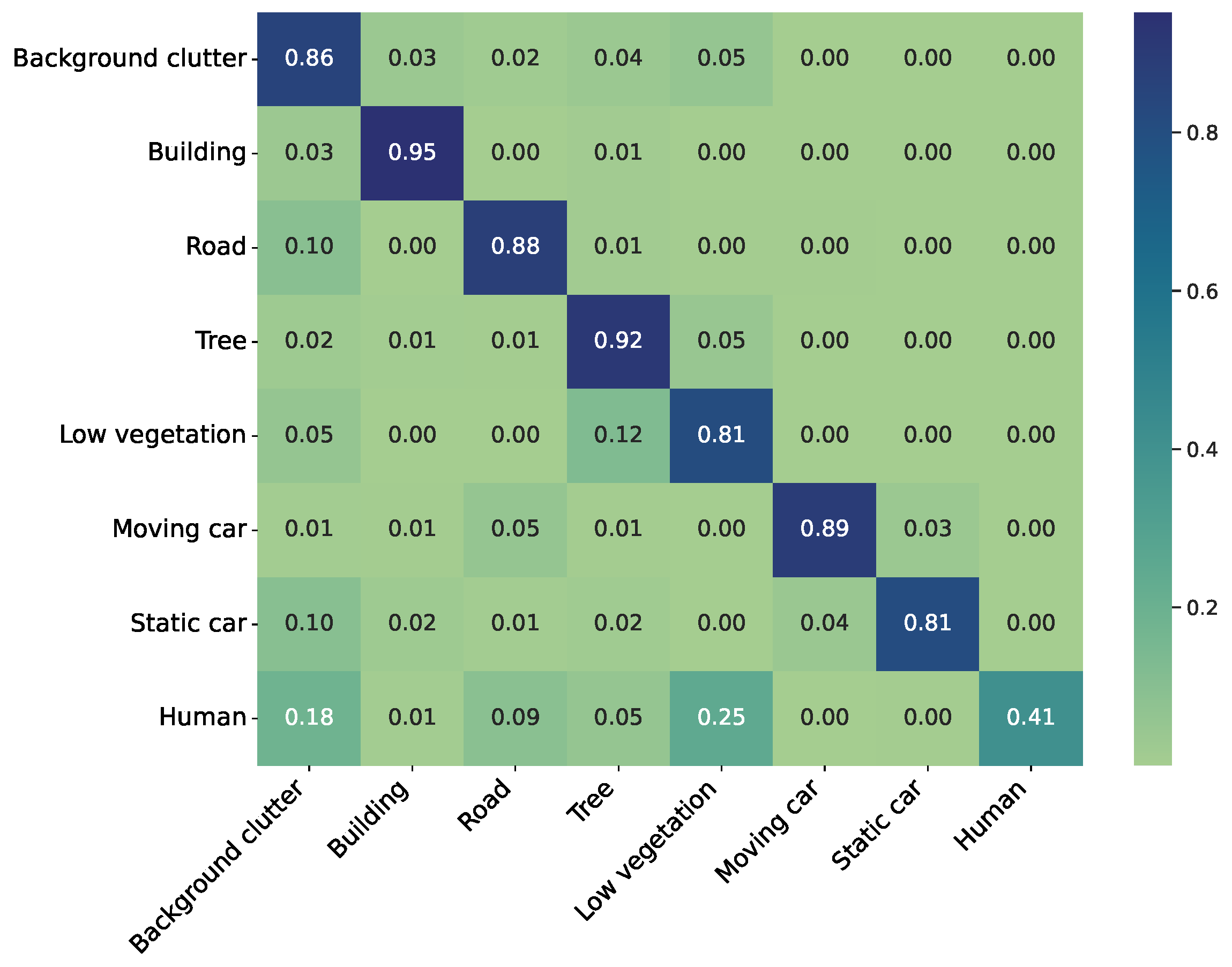
Examining the IoU values, it becomes evident that the most accurate predictions are achieved for the building label. Moreover, satisfactory results are obtained for the road, tree, and moving car labels. The label human exhibits the lowest performance. The confusion matrix calculated for the U-Net ensemble as the best-performing model is visualized in Figure 7. The confusion matrix reveals the frequent misclassifications by the model. Notably, it tends to confuse the labels moving car and static car, as well as tree and low vegetation. This is rather expected given the semantic similarity between these labels. Additionally, there is a tendency to misclassify the human label as the low vegetation label, likely a result of pixel overlap between these two labels. There are misclassifications with the background clutter label for nearly all labels, as expected. This is because diverse objects and regions not belonging to any specific label are designated with the background clutter label.
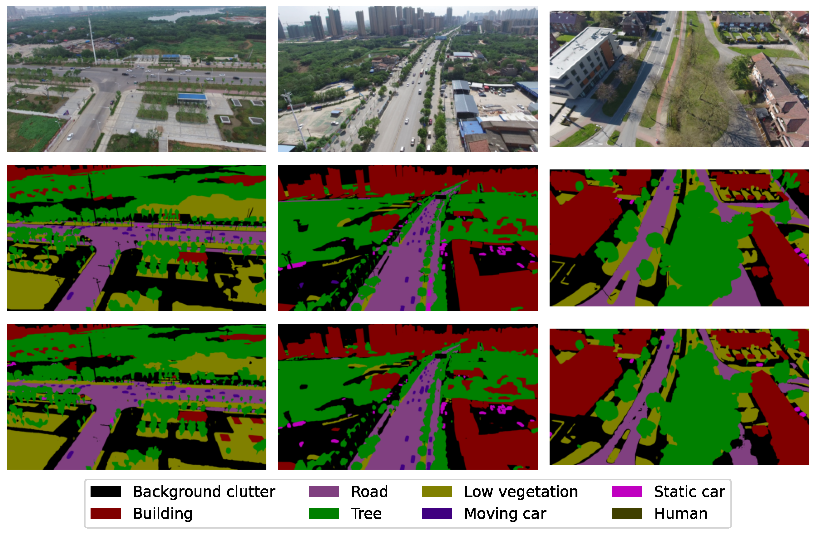
Figure 8 shows example images and ground-truth masks from the UAVid dataset. Additionally, it presents the inference masks generated by the U-Net ensemble model. Despite the high scene complexity, characterized by the number of objects and varied object configurations in the UAVid dataset, the U-Net ensemble model demonstrates excellent performance. Figure 9 showcases a cropped region of an example image along with its corresponding ground-truth mask, featuring the labels human and moving cars. The predicted mask, shown as the last image in Figure 9, is generated by the U-Net ensemble model. A comparison between the ground-truth mask and the predicted mask reveals segments where the model misclassifies moving cars as static cars. In this particular scenario, distinguishing between these two labels is challenging because, for instance, the cars are stationary, waiting at the pedestrian crossing. Additionally, there is a lack of fine-grained segmentation for the human label due to overlapping and dense objects/segments marked with this label in the ground-truth mask.
In Table 6, we report performance comparisons with existing methods on the test set of the LandCover.ai dataset. This comparison is based on the IoU metric calculated for each semantic class/label. Our models (base and ensemble) consistently outperform existing state-of-the-art methods. Notably, this includes competitive approaches like DC-Swin small [65], UperNet (Swin small), and SegFormer-B5 [33]. In the comparison for this dataset, we also included a U-Net model with ResNet50 as the backbone, achieving an mIoU value of 85.66%. Compared to this result, our U-Net models show notable improvements with different backbones: a 1.75% mIoU gain for MaxViT, a 1.98% gain for ConvFormer, and a 1.4% gain for EfficientNet. These results underscore the advantages of our chosen backbones. Our top-performing model is the U-Net ensemble, achieving an mIoU value of 88.02%, marking an improvement of 0.64% over existing state-of-the-art methods.
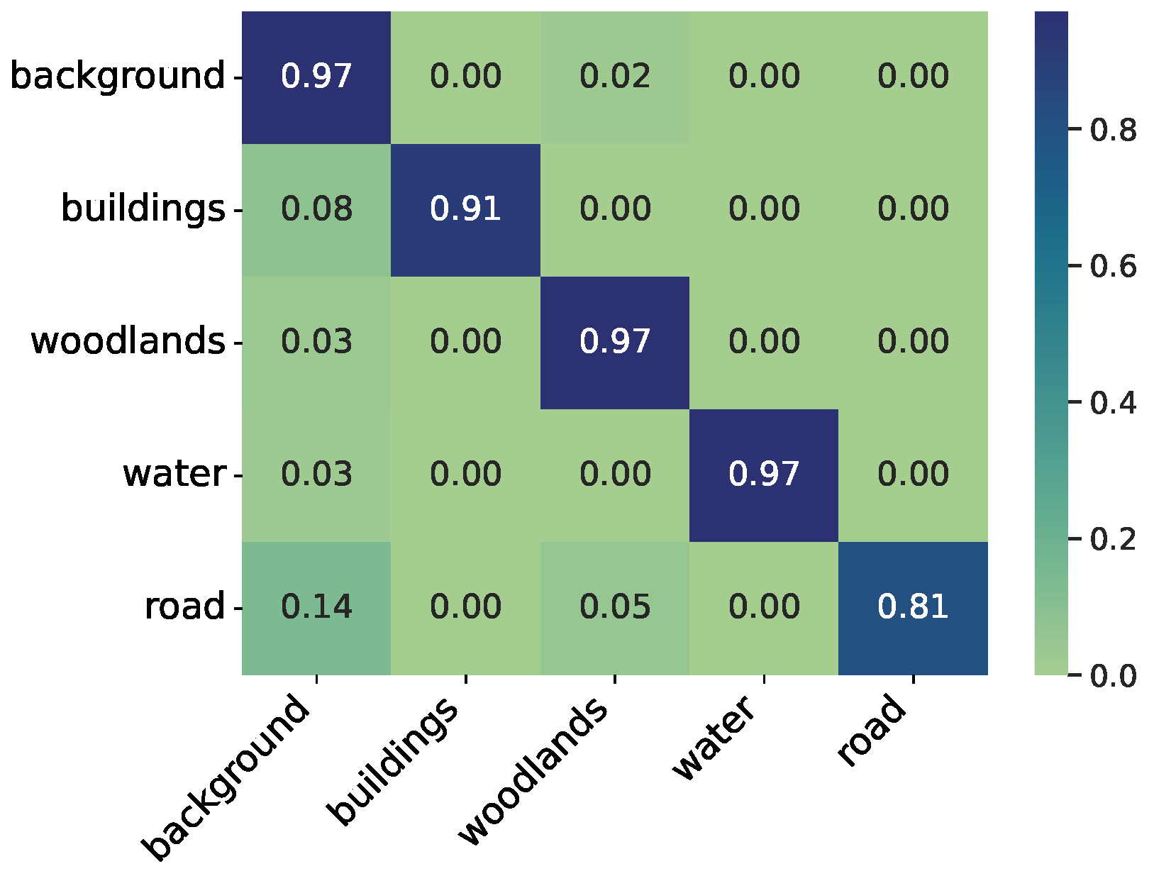
The IoU values for the labels road and building are lower compared to the other labels. These labels are more challenging in the context of semantic segmentation because they are usually narrow, in the case of roads, or often small, in the case of buildings. Additionally, they are sometimes obscured by other objects, such as trees. Figure 10 illustrates the confusion matrix for the LandCover.ai dataset calculated for the U-Net ensemble model. The confusion matrix further supports this observation, indicating that the road label is frequently misclassified as woodlands, and in general, all labels exhibit confusion with the background label, as expected due to its diverse composition, which may include fields, grass, or pavement.
Figure 11 shows example images and ground-truth masks from the LandCover.ai dataset. Additionally, it displays the inference masks generated by the U-Net ensemble, the best-performing model, and other models for comparison. The identified regions within the inference masks typically exhibit smoother boundaries, aligning well with reality, particularly in the context of woodlands and water. However, this smoothness can lead to inaccuracies for buildings, potentially omitting smaller structures and producing slightly less defined/precise building edges/boundaries. Conversely, the model excels at identifying individual trees that might have been missed by human annotators.
We evaluate the segmentation performance on the Potsdam dataset under two conditions: with and without clutter. For this dataset, we report per-label F1 scores, mean F1 scores, and mean intersection over union (IoU). We include F1 scores in this comparison because previous studies on this dataset utilized this metric to assess predictive performance. The results for the two evaluation scenarios are presented in Table 7 and Table 8. In this experimental setup, the analysis indicates that U-Net (ConvFormer-M36) and the U-Net ensemble achieved the highest scores in mIoU and mF1 metrics when the clutter label was excluded from consideration. However, when the clutter label was included, U-Net (EfficientNet-B7) and the U-Net ensemble emerge as the top performers. Interestingly, the exclusion of clutter seems to reduce ambiguity among the remaining labels.
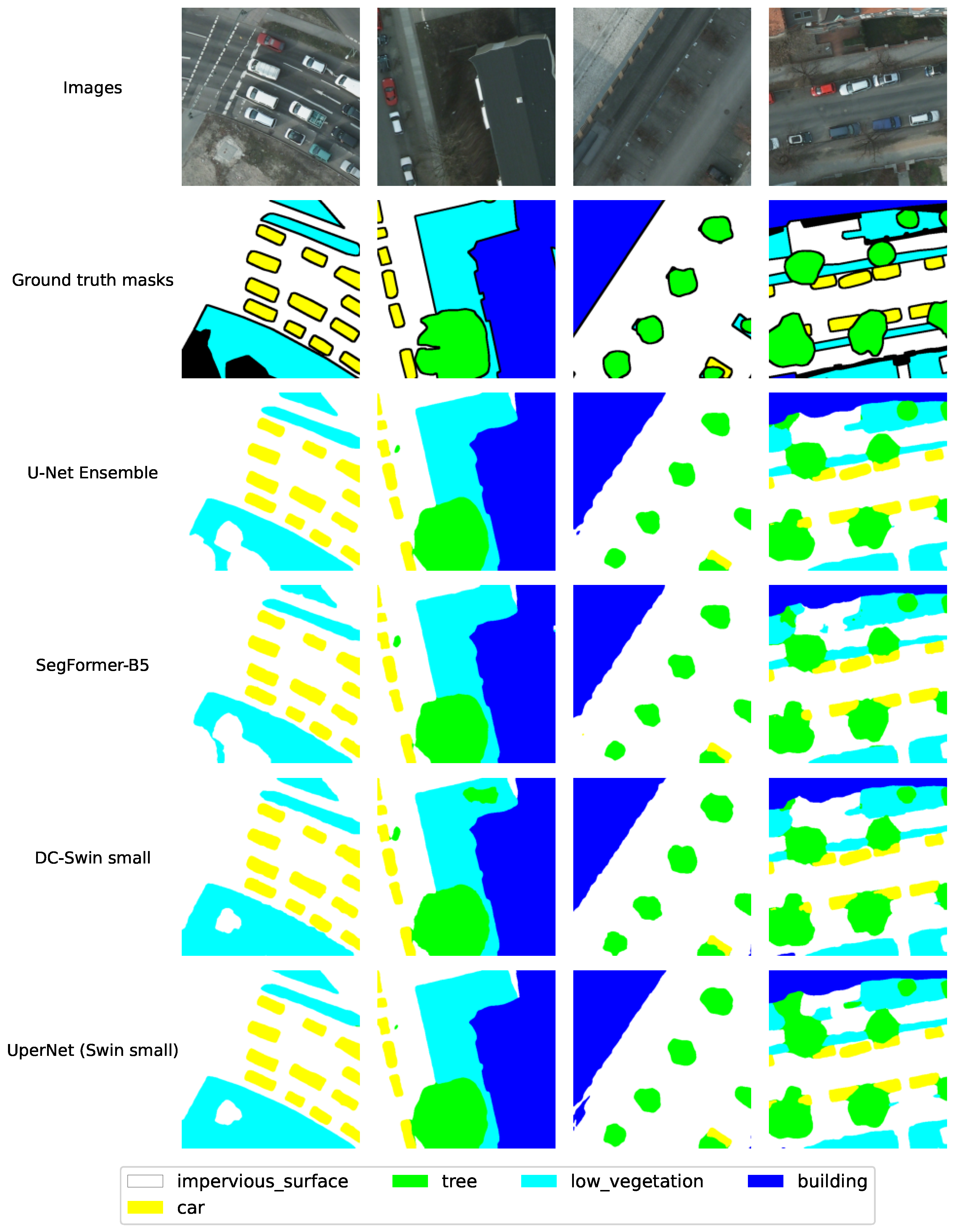
Figure 12 shows example images and ground-truth masks from the Potsdam dataset. Additionally, it displays the inference masks generated by the U-Net ensemble, the best-performing model, and other models for comparison. The U-Net ensemble model exhibits remarkable resilience, achieving excellent performance despite the high scene complexity of the Potsdam dataset. The confusion matrices for the Potsdam dataset (with and without clutter) are visualized in Figure 13. The clutter label in the Potsdam dataset presents a unique challenge as it encompasses anything outside the five main categories. This ambiguity can lead to confusion with labels like impervious_surface, low_vegetation, and building. Excluding the clutter label significantly reduces ambiguity among the remaining labels. This is evident in the F1 values exceeding 90% for all the labels when clutter is ignored. As expected, some confusion persists between tree and low_vegetation labels, likely due to their inherent similarities.
For the INRIA dataset, the provided metric is the intersection over union (%) specifically for the building label, which is a common practice in building extraction [40]. Our model achieves a competitive IoU value of 81.43% on the building extraction task, even without incorporating postprocessing techniques for boundary refinement. While this aligns with current state-of-the-art results (the highest reported on the contest platform being 81.91%), there is room for further improvement. For instance, the UANet method [40] achieves an IoU of 83.08% by introducing uncertainty awareness into the network. This allows UANet to maintain high confidence in predictions across diverse scales, complex backgrounds, and various building appearances. As future work, we plan to explore similar uncertainty-handling techniques to potentially boost the performance of our models. Figure 14 showcases close-ups of the segmentation outcomes on the test set. The U-Net ensemble model adeptly identifies buildings across diverse images, showcasing its capability to detect structures of varying sizes and shapes.
Balancing Performance and Efficiency

Our approach leverages medium-sized backbones, MaxViT-S (∼69M parameters), ConvFormer-M36 (∼57M parameters), and EfficientNet-B7 (∼66M parameters), within the U-Net architecture. This choice strikes a balance between performance and computational efficiency. Notably, the individual base models achieve competitive results on most datasets, showcasing the effectiveness of these backbones. For instance, compared to state-of-the-art methods like AerialFormer-B (∼114M parameters), SegFormer-B5 (∼84M parameters), DC-Swin small (∼67M parameters), multitask pretraining using the InternImage-XL model (∼335M), and UperNet with Swin (small variant) (∼81M parameters), our models achieve similar performance with a comparable number of parameters. This demonstrates that our chosen medium-sized backbones offer a strong trade-off between accuracy and resource consumption.
To push the performance of the base U-Net models even further, we introduce a three-model ensemble strategy. This approach capitalizes on the complementary strengths of each backbone by combining their diverse feature representations, aiming to surpass the capabilities of base models. Ensemble methods present a trade-off: they can boost performance but come with a higher computational burden. Limiting the ensemble to three models ensures a good balance between performance gains and computational cost. This selection provides a diverse set of feature extraction capabilities while maintaining computational tractability. To further improve efficiency, we can explore techniques for optimizing the inference time of the base models. These techniques include pruning the model architecture [72] and quantizing the network parameters [73].

4. Conclusions

In this paper, we explored the effectiveness of incorporating strong backbones within the U-Net architecture to enhance the semantic segmentation of remote sensing imagery. We investigated three distinct backbone networks—Multi-Axis Vision Transformer, ConvFormer, and EfficientNet. These backbones extract complementary features, leading to a richer understanding of the scene. Further, we introduced an ensemble learning approach that leverages the unique representations learned by each backbone, resulting in more robust and accurate segmentation. We utilized a geometric mean ensemble strategy to integrate the base predictions effectively. Through a comprehensive comparison with existing methods on various remote sensing image datasets commonly used in semantic segmentation tasks for remote sensing imagery, including LandCover.ai, LoveDA, INRIA, UAVid, and ISPRS Potsdam datasets, our approach consistently achieved state-of-the-art performance. Notably, the ensemble secured the top rank on the LoveDA leaderboard and established new benchmarks for UAVid, LandCover.ai, and ISPRS Potsdam datasets.
To gain a more comprehensive understanding of the ensemble’s performance across the various datasets, we analyzed per-label IoU values, confusion matrices, and sample inference masks. This detailed analysis provided insights into the model’s performance across different types of remote sensing imagery and segmentation tasks, highlighting its strengths and areas for improvement. Overall, our study demonstrates the effectiveness and robustness of the proposed U-Net ensemble approach in enhancing semantic segmentation performance in remote sensing imagery.

Author Contributions

Conceptualization, I.D., I.K., V.S. and S.L.; methodology, I.D., I.K., V.S. and S.L.; software, I.D.; validation, I.D., I.K., V.S. and S.L.; formal analysis, I.D., I.K., V.S. and S.L.; investigation, I.D., I.K., V.S. and S.L.; resources, I.D.; data curation, I.D.; writing—original draft preparation, I.D.; writing—review and editing, I.D., I.K., V.S. and S.L.; visualization, I.D.; supervision, S.L.; project administration, I.K.; funding acquisition, I.D., I.K., V.S. and S.L. All authors have read and agreed to the published version of the manuscript.

Funding

This research received no external funding.

Data Availability Statement

The LoveDA dataset in this study is openly and freely available at https://github.com/Junjue-Wang/LoveDA (accessed on 29 May 2024). The UAVid dataset in this study is openly and freely available at https://uavid.nl (accessed on 29 May 2024). The LandCover.ai dataset in this study is openly and freely available at https://landcover.ai.linuxpolska.com/download/landcover.ai.v1.zip (accessed on 29 May 2024). The Potsdam dataset in this study is openly and freely available at https://www.isprs.org/education/benchmarks/UrbanSemLab/semantic-labeling.aspx (accessed on 29 May 2024). The INRIA dataset in this study is openly and freely available at https://project.inria.fr/aerialimagelabeling/ (accessed on 29 May 2024). The code to reproduce the results from the paper will be available at https://github.com/ivicadimitrovski (accessed on 5 June 2024) upon submission decision.

Conflicts of Interest

The authors declare no conflicts of interest.

References

  1. Toth, C.; Jóźków, G. Remote sensing platforms and sensors: A survey. ISPRS J. Photogramm. Remote Sens. 2016, 115, 22–36. [Google Scholar] [CrossRef]
  2. Tupin, F.; Inglada, J.; Nicolas, J.M. Remote Sensing Imagery; John Wiley & Sons: Hoboken, NJ, USA, 2014. [Google Scholar]
  3. Spasev, V.; Dimitrovski, I.; Kitanovski, I.; Chorbev, I. Semantic Segmentation of Remote Sensing Images: Definition, Methods, Datasets and Applications. In Proceedings of the ICT Innovations 2023. Learning: Humans, Theory, Machines, and Data, Ohrid, North Macedonia, 24–26 September 2024; pp. 127–140. [Google Scholar]
  4. Kemker, R.; Salvaggio, C.; Kanan, C. Algorithms for semantic segmentation of multispectral remote sensing imagery using deep learning. ISPRS J. Photogramm. Remote Sens. 2018, 145, 60–77. [Google Scholar] [CrossRef]
  5. Dimitrovski, I.; Kitanovski, I.; Kocev, D.; Simidjievski, N. Current trends in deep learning for Earth Observation: An open-source benchmark arena for image classification. ISPRS J. Photogramm. Remote Sens. 2023, 197, 18–35. [Google Scholar] [CrossRef]
  6. Dimitrovski, I.; Kitanovski, I.; Simidjievski, N.; Kocev, D. In-Domain Self-Supervised Learning Improves Remote Sensing Image Scene Classification. IEEE Geosci. Remote Sens. Lett. 2024, 21, 1–5. [Google Scholar] [CrossRef]
  7. Dimitrovski, I.; Kitanovski, I.; Panov, P.; Kostovska, A.; Simidjievski, N.; Kocev, D. AiTLAS: Artificial Intelligence Toolbox for Earth Observation. Remote Sens. 2023, 15, 2343. [Google Scholar] [CrossRef]
  8. Yuan, X.; Shi, J.; Gu, L. A review of deep learning methods for semantic segmentation of remote sensing imagery. Expert Syst. Appl. 2021, 169, 114417. [Google Scholar] [CrossRef]
  9. Kotaridis, I.; Lazaridou, M. Remote sensing image segmentation advances: A meta-analysis. ISPRS J. Photogramm. Remote Sens. 2021, 173, 309–322. [Google Scholar] [CrossRef]
  10. Neupane, B.; Horanont, T.; Aryal, J. Deep Learning-Based Semantic Segmentation of Urban Features in Satellite Images: A Review and Meta-Analysis. Remote Sens. 2021, 13, 808. [Google Scholar] [CrossRef]
  11. Maggiori, E.; Tarabalka, Y.; Charpiat, G.; Alliez, P. Can semantic labeling methods generalize to any city? the inria aerial image labeling benchmark. In Proceedings of the 2017 IEEE International Geoscience and Remote Sensing Symposium (IGARSS), Fort Worth, TX, USA, 23–28 July 2017; pp. 3226–3229. [Google Scholar]
  12. Boguszewski, A.; Batorski, D.; Ziemba-Jankowska, N.; Dziedzic, T.; Zambrzycka, A. LandCover.ai: Dataset for Automatic Mapping of Buildings, Woodlands, Water and Roads from Aerial Imagery. In Proceedings of the IEEE/CVF Conference on Computer Vision and Pattern Recognition (CVPR) Workshops, Nashville, TN, USA, 20–25 June 2021; pp. 1102–1110. [Google Scholar]
  13. Toker, A.; Kondmann, L.; Weber, M.; Eisenberger, M.; Camero, A.; Hu, J.; Hoderlein, A.P.; Şenaras, C.; Davis, T.; Cremers, D.; et al. DynamicEarthNet: Daily Multi-Spectral Satellite Dataset for Semantic Change Segmentation. In Proceedings of the IEEE/CVF Conference on Computer Vision and Pattern Recognition (CVPR), New Orleans, LA, USA, 18–24 June 2022; pp. 21158–21167. [Google Scholar]
  14. Hernández, D.; Cecilia, J.M.; Cano, J.C.; Calafate, C.T. Flood Detection Using Real-Time Image Segmentation from Unmanned Aerial Vehicles on Edge-Computing Platform. Remote Sens. 2022, 14, 223. [Google Scholar] [CrossRef]
  15. Cui, L.; Jing, X.; Wang, Y.; Huan, Y.; Xu, Y.; Zhang, Q. Improved Swin Transformer-Based Semantic Segmentation of Postearthquake Dense Buildings in Urban Areas Using Remote Sensing Images. IEEE J. Sel. Top. Appl. Earth Obs. Remote Sens. 2023, 16, 369–385. [Google Scholar] [CrossRef]
  16. Rashkovetsky, D.; Mauracher, F.; Langer, M.; Schmitt, M. Wildfire Detection From Multisensor Satellite Imagery Using Deep Semantic Segmentation. IEEE J. Sel. Top. Appl. Earth Obs. Remote Sens. 2021, 14, 7001–7016. [Google Scholar] [CrossRef]
  17. Merdjanovska, E.; Kitanovski, I.; Kokalj, Ž.; Dimitrovski, I.; Kocev, D. Crop Type Prediction Across Countries and Years: Slovenia, Denmark and the Netherlands. In Proceedings of the IGARSS 2022-2022 IEEE International Geoscience and Remote Sensing Symposium, Kuala Lumpur, Malaysia, 17–22 July 2022; IEEE: Piscataway, NJ, USA, 2022; pp. 5945–5948. [Google Scholar]
  18. Dadsetan, S.; Rose, G.L.; Hovakimyan, N.; Hobbs, J. Detection and Prediction of Nutrient Deficiency Stress using Longitudinal Aerial Imagery. In Proceedings of the AAAI Conference on Artificial Intelligence, New York, NY, USA, 7–12 February 2020. [Google Scholar]
  19. Muhadi, N.A.; Abdullah, A.F.; Bejo, S.K.; Mahadi, M.R.; Mijic, A. Deep Learning Semantic Segmentation for Water Level Estimation Using Surveillance Camera. Appl. Sci. 2021, 11, 9691. [Google Scholar] [CrossRef]
  20. Moazzam, S.I.; Khan, U.S.; Qureshi, W.S.; Nawaz, T.; Kunwar, F. Towards automated weed detection through two-stage semantic segmentation of tobacco and weed pixels in aerial Imagery. Smart Agric. Technol. 2023, 4, 100142. [Google Scholar] [CrossRef]
  21. Guo, Y.; Liu, Y.; Georgiou, T.; Lew, M.S. A review of semantic segmentation using deep neural networks. Int. J. Multimed. Inf. Retr. 2018, 7, 87–93. [Google Scholar] [CrossRef]
  22. Long, J.; Shelhamer, E.; Darrell, T. Fully convolutional networks for semantic segmentation. In Proceedings of the IEEE Conference on Computer Vision and Pattern Recognition, Boston, MA, USA, 7–12 June 2015; pp. 3431–3440. [Google Scholar]
  23. Ronneberger, O.; Fischer, P.; Brox, T. U-Net: Convolutional Networks for Biomedical Image Segmentation. In Proceedings of the Medical Image Computing and Computer-Assisted Intervention—MICCAI 2015, Munich, Germany, 5–9 October 2015; pp. 234–241. [Google Scholar]
  24. Badrinarayanan, V.; Kendall, A.; Cipolla, R. Segnet: A deep convolutional encoder-decoder architecture for image segmentation. IEEE Trans. Pattern Anal. Mach. Intell. 2017, 39, 2481–2495. [Google Scholar] [CrossRef]
  25. Chen, L.C.; Papandreou, G.; Kokkinos, I.; Murphy, K.; Yuille, A.L. Deeplab: Semantic image segmentation with deep convolutional nets, atrous convolution, and fully connected crfs. IEEE Trans. Pattern Anal. Mach. Intell. 2017, 40, 834–848. [Google Scholar] [CrossRef]
  26. Zhao, H.; Shi, J.; Qi, X.; Wang, X.; Jia, J. Pyramid scene parsing network. In Proceedings of the IEEE Conference on Computer Vision and Pattern Recognition, Honolulu, HI, USA, 21–26 July 2017; pp. 2881–2890. [Google Scholar]
  27. Xiao, T.; Liu, Y.; Zhou, B.; Jiang, Y.; Sun, J. Unified perceptual parsing for scene understanding. In Proceedings of the European Conference on Computer Vision (ECCV), Munich, Germany, 8–14 September 2018; pp. 418–434. [Google Scholar]
  28. Chen, L.C.; Zhu, Y.; Papandreou, G.; Schroff, F.; Adam, H. Encoder-decoder with atrous separable convolution for semantic image segmentation. In Proceedings of the European Conference on Computer Vision (ECCV), Munich, Germany, 8–14 September 2018; pp. 801–818. [Google Scholar]
  29. Zhao, H.; Zhang, Y.; Liu, S.; Shi, J.; Loy, C.C.; Lin, D.; Jia, J. Psanet: Point-wise spatial attention network for scene parsing. In Proceedings of the European Conference on Computer Vision (ECCV), Munich, Germany, 8–14 September 2018; pp. 267–283. [Google Scholar]
  30. Fu, J.; Liu, J.; Jiang, J.; Li, Y.; Bao, Y.; Lu, H. Scene segmentation with dual relation-aware attention network. IEEE Trans. Neural Netw. Learn. Syst. 2020, 32, 2547–2560. [Google Scholar] [CrossRef] [PubMed]
  31. Zheng, S.; Lu, J.; Zhao, H.; Zhu, X.; Luo, Z.; Wang, Y.; Fu, Y.; Feng, J.; Xiang, T.; Torr, P.H.; et al. Rethinking semantic segmentation from a sequence-to-sequence perspective with transformers. In Proceedings of the IEEE/CVF Conference on Computer Vision and Pattern Recognition, Nashville, TN, USA, 20–25 June 2021; pp. 6881–6890. [Google Scholar]
  32. Strudel, R.; Garcia, R.; Laptev, I.; Schmid, C. Segmenter: Transformer for semantic segmentation. In Proceedings of the IEEE/CVF International Conference on Computer Vision, Montreal, BC, Canada, 11–17 October 2021; pp. 7262–7272. [Google Scholar]
  33. Xie, E.; Wang, W.; Yu, Z.; Anandkumar, A.; Alvarez, J.M.; Luo, P. SegFormer: Simple and efficient design for semantic segmentation with transformers. Adv. Neural Inf. Process. Syst. 2021, 34, 12077–12090. [Google Scholar]
  34. Cheng, B.; Schwing, A.; Kirillov, A. Per-pixel classification is not all you need for semantic segmentation. Adv. Neural Inf. Process. Syst. 2021, 34, 17864–17875. [Google Scholar]
  35. Carion, N.; Massa, F.; Synnaeve, G.; Usunier, N.; Kirillov, A.; Zagoruyko, S. End-to-end object detection with transformers. In Proceedings of the European Conference on Computer Vision, Glasgow, UK, 23–28 August 2020; pp. 213–229. [Google Scholar]
  36. Cheng, B.; Choudhuri, A.; Misra, I.; Kirillov, A.; Girdhar, R.; Schwing, A.G. Mask2former for video instance segmentation. arXiv 2021, arXiv:2112.10764. [Google Scholar]
  37. Zheng, Z.; Zhong, Y.; Wang, J.; Ma, A. Foreground-aware relation network for geospatial object segmentation in high spatial resolution remote sensing imagery. In Proceedings of the IEEE/CVF Conference on Computer Vision and Pattern Recognition, Seattle, WA, USA, 13–19 June 2020; pp. 4096–4105. [Google Scholar]
  38. Yamazaki, K.; Hanyu, T.; Tran, M.; Garcia, A.; Tran, A.; McCann, R.; Liao, H.; Rainwater, C.; Adkins, M.; Molthan, A.; et al. AerialFormer: Multi-resolution Transformer for Aerial Image Segmentation. arXiv 2023, arXiv:2306.06842. [Google Scholar]
  39. Wang, L.; Li, R.; Zhang, C.; Fang, S.; Duan, C.; Meng, X.; Atkinson, P.M. UNetFormer: A UNet-like transformer for efficient semantic segmentation of remote sensing urban scene imagery. ISPRS J. Photogramm. Remote Sens. 2022, 190, 196–214. [Google Scholar] [CrossRef]
  40. He, W.; Li, J.; Cao, W.; Zhang, L.; Zhang, H. Building extraction from remote sensing images via an uncertainty-aware network. arXiv 2023, arXiv:2307.12309. [Google Scholar]
  41. Xiong, Z.; Zhang, F.; Wang, Y.; Shi, Y.; Zhu, X.X. EarthNets: Empowering AI in Earth Observation. arXiv 2022, arXiv:2210.04936. [Google Scholar]
  42. Wang, J.; Zheng, Z.; Ma, A.; Lu, X.; Zhong, Y. LoveDA: A Remote Sensing Land-Cover Dataset for Domain Adaptive Semantic Segmentation. In Proceedings of the Neural Information Processing Systems Track on Datasets and Benchmarks, Virtual, 6–14 December 2021; Volume 1. [Google Scholar]
  43. Lyu, Y.; Vosselman, G.; Xia, G.S.; Yilmaz, A.; Yang, M.Y. UAVid: A semantic segmentation dataset for UAV imagery. ISPRS J. Photogramm. Remote Sens. 2020, 165, 108–119. [Google Scholar] [CrossRef]
  44. Tu, Z.; Talebi, H.; Zhang, H.; Yang, F.; Milanfar, P.; Bovik, A.; Li, Y. MaxViT: Multi-axis Vision Transformer. In Proceedings of the Computer Vision—ECCV 2022, Tel Aviv, Israel, 23–27 October 2022; Springer Nature: Cham, Switzerland, 2022; pp. 459–479. [Google Scholar]
  45. Yu, W.; Si, C.; Zhou, P.; Luo, M.; Zhou, Y.; Feng, J.; Yan, S.; Wang, X. MetaFormer Baselines for Vision. IEEE Trans. Pattern Anal. Mach. Intell. 2024, 46, 896–912. [Google Scholar] [CrossRef] [PubMed]
  46. Tan, M.; Le, Q. Efficientnet: Rethinking model scaling for convolutional neural networks. In Proceedings of the International Conference on Machine Learning, Beach, CA, USA, 9–15 June 2019; pp. 6105–6114. [Google Scholar]
  47. Dosovitskiy, A.; Beyer, L.; Kolesnikov, A.; Weissenborn, D.; Zhai, X.; Unterthiner, T.; Dehghani, M.; Minderer, M.; Heigold, G.; Gelly, S.; et al. An image is worth 16 × 16 words: Transformers for image recognition at scale. arXiv 2020, arXiv:2010.11929. [Google Scholar]
  48. Yu, W.; Luo, M.; Zhou, P.; Si, C.; Zhou, Y.; Wang, X.; Feng, J.; Yan, S. Metaformer is actually what you need for vision. In Proceedings of the IEEE/CVF Conference on Computer Vision and Pattern Recognition, New Orleans, LA, USA, 18–24 June 2022; pp. 10819–10829. [Google Scholar]
  49. He, K.; Zhang, X.; Ren, S.; Sun, J. Deep Residual Learning for Image Recognition. In Proceedings of the 2016 IEEE Conference on Computer Vision and Pattern Recognition (CVPR), Las Vegas, NV, USA, 26 June–1 July 2016; pp. 770–778. [Google Scholar]
  50. Liu, Z.; Mao, H.; Wu, C.; Feichtenhofer, C.; Darrell, T.; Xie, S. A ConvNet for the 2020s. In Proceedings of the 2022 IEEE/CVF Conference on Computer Vision and Pattern Recognition (CVPR), New Orleans, LA, USA, 18–24 June 2022; pp. 11966–11976. [Google Scholar]
  51. Tan, M.; Le, Q. Efficientnetv2: Smaller models and faster training. In Proceedings of the International Conference on Machine Learning, Virtual, 18–24 July 2021; pp. 10096–10106. [Google Scholar]
  52. Liu, Z.; Lin, Y.; Cao, Y.; Hu, H.; Wei, Y.; Zhang, Z.; Lin, S.; Guo, B. Swin transformer: Hierarchical vision transformer using shifted windows. In Proceedings of the IEEE/CVF International Conference on Computer Vision, Montreal, BC, Canada, 11–17 October 2021; pp. 10012–10022. [Google Scholar]
  53. Dai, Z.; Liu, H.; Le, Q.V.; Tan, M. Coatnet: Marrying convolution and attention for all data sizes. Adv. Neural Inf. Process. Syst. 2021, 34, 3965–3977. [Google Scholar]
  54. Dong, X.; Yu, Z.; Cao, W.; Shi, Y.; Ma, Q. A survey on ensemble learning. Front. Comput. Sci. 2020, 14, 241–258. [Google Scholar] [CrossRef]
  55. Jozdani, S.E.; Johnson, B.A.; Chen, D. Comparing deep neural networks, ensemble classifiers, and support vector machine algorithms for object-based urban land use/land cover classification. Remote Sens. 2019, 11, 1713. [Google Scholar] [CrossRef]
  56. Marmanis, D.; Wegner, J.D.; Galliani, S.; Schindler, K.; Datcu, M.; Stilla, U. Semantic segmentation of aerial images with an ensemble of CNSS. ISPRS Ann. Photogramm. Remote Sens. Spat. Inf. Sci. 2016, 3, 473–480. [Google Scholar] [CrossRef]
  57. Abdollahi, A.; Pradhan, B.; Alamri, A.M. An ensemble architecture of deep convolutional Segnet and Unet networks for building semantic segmentation from high-resolution aerial images. Geocarto Int. 2022, 37, 3355–3370. [Google Scholar] [CrossRef]
  58. Ding, J.; Xue, N.; Xia, G.S.; Bai, X.; Yang, W.; Yang, M.Y.; Belongie, S.; Luo, J.; Datcu, M.; Pelillo, M.; et al. Object detection in aerial images: A large-scale benchmark and challenges. IEEE Trans. Pattern Anal. Mach. Intell. 2021, 44, 7778–7796. [Google Scholar] [CrossRef] [PubMed]
  59. Albaba, B.M.; Ozer, S. Synet: An ensemble network for object detection in uav images. In Proceedings of the 2020 25th International Conference on Pattern Recognition (ICPR), Milan, Italy, 10–15 January 2021; pp. 10227–10234. [Google Scholar]
  60. Ganaie, M.; Hu, M.; Malik, A.; Tanveer, M.; Suganthan, P. Ensemble deep learning: A review. Eng. Appl. Artif. Intell. 2022, 115, 105151. [Google Scholar] [CrossRef]
  61. Loshchilov, I.; Hutter, F. Decoupled weight decay regularization. arXiv 2017, arXiv:1711.05101. [Google Scholar]
  62. Buslaev, A.; Iglovikov, V.I.; Khvedchenya, E.; Parinov, A.; Druzhinin, M.; Kalinin, A.A. Albumentations: Fast and Flexible Image Augmentations. Information 2020, 11, 125. [Google Scholar] [CrossRef]
  63. Sermanet, P.; Eigen, D.; Zhang, X.; Mathieu, M.; Fergus, R.; LeCun, Y. OverFeat: Integrated Recognition, Localization and Detection using Convolutional Networks. arXiv 2014, arXiv:1312.6229. [Google Scholar]
  64. Falcon, W.; The PyTorch Lightning team. PyTorch Lightning/Pytorch-Lightning: 2.1.2 Release; Zenodo: Geneva, Switzerland, 2019. [Google Scholar] [CrossRef]
  65. Wang, L.; Li, R.; Duan, C.; Zhang, C.; Meng, X.; Fang, S. A Novel Transformer Based Semantic Segmentation Scheme for Fine-Resolution Remote Sensing Images. IEEE Geosci. Remote Sens. Lett. 2022, 19, 1–5. [Google Scholar] [CrossRef]
  66. Wang, D.; Zhang, J.; Xu, M.; Liu, L.; Wang, D.; Gao, E.; Han, C.; Guo, H.; Du, B.; Tao, D.; et al. MTP: Advancing Remote Sensing Foundation Model via Multi-Task Pretraining. arXiv 2024, arXiv:2403.13430. [Google Scholar] [CrossRef]
  67. Cha, K.; Seo, J.; Lee, T. A billion-scale foundation model for remote sensing images. arXiv 2023, arXiv:2304.05215. [Google Scholar] [CrossRef]
  68. Li, X.; Li, Y.; Ai, J.; Shu, Z.; Xia, J.; Xia, Y. Semantic segmentation of UAV remote sensing images based on edge feature fusing and multi-level upsampling integrated with Deeplabv3+. PLoS ONE 2023, 18, e0279097. [Google Scholar] [CrossRef] [PubMed]
  69. Ding, Y.; Zheng, X.; Chen, Y.; Shen, S.; Xiong, H. Dense context distillation network for semantic parsing of oblique UAV images. Int. J. Appl. Earth Obs. Geoinf. 2022, 114, 103062. [Google Scholar] [CrossRef]
  70. Wang, S.; Hu, Q.; Wang, S.; Zhao, P.; Li, J.; Ai, M. Category attention guided network for semantic segmentation of Fine-Resolution remote sensing images. Int. J. Appl. Earth Obs. Geoinf. 2024, 127, 103661. [Google Scholar] [CrossRef]
  71. Yuan, Y.; Chen, X.; Wang, J. Object-Contextual Representations for Semantic Segmentation. In Proceedings of the Computer Vision—ECCV 2020, Glasgow, UK, 23–28 August 2020; pp. 173–190. [Google Scholar]
  72. Frankle, J.; Carbin, M. The Lottery Ticket Hypothesis: Finding Sparse, Trainable Neural Networks. arXiv 2018, arXiv:1803.03635. [Google Scholar]
  73. Liang, T.; Glossner, J.; Wang, L.; Shi, S.; Zhang, X. Pruning and quantization for deep neural network acceleration: A survey. Neurocomputing 2021, 461, 370–403. [Google Scholar] [CrossRef]
Figure 1. Illustration of the U-Net architecture. The displayed U-Net is an encoder–decoder network with a contracting path (encoding part, left side) that reduces the height and width of the input images and an expansive path (decoding part, right side) that recovers the original dimensions of the input images.
Remotesensing 16 02077 g001
Figure 2. MaxViT architecture with hierarchical design and basic building block that unifies MBConv, block, and grid attention layers.
Remotesensing 16 02077 g002
Figure 3. Overall framework of ConvFormer and architecture of the ConvFormer block, which has a token mixer of separable depthwise convolutions.
Remotesensing 16 02077 g003
Figure 4. Architecture of EfficientNet-B0 with MBConv as basic building blocks.
Remotesensing 16 02077 g004
Figure 5. Geometric mean ensemble training and testing strategy of three base models: MaxViT-S, ConvFormer-M36, and EfficientNet-B7.
Remotesensing 16 02077 g005
Figure 6. Example images and inference masks from LoveDA dataset. The first row displays example images. Each subsequent row shows the segmentation masks generated by a different model for the corresponding image in the first row.
Remotesensing 16 02077 g006
Figure 7. Confusion matrix for the U-Net ensemble model on the UAVid dataset.
Remotesensing 16 02077 g007
Figure 8. Example images, ground-truth masks, and inference masks from UAVid dataset. First row shows example images. Second row shows the corresponding ground-truth masks. Third row shows the prediction results of U-Net ensemble model as in Table 2.
Remotesensing 16 02077 g008
Figure 9. Cropped image, ground-truth mask, and predicted mask from the U-Net ensemble model, as outlined in Table 2. The images highlight a predominant region containing the labels human and moving cars from the UAVid dataset.
Remotesensing 16 02077 g009
Figure 10. Confusion matrix for the U-Net ensemble model applied on the LandCover.ai dataset.
Remotesensing 16 02077 g010
Figure 11. Example images, ground-truth masks, and inference masks from LandCover.ai dataset. The first row shows example images. The second row shows the corresponding ground-truth masks. Each subsequent row shows the segmentation masks generated by a different model for the corresponding image in the first row.
Remotesensing 16 02077 g011
Figure 12. Example images, ground-truth masks, and inference masks from the Potsdam dataset. The first row shows example images. The second row shows the corresponding ground-truth masks. Each subsequent row shows the segmentation masks generated by a different model for the corresponding image in the first row.
Remotesensing 16 02077 g012
Figure 13. Confusion matrix for the U-Net ensemble model on the Potsdam dataset, with clutter (left) and without clutter (right).
Remotesensing 16 02077 g013
Figure 14. Example images and inference masks for INRIA dataset. First row shows example images and second row shows the prediction results of U-Net ensemble model as in Table 2.
Remotesensing 16 02077 g014
Table 1. Statistics for each dataset including the number of images per set, image size, and number of labels present in each dataset.
Dataset LoveDALandCover.aiUAVidInriaPotsdam
No. of imagestrain25227470800015,5002790
val1669160228002500666
test179616021501802016
image sizetrain1024 × 1024512 × 512512 × 512512 × 512512 × 512
val1024 × 1024512 × 512512 × 512512 × 512512 × 512
test1024 × 1024512 × 5124096 (3840) × 21605000 × 5000512 × 512
No. of labels 75826
Table 2. Mean intersection over union (mIoU %) of the U-Net models across the different semantic segmentation datasets. For the INRIA dataset, the provided metric is the intersection over union (IoU) specifically for the building label. Bold indicates the best-performing model and underline second-best model for a given dataset. We report the average rank of a model (lower is better), ranked based on the performance and averaged across the datasets.
Dataset\ModelU-Net (MaxViT-S)U-Net (ConvFormer-M36)U-Net (EfficientNet-B7)U-Net Ensemble
LoveDA56.16 54.8055.0757.36
UAVid71.8870.7971.4273.34
LandCover.ai87.4187.6487.0688.02
Potsdam (without clutter)88.1789.4588.5989.9
Potsdam (with clutter)79.779.7779.8480.82
INRIA80.8479.8980.681.43
Avg. Rank2.833.173.001.00
Table 3. Mean intersection over union (mIoU %) for various combinations of backbones across different semantic segmentation datasets. For the INRIA dataset, the provided metric is the intersection over union (IoU) specifically for the building label.
Dataset\ModelMaxViT-S+ConvFormer-M36MaxViT-S+EfficientNet-B7ConvFormer-M36+EfficientNet-B7
LoveDA56.9857.1956.11
UAVid72.9172.072.61
LandCover.ai88.0187.7687.83
Potsdam (without clutter)89.7289.4489.72
Potsdam (with clutter)80.4980.5780.55
INRIA81.1581.480.96
Table 4. Performance comparison on LoveDA dataset between our U-Net models and other existing semantic segmentation approaches. We report the mean intersection over union (mIoU %) and intersection over union (IoU %) for each label. Bold indicates the best-performing model and underline the second-best model for a specific label.
ModelIoU per LabelmIoU
BackgroundBuildingRoadWaterBarrenForestAgriculture
U-Net (ResNet50) [42]43.0652.7452.7873.0810.3343.0559.8747.84
HRNet (W32) [42]44.6155.3457.4273.9611.0745.2560.8849.79
DeepLabV3+ (ResNet50) [42]42.9750.8852.0274.3610.444.2158.5347.62
AerialFormer-B [38]47.860.759.381.517.947.964.054.1
SegFormer-B5 [33]46.5457.4658.9180.0927.8946.1461.054.01
DC-Swin small [65]45.957.9761.3880.6424.1546.5960.3353.85
UperNet (Swin small) [27]46.1859.9757.481.226.7147.2163.1854.55
UperNet (ViT-G12×4) [67]47.5761.6 59.9181.7918.647.364.054.4
UNetFormer (ResNet18) [39]44.758.854.979.620.146.062.552.4
MTP (InternImage-XL) [66]46.862.658.9682.2517.4947.6363.4454.17
U-Net (MaxViT-S)48.5960.4763.481.1727.0248.164.456.16
U-Net (ConvFormer-M36)45.1760.8158.081.4828.2746.962.9654.8
U-Net (EfficientNet-B7)45.8857.5758.9280.6928.2447.8866.3155.07
U-Net Ensemble49.0961.1263.7182.3630.1549.2965.8257.36
Table 5. Performance comparison on UAVId dataset between our U-Net models and other existing semantic segmentation approaches. We report the mean intersection over union (mIoU %) and intersection over union (IoU %) for each label. Bold indicates the best-performing model and underline the second-best model for a specific label.
ModelIoU per LabelmIoU
ClutterBuildingRoadTreeVegetationMov. CarSta. CarHuman
U-Net (ResNet50) [23]67.6987.2880.279.6963.4670.7258.1130.6267.22
DeepLabV3+ (ResNet50) [25]67.8687.8780.2379.7462.0371.5162.9929.567.72
SegFormer-B5 [33]70.2188.4182.5480.8164.5476.3866.3132.6170.23
EMNet [68]73.2792.03 85.1381.0564.7373.3267.0135.1271.46
CAGNet [70]69.888.482.780.664.676.057.832.169.0
UNetFormer (ResNet18) [39]68.487.481.580.263.573.656.431.067.8
DC-Swin small [65]70.7289.6683.4280.7565.2374.9759.7732.0269.57
UperNet (Swin small) [27]71.2389.5483.4481.2765.5977.0869.8630.9571.12
DCDNet [69]72.1190.5683.6382.1566.5277.6874.731.6972.38
U-Net (MaxViT-S)71.4589.4481.9381.5266.3977.673.3333.471.88
U-Net (ConvFormer-M36)71.3489.6582.3381.164.7175.1669.8832.170.79
U-Net (EfficientNet-B7)71.1590.1981.8081.7566.1777.2571.2231.8471.42
U-Net Ensemble73.891.0584.0582.5867.7479.0274.9833.4973.34
Table 6. Performance comparison on LandCover.ai dataset between our U-Net models and other existing semantic segmentation approaches. We report the mean intersection over union (mIoU %) and intersection over union (IoU %) for each label. Bold indicates the best-performing model and underline the second-best model for a specific label.
ModelIoU per LabelmIoU
BackgroundBuildingsWoodlandsWaterRoad
U-Net (ResNet50) [23]93.3581.7191.2394.5467.4585.66
DeepLabV3+ (ResNet50) [25]93.8181.8491.7995.2469.4186.42
HRNet (W32) [71]93.984.2891.9394.9570.6887.15
SegFormer-B5 [33]94.0883.5892.195.5670.987.24
UperNet (Swin small) [27]94.1283.6892.1395.5171.4487.38
UNetFormer (ResNet18) [39]93.2480.6791.1294.6467.5185.43
DC-Swin small [65]94.1982.4792.3195.5270.9187.08
U-Net (MaxViT-S)93.9384.5191.8995.1371.687.41
U-Net (ConvFormer-M36)94.1884.5192.2295.3371.9387.64
U-Net (EfficientNet-B7)93.784.1191.6694.9470.987.06
U-Net Ensemble94.385.3392.4395.4272.6288.02
Table 7. Performance comparison on Potsdam dataset (without clutter) between our U-Net models and other existing semantic segmentation approaches. We report the mean intersection over union (mIoU %), mean F1 score (mF1 %), and F1 score (%) for each label. Bold indicates the best-performing model and underline the second-best model for a specific label.
ModelF1 per LabelmF1mIoU
Imp. Surf.CarTreeLow Veg.Building
U-Net (ResNet50) [23]95.1397.288.9789.297.9293.6988.37
DeepLabV3+ (ResNet50) [25]95.0997.4188.7588.6497.5793.4988.04
SegFormer-B5 [33]95.2697.489.2189.3998.0193.8588.66
UperNet (Swin small) [27]95.3597.6589.5189.5498.0194.0188.94
AerialFormer-B [38]95.497.489.789.698.094.089.0
UNetFormer (ResNet18) [39]95.0497.3989.0988.9997.6893.6488.28
DC-Swin small [65]95.2897.5789.6789.6198.194.0588.99
U-Net (MaxViT-S)94.5597.4489.5189.1897.2693.5988.17
U-Net (ConvFormer-M36)95.4697.8590.1490.098.1194.3189.45
U-Net (EfficientNet-B7)95.1697.3889.2989.2198.0293.8188.59
U-Net Ensemble95.7897.9690.2790.4698.3494.5689.9
Table 8. Performance comparison on Potsdam dataset (with clutter) between our U-Net models and other existing semantic segmentation approaches. We report the mean intersection over union (mIoU %), mean F1 score (mF1 %), and F1 score (%) for each label. Bold indicates the best-performing model and underline the second-best model for a specific label.
ModelF1 per LabelmF1mIoU
Imp. Surf.ClutterCarTreeLow Veg.Building
U-Net (ResNet50) [23]93.3157.796.5288.9487.4796.7886.7978.81
DeepLabV3+ (ResNet50) [25]93.359.9196.4588.8687.3796.8387.1279.12
SegFormer-B5 [33]93.5258.6696.589.1287.6396.8487.0479.13
UperNet (Swin small) [27]93.5456.8796.0888.5987.3597.0286.5778.55
AerialFormer-B [38]93.561.995.789.388.197.287.679.7
UNetFormer (ResNet18) [39]93.2957.896.3288.6487.1896.786.6578.58
DC-Swin small [65]93.3653.8496.0988.8687.597.0886.1278.15
U-Net (MaxViT-S)93.5660.7496.6689.2787.897.0687.5179.7
U-Net (ConvFormer-M36)93.859.4196.7189.5788.0197.2787.4679.77
U-Net (EfficientNet-B7)93.5361.9796.3589.4287.7897.0487.6879.84
U-Net Ensemble94.162.0896.9590.1288.8197.4888.2680.82
Disclaimer/Publisher’s Note: The statements, opinions and data contained in all publications are solely those of the individual author(s) and contributor(s) and not of MDPI and/or the editor(s). MDPI and/or the editor(s) disclaim responsibility for any injury to people or property resulting from any ideas, methods, instructions or products referred to in the content.