Article

DAENet: Deformable Attention Edge Network for Automatic Coastline Extraction from Satellite Imagery

1
School of Geomatics and Urban Spatial Informatic, Beijing University of Civil Engineering and Architecture, Beijing 100044, China
2
Department of Cloud Computing Technology and Applications, School of Industrial Internet, Beijing Information Technology College, Beijing 100018, China
3
Aerospace Information Research Institute, Chinese Academy of Sciences, Beijing 10094, China
4
Department of Geography, University of Wisconsin-Milwaukee, Milwaukee, WI 53211, USA
*
Author to whom correspondence should be addressed.
Remote Sens. 2024, 16(12), 2076; https://doi.org/10.3390/rs16122076
Submission received: 6 April 2024 / Revised: 22 May 2024 / Accepted: 30 May 2024 / Published: 7 June 2024
(This article belongs to the Special Issue Artificial Intelligence for Ocean Remote Sensing)

Abstract

:
Sea–land segmentation (SLS) is a crucial step in coastline extraction. In CNN-based approaches for coastline feature extraction, downsampling is commonly used to reduce computational demands. However, this method may unintentionally discard small-scale features, hindering the capture of essential global contextual information and clear edge information necessary for SLS. To solve this problem, we propose a novel U-Net structure called Deformable Attention Edge Network (DAENet), which integrates edge enhancement algorithms and a deformable self-attention mechanism. First of all, we designed a multi-scale transformation (MST) to enhance edge feature extraction and model convergence through multi-scale transformation and edge detection, enabling the network to capture spatial–spectral changes more effectively. This is crucial because the deformability of the Deformable Attention Transformer (DAT) modules increases training costs for model convergence. Moreover, we introduced DAT, which leverages its powerful global modeling capabilities and deformability to enhance the model’s recognition of irregular coastlines. Finally, we integrated the Local Adaptive Multi-Head Attention-based Edge Detection (LAMBA) module to enhance the spatial differentiation of edge features. We designed each module to address the complexity of SLS. Experiments on benchmark datasets demonstrate the superiority of the proposed DAENet over state-of-the-art methods. Additionally, we conducted ablation experiments to evaluate the effectiveness of each module.

1. Introduction

The coastline holds significant importance in topographic maps and maritime charts and has been officially recognized as one of the 27 terrestrial features by the International Geographic Data Committee [1,2,3]. Since the 20th century, economic hubs in coastal nations globally have progressively migrated toward coastal regions [4,5]. The natural attributes of coastlines have rapidly diminished due to the proliferation of coastal development projects, substantial population growth, rapid economic expansion, and escalating geographical significance. The original productive capacities and ecological functions of coastlines have undergone substantial changes [6,7], leading to severe challenges for the natural ecological environment in coastal areas [8,9]. Coastal regions have become some of the areas with the most frequent and intense human activities [10,11,12]. In light of this, the objective analysis of the temporal and spatial evolution characteristics of coastlines, as well as the quantitative assessment of their impacts and dynamic responses to human interventions, has emerged as a core concern in the academic community.
Coastal-related information is crucial across multiple applications, including coastal management [13], ship detection [14], and water resource management [15,16]. With the introduction of satellites equipped with visible light and infrared sensors [17], remote sensing imagery has become a viable alternative for coastline extraction, replacing laborious techniques such as photogrammetry and GPS field surveys [1,18,19]. Nevertheless, the extraction process faces obstacles primarily due to challenges in effective SLS. These challenges encompass irregular band intensity, complex land textures, and a restricted contrast between sea and land [20]. From an image classification perspective, these methods mainly rely on object-oriented and pixel-oriented classification [21]. Pixel-based segmentation methods [3,22,23,24] exacerbate these issues by dealing with mixed pixels, leading to noisy classification results and undermining the accuracy of coastline extraction. Moreover, the complexity of rules within the object-oriented methodology poses additional challenges. Currently, developing models tailored explicitly for intricate coastal structures remains a significant challenge [25,26,27]. Consequently, there is an urgent need to explore innovative approaches for intelligent analysis and extraction of coastlines in complex environments.
Given that deep learning aims to assign each pixel in the input image to fixed categories in semantic segmentation tasks, its objectives align closely with those of sea–land segmentation. In recent years, researchers have endeavored to integrate deep learning techniques into coastline extraction. Liu et al. [28] utilized convolutional neural networks (CNNs) for SLS, leading to enhanced image segmentation accuracy. Following this advancement, several effective SLS networks based on CNNs have emerged. These include a deep convolutional neural network (DeepUNet) [29], squeeze and excitation rank faster R-CNN [30], fully convolutional DenseNet (FC-DenseNet) [31], a multi-scale sea–land segmentation network (MSRNet) [32], a more comprehensive range of batch sizes network (WRBSNet) [33], and a deep learning model based on the U2-Net deep learning model [34]. For example, WRBSNet [33] integrates a broader range of batch sizes to enhance performance. MSRNet [32] integrates squeeze and attention modules to bolster features across different scales, thereby reinforcing weak sea–land boundary information. Furthermore, many researchers also take into account the semantic and edge characteristics of sea–land segmentation and have devised networks for coastline extraction, such as dual-branch structures [35], multi-scale transformation [36], and edge-semantic fusion [37]. Recent studies primarily focus on optimizing and innovating based on CNNs. During the feature extraction process, CNN-based models frequently down-sample features to reduce computational requirements, potentially resulting in the loss of small-scale features [38,39,40]. Land objects from various semantic categories may share similar sizes, materials, and spectral characteristics, thereby posing challenges in their differentiation. Furthermore, occlusions within the network model frequently result in semantic ambiguities. Consequently, there is an urgent requirement for more comprehensive global contextual information and refined spatial features to serve as cues for semantic reasoning [41].
Recently, transformers have demonstrated significant benefits in natural language processing and computer vision, exhibiting outstanding performance across numerous tasks. The first introduction of transformers in this domain was by Yang et al. [42]. They first introduced transformers into this domain by experimenting with the pure Transformer architecture SETR [43], achieving performance comparable to existing CNN methods in land-sea segmentation. Another hybrid approach, SegFormer [44], which combines CNNs and transformers, surpassed state-of-the-art CNN methods and exhibited strong robustness. This illustrates the capability of Transformer architectures in the field of SLS. Subsequently, Yang et al. [45] employed a Transformer model to forecast alterations in the coastline of Weitou Bay, China. Zhu et al. [46] perform parallel feature extraction using both the Swin Transformer and ResNet branches concurrently. However, research in the field of SLS has been relatively limited. With the continuous evolution of Transformer structures, numerous attention-based variant structures [47,48,49,50,51,52,53,54] have emerged. Among these approaches, Swin Transformer [50] utilizes window-based local attention to confine attention within local windows, whereas Pyra-mid Vision Transformer (PVT) [51] decreases the resolution of key and value feature maps to reduce computation. Although effective, hand-crafted attention patterns are agnostic to data and may not be optimal. Relevant keys/values may be dropped, while less important ones are retained. Ideally, the candidate key/value set for a given query should be flexible and capable of adapting to each individual input, thereby alleviating issues with hand-crafted sparse attention patterns. In fact, in CNN literature, learning a deformable receptive field for convolution filters has been demonstrated to effectively focus on more informative regions based on data [52]. The coastline frequently displays irregular shapes. Additionally, due to the typically indistinct boundary between the ocean and land, its demarcations often appear blurred in remote sensing images. Consequently, coastline extraction requires both more global contextual information and clear edge information. Currently, there is a scarcity of results from such studies. To address this issue, our research investigates integrating a self-attention mechanism into sea–land segmentation to emphasize more global contextual information. Meanwhile, considering the linear characteristics of coastlines, our study aims to utilize edge enhancement algorithms and integrate the Deformable Attention Transformer mechanism [55], leading to the development of a Deformable Attention Edge Network (DAENet). The core structure of this network comprises an encoder, decoder, bottleneck region, and skip connections. Experimental results demonstrate that our network structure can accurately extract coastline features, closely matching the actual coastline. The main contributions of this study can be summarized as follows:
(1)
Introduction of the multi-scale edge detection module: Upon image input, we introduced the multi-scale transformation (MST) module, applying canny edge detection across multiple spatial scales and stacking them as input channels. This not only enhances the model’s robustness but also facilitates faster convergence.
(2)
Construction of an adaptive edge detection module: During training, we developed a Local Adaptive Multi-Head Attention-based Edge Detection (LAMBA) module to enhance the disparities in edge features in the spatial dimension, thus reducing semantic ambiguities that may arise from similar features among objects across different semantic categories.
(3)
Exploration of the Deformable Attention (DAT) Application: In order to enhance DAENet’s receptive field, we incorporated deformability into the U-shaped structure. This integration serves to alleviate constraints imposed by the fixed convolutional kernel in CNNs and the conventional patch generation in Transformers. Additionally, edge maps are utilized to compute an edge-aware loss, optimizing a novel edge loss function and accelerating model convergence.

2. Methods

2.1. Overall Framework

To tackle the complexities of SLS environments, our proposed DAENet incorporates a series of specialized modules, each designed to address specific features of SLS. The MST in DAENet is strategically designed for use in SLS. MST enhances edge feature extraction and model convergence through multi-scale transformation and edge detection, enabling the network to more effectively capture spatial–spectral changes and ensuring accurate depiction of SLS with varying spatial–spectral characteristics. Specifically, the core principle of multi-scale edge detection involves step-by-step downsampling of a two-dimensional image and applying edge detection to capture edge information at various scales. This is crucial because the deformability of DAT modules leads to significant training costs for model convergence. Our MST module filters the information for validity before it enters the DAT module. After the filtered information enters DAT, the relationships between tags are modeled, sampled, and projected, guided by important regions in feature mapping, obtaining the keys and values after deformation. The exchange of information between edge details at different scales, captured by MST, and the global context, captured by the converter, is enhanced using standard multi-head attention that focuses on sampling keys and aggregating features. This is achieved by calculating attention weights that reflect the importance of each feature in the context of the entire image, enabling the model to make informed predictions based on both local and global features.
Finally, in the output generation phase, we integrated the LAMBA module to improve the spatial differentiation of edge features, consequently decreasing semantic ambiguities resulting from similarities among features from disparate semantic categories. Specifically, we use gradient information and a multi-head self-attention mechanism to generate a projection function. This function calculates the relationship between the current pixel and its surrounding pixels. Weight parameters are introduced to compute comprehensive features, ensuring consideration of local characteristics and rotation invariance. Furthermore, our study utilizes skip connections to combine multi-scale features from the encoder with upsampled features, concatenating shallow and deep features to reduce spatial information loss caused by downsampling. During network training, the edge-aware loss is calculated using the binary Dice Loss function, thereby improving the model’s performance. These design choices are based on our understanding of the spectral, spatial, and edge characteristics of SLS. Together, they enable DAENet to excel in the challenging task of semantic segmentation in SLS.
As shown in Figure 1, the proposed deep learning network model, D DAENet, a hybrid of DAT and UNet, inherits the robust structure of UNet. DAENet employs skip connections between encoders and decoders, forming an encoder–decoder structure with MST, LAMBA, and DAT.

2.2. Multi-Scale Transformation Module

To address the complexity and variability of SLS, capturing both edge and semantic information is crucial for generating informative features. To achieve this goal, we designed the multi-scale transformation (MST). The fundamental principle of multi-scale edge detection involves analyzing the image at different scales to capture edge information of various granularities. Specifically, this approach utilizes the concept of scale-space and is implemented through a Gaussian pyramid. We use a linear Gaussian kernel to construct the image scale to add another dimension to the 2D image without introducing noise. The input image is convolved with a Gaussian filter with an increasing standard deviation. After generating a series of smoothed images, edge detection is performed on each image using the Canny algorithm to capture edge information at different scales. The detailed structure of this module is illustrated in Figure 2.
In the first instance, with regard to a specific image I x , y , its spatial representation within the Gaussian scale-space is:
L x , y , σ = G x , y , σ I x , y
Here, L denotes the scale-space representation, G is the Gaussian function with a variance of σ 2 , and signifies the convolution operation.
When transitioning across scales, the Difference of Gaussians (DoG) can be expressed as:
D x , y , σ = L x , y , k σ L x , y , σ
In this equation, k is a constant multiplier, typically greater than 1.
This module builds upon the principles of differential Gaussians, which encompass a range of scales. It utilizes the summation of cross-scale disparities to integrate information across these scales. The governing expression is elaborated as follows:
A x , y = σ D x , y , σ
In this equation, A x , y denotes the cumulative response.

2.3. Deformable Attention Transformer

Xia et al. [55] used the Vision Transformer with a Deformable Attention module to create a robust pyramid skeleton network called DAT, suitable for image classification and various dense prediction tasks. Unlike Deformable Convolutional Networks (DCN), which learn different offsets for different pixels across the entire feature map, this module learns a set of offsets independent of the query. These offsets direct the keys and values towards significant areas, as shown in Figure 3a. This design retains linear spatial complexity and introduces a Deformable Attention pattern to the Transformer backbone. Each attention module initially generates reference points as a uniform grid, which remains consistent across the input data. Subsequently, an offset network uses the query features as input to generate corresponding offsets for all the reference points. As a result, the candidate keys and values are shifted towards essential regions, enhancing the flexibility and efficiency of the original self-attention module to capture richer information features. The detailed structure of this module is described as follows:
Firstly, as illustrated in Figure 3a, given an input feature map x H × W × C , a uniform grid composed of points p H G × W G × 2 is generated as a reference. Specifically, the grid size is downsampled by a factor of r from the input feature map, so that the grid dimensions are r , H G = H / r , W G = W / r . The reference points are linearly spaced two-dimensional coordinates ranging from 0 , 0 , , ( H G 1 , W G 1 ) . These coordinates are then normalized to lie within the range 1 , + 1 , based on the grid shape H G × W G , where 1 , 1 represents the top–left corner and + 1 , + 1 signifies the bottom–right corner.
Subsequently, to obtain the offset for each reference point, the feature map is linearly projected to the query tokens as q = x W q . Then, the feature map is fed into a lightweight sub-network θ o f f s e t ( ) generate the offsets p = θ o f f s e t q . To stabilize the training process, we scale the amplitude of p by some predefined factor s to prevent the offset from becoming too large, i . e . , p s t a n h p . Next, the features are sampled at the positions corresponding to the deformed points, serving as both keys and values, and subsequently processed using projection matrices:
q = x w q , k ˜ = x ˜ W k , v ˜ = x ˜ W v
w i t h   p = θ o f f s e t q , x ˜ = φ x ; p + p
The symbols k ˜ and v ˜ represent the deformed keys and values embeddings, respectively. Specifically, the sampling function ϕ ( ; ) made differentiable by translating it into a bilinear interpolation.
ϕ z ; p x , p y = r x , r y g p x , r x g p y , r y z r y , r x , :
The function g a , b = m a x ( 0 , 1 a b ) , and ( r x , r y ) index all the positions on z R H G × W G × 2 . Given that g is non-zero only at the four integral points closest to ( p x , p y ) , it simplifies Equation (5) to the weighted average of these four positions. In line with established methodologies, multi-head attention is employed, along with the adoption of relative position offsets. The resulting attention-head output can be formulated as follows:
z m = σ ( q m k ˜ m T d + φ B ^ ; R v ^ m
Here φ B ^ ; R ϵ R H W × H G W G .
In conclusion, the Deformable Multi-Head Attention (DMHA) has a computational cost that is analogous to that of the Pyramid Vision Transformer (PVT) or the Swin Transformer. The sole additional overhead is attributed to the subnetwork designated for offset generation. The computational complexity of the entire module can be encapsulated by the following equation:
Ω ( D M H A ) = 2 H W N S C + 2 H W C 2 + 2 N S C 2 + k 2 + 2 N S C
Here, N S = H G W G = H W r 2 denotes the number of sampling points.

2.4. Local Adaptive Multi-Head Attention-Based Edge Detection Module

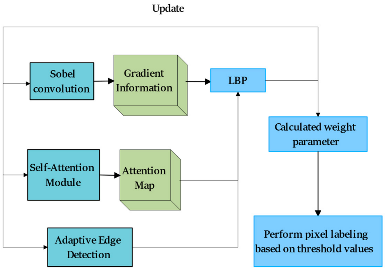
The fundamental principle of LAMBA is to adapt to different image features by comprehensively considering gradients, textures, and intensity. Unlike most self-attention mechanisms, in the initial stages of the task, we employ local binary pattern (LBP) features and adaptive edge detection to capture local texture and edge information, guiding the multi-head self-attention mechanism to focus on various directional information, thereby enhancing the model’s ability to extract coastlines. In LAMBA, the spatial information of pixels is leveraged to integrate multi-directional feature modules. The following section outlines the detailed steps Figure 4:
Initially, the input image undergoes prediction to generate the model’s output image. Let the prediction result be denoted as P   x ,   y , where x ,   y represents pixel coordinates. The Sobel convolution kernel is utilized to compute horizontal and vertical gradients, and the gradient information, along with the multi-head self-attention mechanism, is employed to adjust the projection direction.
x I x , y = Sobel x P x , y y I x , y = Sobel y P x , y
A i j = C o n c a t ( A t t e n t i o n 1 I , A t t e n t i o n 2 I , , A t t e n t i o n K I )
where Sobel x and Sobel y represent the Sobel convolution kernels, and A i j denotes the projection adjustment function.
Next, for each pixel, compute its local binary pattern (LBP):
L B P x , y = p = 0 P 1 s I p I x , y 2 p
where I p represents the grayscale value of the neighborhood points with the current pixel as the center, P is the number of neighborhood points, and s x is the step function.
Consider dynamically adjusting high and low thresholds based on local image properties and calculating the average intensity value within the local window.
W x , y = 1 N i = x W x x + W x j = y W y y + W y P i , j
T high x , y = k high a v g W x , y
T low x , y = k low a v g W x , y
Finally, we introduce weight parameters and combine LBP, adaptive edge detection, and self-attention mechanisms to compute comprehensive features.
F x , y = δ L B P x , y + γ a v g W x , y + 1 γ δ D A
D A I , A i j = α x I + 1 α A i j , β × y I + ( 1 β ) × A i j
where L B P x , y represents the LBP feature for each pixel, a v g W x , y is the average intensity value within the local window, DA I , A i j is the function obtained after adjusting the projection direction using gradient information and the multi-head self-attention mechanism, where α , δ , γ and β are weight parameters.
Perform pixel labeling based on the threshold values.
StrongEdge F x , y T high x , y PotentialEdge T low x , y F x , y < T high x , y NonEdge F x , y < T low x , y

2.5. Auxiliary Loss Function

For adaptive thresholds, the threshold is not static but is determined based on the local attributes of the image. Consequently, we have redesigned the auxiliary function. This involves the incorporation of edge information to further modify the Dice Loss. The underlying principle is that the edges or boundaries of objects within an image are particularly crucial in many segmentation tasks. By incorporating these boundaries into the loss function, the network can be directed toward generating enhanced segmentations, particularly along the edges of objects. The formulation is as follows:
L = L D + k × l E
L D is computed between the prediction and the ground truth.
l E represents the Dice Loss calculated between the predicted edge map (obtained through canny edge detection) and the ground truth.
k is a hyperparameter employed to determine the degree of emphasis on the edge Dice Loss within the final loss value.
In this paper, numerical stability is maintained by introducing the ‘smooth’ parameter. In instances where both the prediction and the ground truth lack discernible features, the Dice Loss may assume an indeterminate form of 0 / 0 . By adding a small “smooth” value to both the numerator and the denominator, such scenarios are circumvented, ensuring the stability of the loss value.
In summary, this enhanced Dice Loss leverages both global segmentation information and local edge details to yield superior segmentation outcomes, especially around object boundaries. Incorporating an edge-weighted term in the loss function is anticipated to guide the model to better handle boundaries and provide more accurate segmentation.

3. Experiment

3.1. Study Area

China, located in the southeastern part of the Asian continent, borders the Northwest Pacific Ocean. With nearly 3 million square kilometers of maritime territory and a coastline stretching over 32,000 km, China ranks sixth in the world. This coastline is bifurcated into mainland coastlines and island coastlines, with the former accounting for 18,000 km [56,57,58]. From 1980 to 2015, China’s coastline expanded by 3000 km. However, its natural coastline decreased by approximately 50% during the same period [57,59,60]. This transformation can be attributed to various factors, including monsoonal waves, tectonic uplift and subsidence, and human activities. Notably, the coastal regions, known for their rich resources and transportation convenience, accommodate only 40% of the country’s population but contribute 70% to China’s GDP, showcasing one of the most robust economic activities globally.
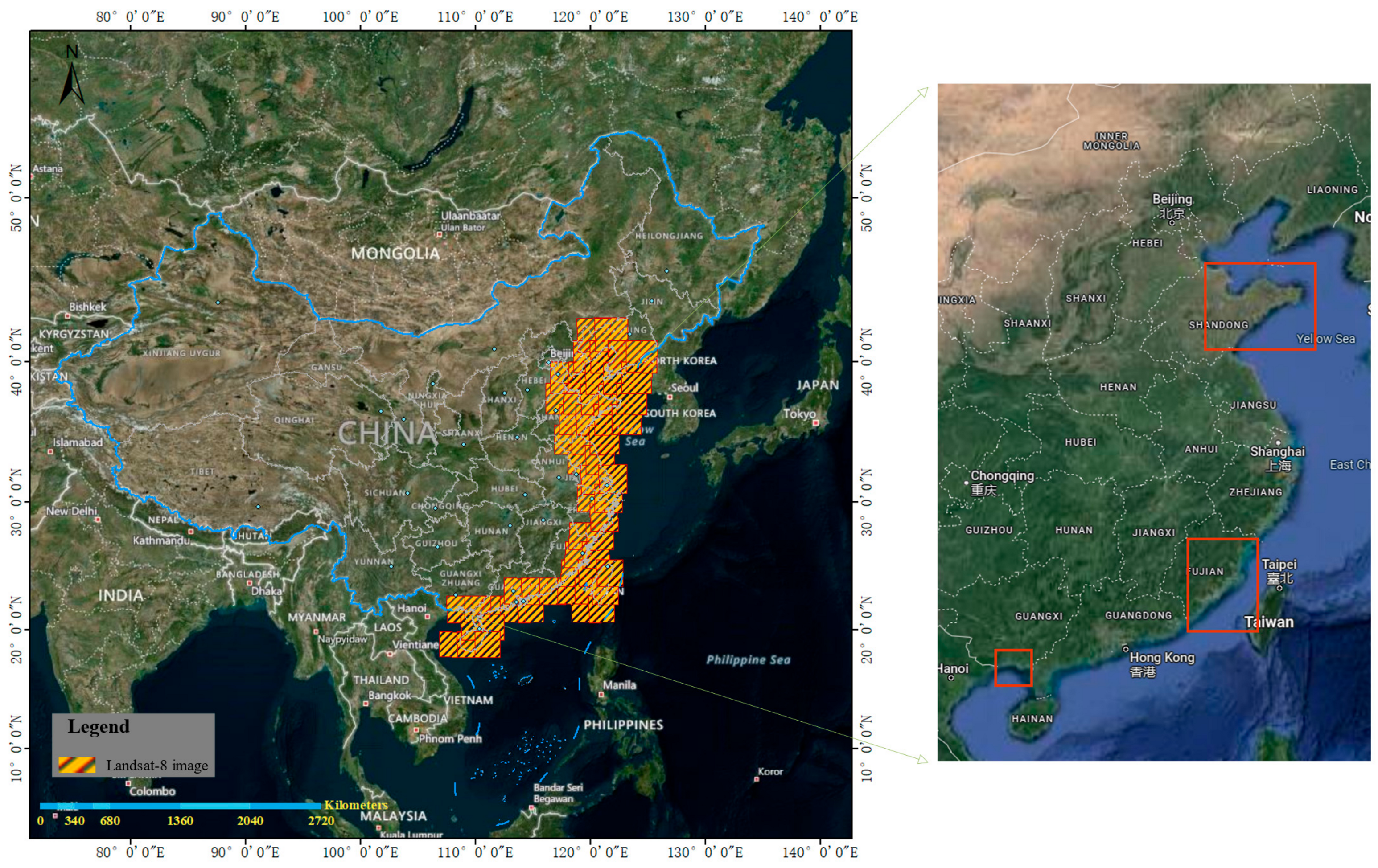
This study primarily examines the mainland coastline of China, as illustrated in Figure 5. The study area extends from the Yalu River Estuary in the north, situated on the China–North Korea border, to the Beilun Estuary in the south, which marks the China–Vietnam border. It encompasses four seas: the Bohai, Yellow, East, and South China Seas. It spans across 14 primary provinces, municipalities, and autonomous regions, cutting through three climatic zones: temperate, subtropical, and tropical. Based on geological and geomorphic features, coastlines can primarily be categorized into four types: sandy coasts, bedrock coasts, muddy coasts, and artificial coasts. From this, it is evident that China’s coastline is elongated and intricate, making extraction quite challenging.
Due to substantial topographical differences between northern and southern China, we chose datasets from Fujian Province, Guangxi Province, and Shandong Province to be the test set for evaluating our model’s generalizability comprehensively. The datasets from the other provinces were randomly divided into training and validation sets at a 4:1 ratio. The validation set adjusts model hyperparameters and monitors model performance during training. After each training epoch, the model is evaluated on the validation set to assess its ability to generalize to unseen data. The test set, consisting of data not encountered during training and validation, is used for the model’s final performance evaluation. It assesses the model’s ability to generalize to real-world data and evaluates the overall performance of the model. The experimental data in this study come from 103 multispectral images of the mainland China coastal zone captured by the “Landsat 8” satellite in 2020 [61,62].
After acquiring the images, various preprocessing steps were undertaken. These steps encompass orthorectification, image fusion, mosaicking, and cropping. A standard false-color composite image composed of Band 5, Band 4, and Band 3 was chosen for a more precise capture of coastline features. It was ensured that each selected image exhibited diverse coastline characteristics. Ground truth maps for land–sea segmentation of these images were created through expert visual interpretation. Following cropping of the preprocessed remote sensing images to create samples measuring 256 × 256 pixels, a total of 65,389 sample images were obtained. However, given the extensive scale of the data and the high costs associated with training, this study additionally employed a threshold method and expert visual recognition to filter out images containing solely a single landform feature. Within each remote sensing image, pixel values in the binary label map are set to 0 and 255. The threshold segmentation algorithm removes label maps with uniform gray values of 0 or 255, along with their original remote sensing images. Moreover, black borders in downloaded remote sensing images may misinterpret label images containing 0 and 255 gray values during screening, requiring manual scrutiny of the original image. Only images that concurrently showcased both land and sea features were retained. After this selection process, the final training set consisted of 4637 samples, the validation set contained 989 samples, and the test set had 1922 samples.

3.2. Coastline Dataset

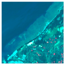
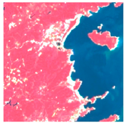
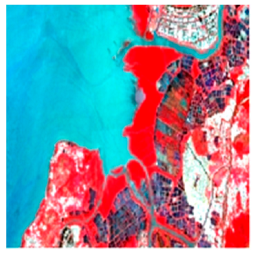
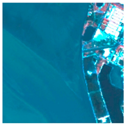
Extracting coastlines through deep learning necessitates the creation of precise remote-sensing image labels, constituting a pivotal step in the process. Ensuring accuracy in label creation is imperative for effectively enabling deep networks to discern terrain features during the training phase. In the past, when extracting coastlines from satellite remote sensing images, the instantaneous water boundary observed during satellite passes has frequently been regarded as the accurate coastline [63,64]. This differs significantly from the definition of the actual coastline as the sea–land boundary at the moment of the average high tide over several years. In order to objectively and accurately extract coastlines that closely resemble the actual coastline, this study utilizes the five coastal-type (Table 1) remote sensing interpretation markers proposed by Sun Weifu to construct a deep learning dataset [65].

3.3. Implementation Details

The experiments were conducted on a computer equipped with an NVIDIA RTX 3060 GPU with 12 GB of VRAM and running the Ubuntu 18 operating system. All models were trained and tested using the PyTorch framework. During the training process, the Adam optimizer was employed to minimize the loss. The initial learning rate was set to 1 × 10⁻³, with the number of iterations set at 100 epochs and a batch size of 8.

3.4. Evaluation Metrics

In this study, we utilize Intersection over Union (IoU), mean Intersection over Union (MioU), Frequency Weighted Intersection-over-Union (FWIoU), and Overall Accuracy (OA) to evaluate the performance of the model. These five evaluation metrics are derived from the confusion matrix, which comprises true positives (TP), false positives (FP), true negatives (TN), and false negatives (FN). Below are the computational formulas for each metric.
For each class, IoU is defined as the ratio of the intersection to the union of the predicted and true values. The formula is as follows:
I o U = T P T P + F P + F N
The MIoU represents the average result of the IoU for each class. Its calculation is given by:
M I o U = i n I o U n
FWIoU assigns weights based on the frequency of occurrences for each class. The weight is multiplied by the IoU for each class and then summed up. The formula for this is as follows:
F W I o U = T P + F N T P + F P + T N + F N × T P T P + F P + F N
The F1-Score (F1) takes into account both precision and recall, aiming for a balance that maximizes both. The formula for the F1 or each class is as follows:
  F 1 = 2 × p r e c i s i o n × r e c a l l p r e c i s i o n + r e c a l l
P r e c i s i o n = T P T P + F P
R e c a l l = T P T P + F N
Accuracy (ACC) indicates the proportion of correctly predicted samples among all samples. This includes both true positive and true negative predictions. The calculation for accuracy is as follows:
A c c u r a c y = T P + F N T P + F P + T N + F N

4. Results

4.1. Performance of Daenet

This paper contrasts the performance of DAENet with several existing methods, including Segmenter [66], Mask2Former [67], and Swin-UNet. All three methods are built upon the Transformer architecture. Specifically, Mask2Former is a hybrid structure based on Mask R-CNN and Transformer, while Swin-UNet constitutes a UNet structure formed purely from Swin Transformer modules. The three methods, PIDNet [68], DDRNet [69], and SegNeXt [70], are state-of-the-art models established based on CNN. This study will analyze the accuracy and adaptability of the DAENet model from two perspectives:
(1) Conducting an analysis using evaluation metrics and results to ascertain and validate its accuracy.
The results for the Shandong Province dataset are presented in Table 2, which showcases the numerical outcomes for each semantic segmentation method. The findings indicate that DAENet outperforms other techniques in metrics such as IoU, MIoU, FWIoU, and overall OA.
For the Mask2Former model, which has achieved SOTA results in semantic, instance, and panoptic segmentation as a unified segmentation structure, Table 2, Table 3 and Table 4 reveal its performance on coastline data extraction is not especially commendable. As a comprehensive, large-scale model designed to incorporate a wide array of features, it unavoidably sacrifices precision when isolating specific ones. Consequently, it loses its SOTA edge when extracting the requisite edge information for coastline detection.
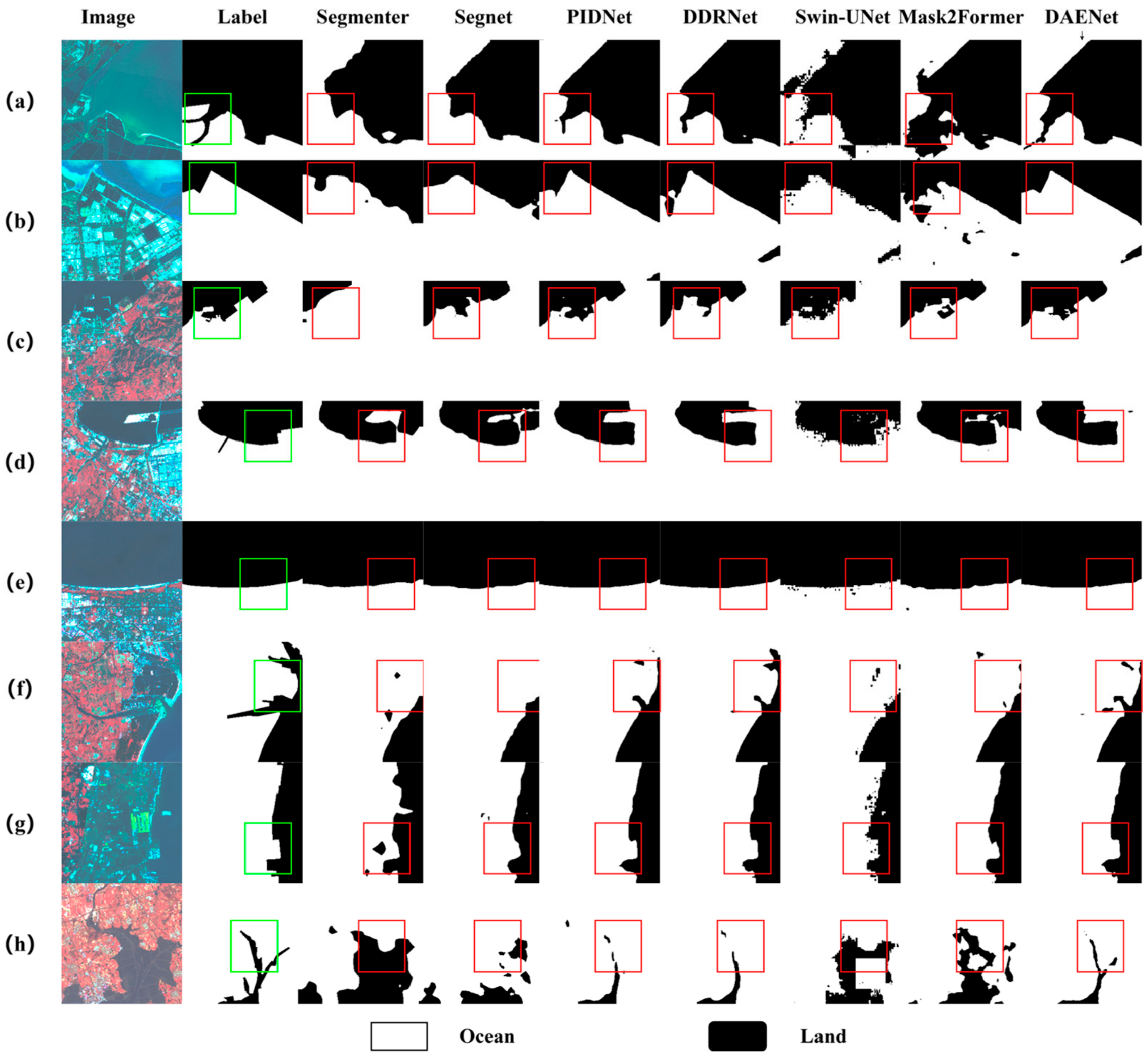
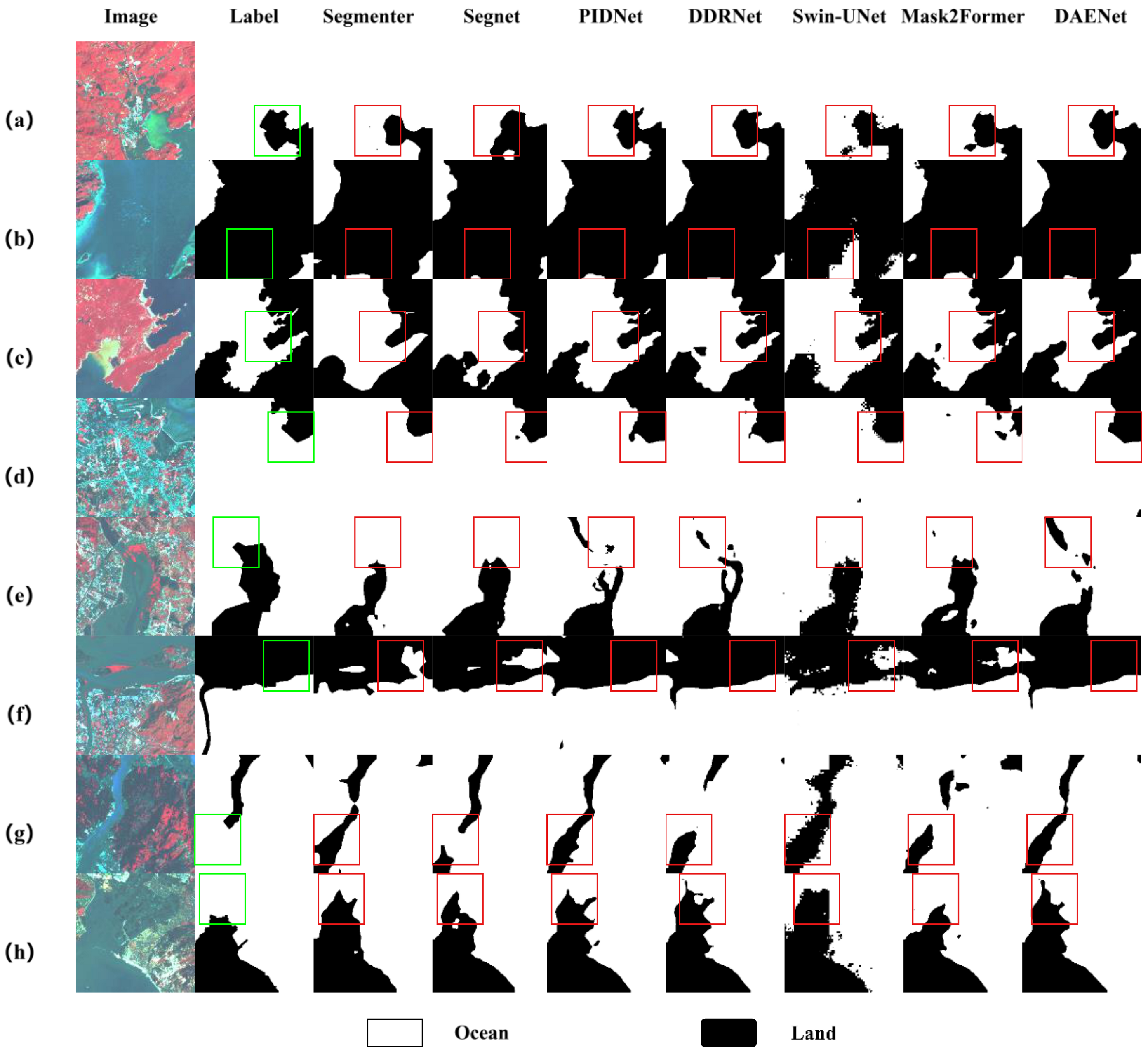
In reference to the Swin-UNet, predominantly employing the Swin Transformer module for semantic segmentation, the model, despite its superior global modeling capability, necessitates revision when configured according to the Swin-UNet design for remote sensing imagery [58]. This deficiency becomes apparent in Figure 6, Figure 7 and Figure 8, illustrating fragmented semantic segments in boundary extraction, a common issue stemming from ambiguity in edge information. However, upon integrating the LAMBA and MST modules into our DAENet, Figure 6, Figure 7 and Figure 8 demonstrate more accurate edge extraction and the absence of fragmented semantic segments, thereby reinforcing the model’s robustness in edge detection.
With regard to the straightforward, efficient, and durable semantic segmentation model, Segmenter, our assessments have indicated that its functionality is marginally inadequate. As depicted in Figure 6 (Segmenter. e), although it capably handles simple linear coastlines with minimal discrepancies, its proficiency significantly decreases when confronting complex feature patterns, as exemplified in sections a, f, and g of the same Figure 6, Figure 7 and Figure 8. In comparison, DAENet’s performance remains superior for dense and intricate terrestrial entities, as evident in Figure 6, Figure 7 and Figure 8.
(2) Conducting analysis across diverse regions to assess the adaptability of the model:
First, China’s coastlines can be primarily classified into three types based on geological and geomorphic characteristics: sandy coasts, bedrock coasts, and artificial coasts. As depicted in Figure 6b,c for artificial coasts and Figure 7 for sandy and bedrock coasts, the coastline morphologies extracted by our DAEnet demonstrate superior performance compared to other methods.
Secondly, we also analyzed results from other types of coastlines. During the generation of estuary labels, especially in manual labeling processes, if narrow rivers extend over a considerable distance, our usual approach involves capturing either a segment of the estuary shoreline or rectifying the shoreline directly. Nevertheless, when confronted with images containing incomplete labeling (see Figure 7h) or featuring coastlines marked by aquaculture ponds (see Figure 6a,h), as well as other complex coastal types, we are nonetheless able to accurately discern the correct shoreline.
Lastly, as illustrated in Figure 7, the coastline of Fujian Province is notably intricate, winding its way in an exceptionally complex manner, making it the most complex coastline in mainland China. Despite this challenging topography, our DAENet consistently performs at a high level, with all performance metrics exceeding 84%, establishing it as a leading method in the industry. Additionally, we predicted the coastline of Guangxi Province using the DAENet model, with extracted results demonstrating superior performance compared to other models, confirming the reliability of DAENet. With sufficient data, we will be fully equipped to extract coastlines from across the country and monitor their dynamic changes.

4.2. Ablation Study

To evaluate the performance of the proposed network architecture and its three crucial modules, we utilized UNet as the foundational network for conducting an ablation study on the dataset. Furthermore, we explored the impact of the loss function on the proposed network. The subsequent comparison results indicate that the integration of the proposed MST, LAMBA, and DAT modules yields significant performance enhancements in detection (Figure 9).
(1) Impact of the Deformable Self-Attention Module: As presented in Table 5, introducing the Deformable Attention Transformer (DAT) effectively augments the segmentation performance of the UNet structure. There is an improvement ranging from 5.69% to 6.45% in the IoU accuracy metric relative to the original baseline model. The enhancement in accuracy ranges from 9.42% to 10.28%, providing substantial evidence for the effectiveness of integrating DAT. This enhancement is attributed to the feature maps first undergoing processing via window-based local attention, facilitating local information aggregation. Subsequently, the Deformable Attention block models the global relationships among the locally enhanced tokens. This alternative attention block design, equipped with local and global receptive fields, aids the model’s learning process.
(2) The incorporation of the multi-scale transformation module (MST) into the Swin-UNet + LAMBA and Dat-UNet + LAMBA models yields significant results. As illustrated in Table 5, the integration of the multi-scale deformable edge detection module significantly enhances the segmentation performance of the UNet architecture. Relative to the original model, there is an improvement of 1.28% to 1.93% in the IoU accuracy metric. For the accuracy metric, the enhancement ranges from 1.01% to 1.72%. These outcomes underscore that integrating the MST module facilitates the model by capturing a richer set of feature information.
(3) Impact of the LAMBA Module: The LAMBA module was, respectively, integrated into the Swin-UNet and Dat-UNet models. As depicted in Table 5, the adaptive edge detection module’s introduction bolsters the segmentation performance of the UNet structure. Compared to the original model, there is a boost of 1.03% to 2.67% in the IoU accuracy metric. Regarding the accuracy metric, the uplift spans from 1.07% to 1.45%. These findings highlight that introducing the LAMBA module amplifies the model’s proficiency in edge delineation.

5. Conclusions

In this study, we propose DAENet, a deep learning model that combines semantic segmentation networks with edge detection to address inaccuracies in coastline extraction and localization. To enhance the model’s feature representation, we introduce the multi-scale transformation (MST) module, which incorporates canny edge detection across multiple spatial scales as input channels. By integrating MST into the U-shaped network structure, our model gains improved global modeling capability compared to traditional CNNs and patch-based Transformers. Additionally, our novel LAMBA module focuses on capturing edge features in the spatial dimension to mitigate semantic ambiguity caused by unclear object boundaries. We refine the binary Dice Loss function to expedite convergence and compute an edge-perceptive loss utilizing Canny edge maps to augment performance on edges further. Experimental results demonstrate that DAENet outperforms traditional models like Segmenter, SegNeX, PIDNet, DDRNet, Swin-UNet, and Mask2Former. Compared to the traditional model, Swin-UNet, DAENet shows a 5% improvement in MIoU.
To our knowledge, the proposed DAENet model is the first to apply the DAT block for remote sensing sea–land segmentation. It addresses the limitations of pure CNNs and enhances segmentation accuracy. The proposed network model can be effectively applied to precise positioning tasks for various complex coastal types in different regions, demonstrating its potential for coastal dynamic management and planning. Furthermore, the unique dataset created in this study allows the extracted results to approximate the actual coastline closely.
However, our model has several limitations. (1) DAENet extensively uses the Deformable Attention module, resulting in a larger parameter set and slightly longer training durations than other methods. This may limit DAENet’s use in compact mobile devices, but it still offers valuable insights into the roles of Deformable Attention in remote sensing semantic segmentation. In future research, we will design more accurate geometric prior models and loss functions for SLS segmentation features or generate multi-scale features through style transfer to accelerate model convergence. (2) DAENet still requires improvements in object boundary extraction. The deficiencies mainly appear in the segmentation results, where we aim to explore advanced encoding techniques for boundary features to overcome this limitation. Augmented outcomes deviate from the actual shape of the objects and show slight noise. Additionally, we will prioritize implementing model compression methods to enhance inference efficiency. Overall, the goal is to accelerate model convergence while retaining its deformable characteristics.

Author Contributions

Conceptualization, B.K. and J.X.; Methodology, B.K., J.W. and J.X.; Software, B.K.; Validation, B.K.; Formal analysis, J.W.; Investigation, B.K.; Data curation, B.K. and J.X.; Writing—original draft, B.K.; Writing—review & editing, J.W., J.X. and C.W.; Supervision, J.W. and C.W.; Project administration, J.X.; Funding acquisition, J.X. All authors have read and agreed to the published version of the manuscript.

Funding

This research was funded by the High-Resolution Remote Sensing Applications Demonstration System for Urban Fine Management of China (Grant number 06-Y30F04-9001-20/22) and the National Key R&D Program of China (Grant number 06-Y30F04-9001-20/22).

Institutional Review Board Statement

Not applicable.

Informed Consent Statement

Not applicable.

Data Availability Statement

The original contributions presented in the study are included in the article, further inquiries can be directed to the corresponding author.

Conflicts of Interest

The authors declare no conflicts of interest.

References

  1. Chen, C.; Bu, J.; Zhang, Y.; Zhuang, Y.; Chu, Y.; Hu, J.; Guo, B. The application of the tasseled cap transformation and feature knowledge for the extraction of coastline information from remote sensing images. Adv. Space Res. 2019, 64, 1780–1791. [Google Scholar] [CrossRef]
  2. Gens, R. Remote sensing of coastlines: Detection, extraction and monitoring. Int. J. Remote Sens. 2010, 31, 1819–1836. [Google Scholar] [CrossRef]
  3. Yang, Z.; Wang, L.; Sun, W.; Xu, W.; Tian, B.; Zhou, Y.; Yang, G.; Chen, C. A new adaptive remote sensing extraction algorithm for complex muddy coast waterline. Remote Sens. 2022, 14, 861. [Google Scholar] [CrossRef]
  4. Mimura, N. Sea-level rise caused by climate change and its implications for society. Proc. Jpn. Acad. 2013, 89, 281–301. [Google Scholar] [CrossRef]
  5. Small, C.; Nicholls, R.J. A global analysis of human settlement in coastal zones. J. Coast. Res. 2003, 19, 584–599. [Google Scholar]
  6. Bell, P.S.; Bird, C.O.; Plater, A.J. A temporal waterline approach to mapping intertidal areas using X-band marine radar. Coast. Eng. 2016, 107, 84–101. [Google Scholar] [CrossRef]
  7. Green, E.; Mumby, P.J.; Edwards, A.J.; Clark, C.D. A review of remote sensing for the assessment and management of tropical coastal resources. Coast. Manag. 1996, 24, 1–40. [Google Scholar] [CrossRef]
  8. Vassilakis, E.; Papadopoulou-Vrynioti, K. Quantification of deltaic coastal zone change based on multi-temporal high resolution earth observation techniques. ISPRS Int. J. Geo-Inf. 2014, 3, 18–28. [Google Scholar] [CrossRef]
  9. Zhang, Y.; Hou, X. Characteristics of coastline changes on Southeast Asia Islands from 2000 to 2015. Remote Sens. 2020, 12, 519. [Google Scholar] [CrossRef]
  10. Bera, R.; Mait, R. Quantitative analysis of erosion and accretion (1975–2017) using DSAS—A study on Indian Sundarbans. Reg. Stud. Mar. Sci. 2019, 28, 100583. [Google Scholar] [CrossRef]
  11. Ghosh, M.K.; Kumar, L.; Roy, C. Monitoring the coastline change of Hatiya Island in Bangladesh using remote sensing techniques. ISPRS J. Photogramm. Remote Sens. 2015, 101, 137–144. [Google Scholar] [CrossRef]
  12. Konko, Y.; Okhimambe, A.; Nimon, P.; Asaana, J.; Rudant, J.P.; Kokou, K. Coastline change modelling induced by climate change using geospatial techniques in Togo (West Africa). Adv. Remote Sens. 2020, 9, 85–100. [Google Scholar] [CrossRef]
  13. Hamylton, S.; Prosper, J. Development of a spatial data infrastructure for coastal management in the Amirante Islands. Int. J. Appl. Earth Obs. Geoinf. 2020, 19, 24–30. [Google Scholar] [CrossRef]
  14. Wu, G.; de Leeuw, J.; Skidmore, A.K.; Liu, Y.; Prins, H.H. Performance of Landsat TM in ship detection in turbid waters. Int. J. Appl. Earth Obs. Geoinf. 2012, 11, 54–61. [Google Scholar] [CrossRef]
  15. Giardino, C.; Bresciani, M.; Villa, P.; Martinelli, A. Application of remote sensing in water resource management: The case study of Lake Trasimeno, Italy. Water Resour. Manag. 2010, 24, 3885–3899. [Google Scholar] [CrossRef]
  16. Qiao, G.; Mi, H.; Wang, W.; Tong, X.; Li, Z.; Li, T.; Hong, Y. 55-year (1960–2015) spatiotemporal coastline change analysis using historical DISP and Landsat time series data in Shanghai. Int. J. Appl. Earth Obs. Geoinf. 2018, 68, 238–251. [Google Scholar]
  17. Sun, W.; Chen, C.; Liu, W.; Yang, G.; Meng, X.; Wang, L.; Ren, K. Coastline extraction using remote sensing: A review. GISci. Remote Sens. 2023, 60, 1780–1791. [Google Scholar] [CrossRef]
  18. Chen, C.; Qin, Q.; Zhang, N.; Li, J.; Chen, L.; Wang, J.; Yang, X. Extraction of bridges over water from high-resolution optical remote-sensing images based on mathematical morphology. Int. J. Remote Sens. 2014, 35, 3664–3682. [Google Scholar] [CrossRef]
  19. Chen, H.; Chen, C.; Zhang, Z.; Lu, C.; Wang, L.; He, X.; Chen, J. Changes of the spatial and temporal characteristics of land-use landscape patterns using multi-temporal Landsat satellite data: A case study of Zhoushan Island, China. Ocean. Coast. Manag. 2021, 213, 105842. [Google Scholar] [CrossRef]
  20. Elkhateeb, E.; Soliman, H.; Atwan, A.; Elmogy, M.; Kwak, K.S.; Mekky, N. A novel coarse-to-Fine Sea-land segmentation technique based on Superpixel fuzzy C-means clustering and modified Chan-Vese model. IEEE Access. 2021, 9, 53902–53919. [Google Scholar] [CrossRef]
  21. Tong, Q.; Shan, J.; Zhu, B.; Ge, X.; Sun, X.; Liu, Z. Object-Oriented Coastline Classification and Extraction from Remote Sensing Imagery. In Proceedings of the Remote Sensing of the Environment: 18th National Symposium on Remote Sensing of China, Beijing, China, 7–10 September 2007. [Google Scholar]
  22. Wang, P.; Zhuang, Y.; Chen, H.; Chen, L.; Shi, H.; Bi, F. Pyramid integral image reconstruction algorithm for infrared remote sensing sea-land segmentation. In Proceedings of the 2017 IEEE International Geoscience and Remote Sensing Symposium (IGARSS), Fort Worth, TX, USA, 23–28 July 2017; pp. 3763–3766. [Google Scholar]
  23. Wang, D.; Cui, X.; Xie, F.; Jiang, Z.; Shi, Z. Multi-feature sea–land segmentation based on pixel-wise learning for optical remote-sensing imagery. Int. J. Remote Sens. 2017, 38, 4327–4347. [Google Scholar] [CrossRef]
  24. Lei, S.; Zou, Z.; Liu, D.; Xia, Z.; Shi, Z. Sea-land segmentation for infrared remote sensing images based on superpixels and multi-scale features. Infrared Phys. Technol. 2018, 91, 12–17. [Google Scholar] [CrossRef]
  25. Chen, C.; Fu, J.; Zhang, S.; Zhao, X. Coastline information extraction based on the tasseled cap transformation of Landsat-8 OLI images. Estuar. Coast. Shelf Sci. 2019, 217, 281–291. [Google Scholar] [CrossRef]
  26. Chen, C.; Liang, J.; Xie, F.; Hu, Z.; Sun, W.; Yang, G.; Zhang, Z. Temporal and Spatial Variation of Coastline Using Remote Sensing Images for Zhoushan Archipelago, China. Int. J. Appl. Earth Obs. Geoinf. 2022, 107, 102711. [Google Scholar] [CrossRef]
  27. Fisher, P. The Pixel: A Snare and a Delusion. Int. J. Remote Sens. 1997, 18, 679–685. [Google Scholar] [CrossRef]
  28. Liu, Y.; Zhang, M.; Xu, P.; Guo, Z. SAR ship detection using sea-land segmentation-based convolutional neural network. In Proceedings of the 2017 International Workshop on Remote Sensing with Intelligent Processing (RSIP), Shanghai, China, 18–21 May 2017. [Google Scholar]
  29. Li, R.; Liu, W.; Yang, L.; Sun, S.; Hu, W.; Zhang, F.; Li, W. DeepUNet: A Deep Fully Convolutional Network for Pixel-level Sea-Land Segmentation. IEEE J. Sel. Top. Appl. Earth Obs. Remote Sens. 2018, 11, 3954–3962. [Google Scholar] [CrossRef]
  30. Lin, Z.; Ji, K.; Leng, X.; Kuang, G. Squeeze and excitation rank faster R-CNN for ship detection in SAR images. IEEE Trans. Geosci. Remote Sens. Lett. 2019, 16, 751–755. [Google Scholar] [CrossRef]
  31. Yang, T.; Jiang, S.; Hong, Z.; Zhang, Y.; Han, Y.; Zhou, R.; Kuc, T.Y. Sea-land segmentation using deep learning techniques for landsat-8 OLI imagery. Mar. Geod. 2020, 43, 105–133. [Google Scholar] [CrossRef]
  32. Hui, G.; Xiaodong, Y.; Heng, Z.; Yiting, N.; Jiaqi, W. Multi-scale sea-land segmentation method for remote sensing images based on Res2Net. Acta Optia Sin. 2022, 42, 1828004. [Google Scholar]
  33. Li, Y.; Wang, X.; Zhang, X.; Fang, J.; Zhang, X. WRBSNet: A Novel Sea–Land Segmentation Network With a Wider Range of Batch Sizes. IEEE Geosci. Remote Sens. Lett. 2024, 21, 1–5. [Google Scholar] [CrossRef]
  34. Chen, C.; Zou, Z.; Sun, W.; Yang, G.; Song, Y.; Liu, Z. Mapping the distribution and dynamics of coastal aquaculture ponds using Landsat time series data based on U2-Net deep learning model. Int. J. Digit. Earth 2024, 17, 2346258. [Google Scholar] [CrossRef]
  35. Ji, X.; Tang, L.; Lu, T.; Cai, C. DBENet: Dual-Branch Ensemble Network for Sea-Land Segmentation of Remote Sensing Images. IEEE Trans. Instrum. Meas. 2023, 72, 5503611. [Google Scholar] [CrossRef]
  36. Sun, S.; Mu, L.; Feng, R.; Chen, Y.; Han, W. Quadtree decomposition-based Deep learning method for multiscale coastline extraction with high-resolution remote sensing imagery. Sci. Remote Sens. 2024, 9, 100112. [Google Scholar] [CrossRef]
  37. Li, Z.; Cui, B.; Yang, G. Edge detection network model of coastline based on deep learning. Comput. Engin. Sci. 2022, 44, 2220–2229. [Google Scholar]
  38. Yu, F.; Koltun, V. Multi-scale context aggregation by dilated convolutions. arXiv 2015, arXiv:1511.07122. [Google Scholar]
  39. Dong, R.; Pan, X.; Li, F. DenseU-Net-Based Semantic Segmentation of Small Objects in Urban Remote Sensing Images. IEEE Access. 2019, 7, 65347–65356. [Google Scholar] [CrossRef]
  40. Chen, X.; Li, Z.; Jiang, J.; Han, Z.; Deng, S.; Li, Z.; Liu, M. Adaptive Effective Receptive Field Convolution for Semantic Segmentation of VHR Remote Sensing Images. IEEE Geosci. Remote Sens. 2021, 59, 3532–3546. [Google Scholar] [CrossRef]
  41. Ding, L.; Tang, H.; Bruzzone, L. LANet: Local Attention Embedding to Improve the Semantic Segmentation of Remote Sensing Images. IEEE Trans. Geosci. Remote Sens. 2021, 59, 426–435. [Google Scholar] [CrossRef]
  42. Yang, L.; Wang, X.; Zhai, J. Waterline Extraction for Artificial Coast With Vision Transformers. Front. Environ. Sci. 2022, 10, 799250. [Google Scholar] [CrossRef]
  43. Zheng, S.; Lu, J.; Zhao, H.; Zhu, X.; Luo, Z.; Wang, Y.; Fu, Y.; Feng, J.; Xiang, T.; Torr, P.H.S.; et al. Rethinking Semantic Segmentation from a Sequence-To-Sequence Perspective with Transformers. arXiv 2021, arXiv:2012.15840. [Google Scholar]
  44. Xie, E.; Wang, W.; Yu, Z.; Anandkumar, A.; Alvarez, J.M.; Luo, P. SegFormer: Simple and efficient design for semantic segmentation with transformers. Adv. Neural Inf. Process. Syst. 2021, 34, 12077–12090. [Google Scholar]
  45. Yang, Z.; Wang, G.; Feng, L.; Wang, Y.; Wang, G.; Liang, S. A Transformer Model for Coastline Prediction in Weitou Bay, China. Remote Sens. 2023, 15, 4771. [Google Scholar] [CrossRef]
  46. Zhu, Y.; Wang, B.; Liu, Q.; Tan, S.; Wang, S.; Ge, W. SRMA: A Dual-Branch Parallel Multi-Scale Attention Network for Remote Sensing Images Sea-Land Segmentation. Int. J. Remote Sens. 2024, 45, 3370–3395. [Google Scholar] [CrossRef]
  47. Han, K.; Wang, Y.; Chen, H.; Chen, X.; Guo, J.; Liu, Z.; Tang, Y.; Xiao, A.; Xu, C.; Xu, Y.; et al. A Survey on Vision Transformer. IEEE Trans. Pattern Anal. Mach. Intell. 2022, 45, 87–110. [Google Scholar] [CrossRef]
  48. Guo, J.; Han, K.; Wu, H.; Tang, Y.; Chen, X.; Wang, Y.; Xu, C. CMT: Convolutional Neural Networks Meet Vision Transformers. In Proceedings of the IEEE/CVF Conference on Computer Vision and Pattern Recognition, New Orleans, LA, USA, 18–24 June 2022; pp. 12175–12185. [Google Scholar]
  49. Guo, M.-H.; Xu, T.-X.; Liu, J.-J.; Liu, Z.-N.; Jiang, P.-T.; Mu, T.-J.; Zhang, S.-H.; Martin, R.R.; Cheng, M.-M.; Hu, S.-M. Attention Mechanisms in Computer Vision: A Survey. Comp. Vis. Media 2022, 8, 331–368. [Google Scholar] [CrossRef]
  50. Liu, Z.; Lin, Y.; Cao, Y.; Hu, H.; Wei, Y.; Zhang, Z.; Lin, S.; Guo, B. Swin Transformer: Hierarchical Vision Transformer using Shifted Windows. In Proceedings of the 2021 IEEE/CVF International Conference on Computer Vision (ICCV), Montreal, QC, Canada, 10–17 October 2021; pp. 9992–10002. [Google Scholar]
  51. Wang, W.; Xie, E.; Li, X.; Fan, D.-P.; Song, K.; Liang, D.; Lu, T.; Luo, P.; Shao, L. Pyramid Vision Transformer: A Versatile Backbone for Dense Prediction Without Convolutions. In Proceedings of the IEEE/CVF International Conference on Computer Vision, Montreal, QC, Canada, 10–17 October 2021. [Google Scholar]
  52. Dai, J.; Qi, H.; Xiong, Y.; Li, Y.; Zhang, G.; Hu, H.; Wei, Y. Deformable Convolutional Networks. In Proceedings of the IEEE International Conference on Computer Vision, Venice, Italy, 22–29 October 2017; pp. 764–773. [Google Scholar]
  53. Wang, Y.; Liu, W.; Sun, W.; Meng, X.; Yang, G.; Ren, K. A Progressive Feature Enhancement Deep Network for Large-Scale Remote Sensing Image Superresolution. IEEE Trans. Geosci. Remote Sens. 2023, 61, 5619413. [Google Scholar] [CrossRef]
  54. Li, X.; Xu, F.; Liu, F.; Tong, Y.; Lyu, X.; Zhou, J. Semantic Segmentation of Remote Sensing Images by Interactive Representation Refinement and Geometric Prior-Guided Inference. IEEE Trans. Geosci. Remote Sens. 2024, 62, 5400318. [Google Scholar] [CrossRef]
  55. Xia, Z.; Pan, X.; Song, S.; Li, L.E.; Huang, G. Vision Transformer with Deformable Attention. In Proceedings of the IEEE/CVF Conference on Computer Vision and Pattern Recognition, New Orleans, LA, USA, 18–24 June 2022; pp. 4784–4793. [Google Scholar]
  56. Hou, X.; Wu, T.; Hou, W.; Chen, Q.; Wang, Y.; Yu, L. Characteristics of coastline changes in mainland China since the early 1940s. Sci. China Earth Sci. 2016, 59, 1791–1802. [Google Scholar] [CrossRef]
  57. Wu, T.; Hou, X.; Xu, X. Spatio-temporal characteristics of the mainland coastline utilization degree over the last 70 years in China. Ocean. Coast. Manag. 2014, 98, 150–157. [Google Scholar] [CrossRef]
  58. He, X.; Zhou, Y.; Zhao, J.; Zhang, D.; Yao, R.; Xue, Y. Swin transformer embedding UNet for remote sensing image semantic segmentation. IEEE Trans. Geosci. Remote Sens. 2022, 60, 4408715. [Google Scholar] [CrossRef]
  59. Wang, X.; Liu, Y.; Ling, F.; Liu, Y.; Fang, F. Spatio-temporal change detection of Ningbo coastline using Landsat time-series images during 1976–2015. ISPRS Int. J. Geo-Inf. 2017, 6, 68. [Google Scholar] [CrossRef]
  60. Meyer, E.L.; Matzke, N.J.; Williams, S.J. Remote sensing of intertidal habitats predicts West Indian topsnail population expansion but reveals scale-dependent bias. J. Coast. Conserv. 2015, 19, 107–118. [Google Scholar] [CrossRef]
  61. Xu, J.; Zhang, Z.; Zhao, X.; Wen, Q.; Zuo, L.; Wang, X.; Yi, L. Spatial and temporal variations of coastlines in northern China (2000–2012). Int. J. Geogr. Inf. Sci. 2013, 24, 18–32. [Google Scholar] [CrossRef]
  62. Guo, H. Big Earth data in support of the sustainable development goals (2019). Bull. Chin. Acad. Sci. 2021, 36, 932–939. [Google Scholar]
  63. Seale, C.; Redfern, T.; Chatfield, P.; Luo, C.; Dempsey, K. Coastline detection in satellite imagery: A deep learning approach on new benchmark data. Remote Sens. Environ. 2022, 278, 113044. [Google Scholar] [CrossRef]
  64. Zou, Z.; Chen, C.; Liu, Z.; Zhang, Z.; Liang, J.; Chen, H.; Wang, L. Extraction of aquaculture ponds along coastal region using u2-net deep learning model from remote sensing images. Remote Sens. 2022, 14, 4001. [Google Scholar] [CrossRef]
  65. Sun, W.F.; Ma, Y.; Zhang, J.; Liu, S.W.; Ren, G.B. Study of remote sensing interpretation keys and extraction technique of different types of shoreline. Bull. Surv. Mapp. 2011, 3, 41–44. [Google Scholar]
  66. Strudel, R.; Garcia, R.; Laptev, I.; Schmid, C. Segmenter: Transformer for semantic segmentation. In Proceedings of the IEEE/CVF International Conference on Computer Vision, Electrical Network, Montreal, BC, Canada, 11–17 October 2021; pp. 7262–7272. [Google Scholar]
  67. Guo, M.H.; Lu, C.Z.; Hou, Q.; Liu, Z.; Cheng, M.M.; Hu, S.M. Segnext: Rethinking convolutional attention design for semantic segmentation. arXiv 2022, arXiv:2209.08575. [Google Scholar]
  68. Xu, J.; Xiong, Z.; Bhattacharyya, S.P. PIDNet: A Real-Time Semantic Segmentation Network Inspired by PID Controllers. In Proceedings of the IEEE/CVF Conference on Computer Vision and Pattern Recognition, Vancouver, BC, Canada, 17–24 June 2023; pp. 19529–19539. [Google Scholar]
  69. Hong, Y.; Pan, H.; Sun, W.; Jia, Y. Deep dual-resolution networks for real-time and accurate semantic segmentation of road scenes. arXiv 2021, arXiv:2101.06085. [Google Scholar]
  70. Cheng, B.; Misra, I.; Schwing, A.G.; Kirillov, A.; Girdhar, R. Masked-attention mask transformer for universal image segmentation. In Proceedings of the IEEE/CVF Conference on Computer Vision and Pattern Recognition, New Orleans, LA, USA, 18–24 June 2022; pp. 1290–1299. [Google Scholar]
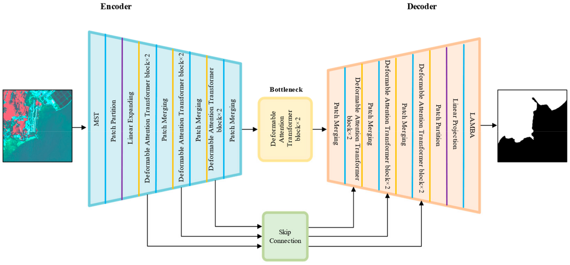
Figure 1. DAENet network structure.
Remotesensing 16 02076 g001
Figure 2. Multi-scale transformation module.
Remotesensing 16 02076 g002
Figure 3. An illustration of our Deformable Attention mechanism. (a) presents the information flow of Deformable Attention. In the left part, a group of reference points is placed uniformly on the feature map, whose offsets are learned from the queries by the offset network. Then, the deformed keys and values are projected from the sampled features according to the deformed points, as shown in the right part. Relative position bias is also computed by the deformed points, enhancing the multi-head attention, which outputs the transformed features. We show only four reference points for a clear presentation; there are many more points in real implementation de facto. (b) Reveals the detailed structure of the offset generation network, marked with sizes of feature maps.
Remotesensing 16 02076 g003
Figure 4. Local Adaptive Multi-Head Attention-based Edge Detection Module.
Remotesensing 16 02076 g004
Figure 5. Study area of China and its adjacent maritime regions.
Remotesensing 16 02076 g005
Figure 6. Examples of semantic segmentation results on the Shandong Province dataset. (ad,fh) artificial coastline; (e) sandy coastline.
Remotesensing 16 02076 g006
Figure 7. Examples of semantic segmentation results on the Fujian Province dataset. (a,g) artificial coastline & bedrock coastline; (b) bedrock coastline; (c) bedrock coastline & sandy coastline; (e) artificial coastline & biogenic coastline; (d,f,h) artificial coastline.
Remotesensing 16 02076 g007
Figure 8. Examples of semantic segmentation results on the Guangxi Province dataset. (a,b) silty coastline; (c,d) artificial coastline & silty coastline; (eh) artificial coastline.
Remotesensing 16 02076 g008
Figure 9. Examples of semantic segmentation results on the Ablation experiment: (a) Image, (b) U-Net, (c) Swin-UNet, (d) Dat-UNet, (e) Dat-UNet + MST, and (f) Dat-UNet + MST + LAMBA.
Remotesensing 16 02076 g009
Table 1. Five types of coastline.
CoastlineSampleInterpretation SignsLocation
Bedrock CoastlineRemotesensing 16 02076 i001Distinct concave-convex and mountainous texture featuresThe evident land–water boundary
Silty CoastlineRemotesensing 16 02076 i002Appears grey or white with a smooth textureA boundary that is located in an estuary, delta, or low-lying area and has a marked contrast in vegetation density
Sandy CoastlineRemotesensing 16 02076 i003Clear dividing line between white and other colorsBeach ridges and lack of beach ridges, the beach is directly adjacent to the cliffs of the bedrock shoreline
Biogenic CoastlineRemotesensing 16 02076 i004Red tones, darker textures, and irregular shapesIt is mainly distributed in Guangdong, Guangxi, Fujian, Taiwan, and parts of Hainan Island
Artificial CoastlineRemotesensing 16 02076 i005Bright and white structures, smooth textures and narrow stretches, regular layouts, and colors ranging from light beige to tan or even whiteA man-made coastline exhibits a multitude of features, which are often intricate and require thorough analysis and consideration
Table 2. Comparison of segmentation accuracy on the Shandong Province dataset.
MethodIoU(%)F1 (%)Evaluation Index
OceanLandOceanLandMioU (%)OA (%)FWIoU (%)
Segmenter90.4994.0992.2892.2185.6192.2585.61
SegNeXt95.6793.8494.7194.7790.0194.7490.01
PIDNet91.7492.0695.6995.8691.9095.7891.90
DDRNet92.1892.4895.9396.0992.3396.6692.33
Swin-UNet88.5988.3393.9593.8088.4693.8888.46
Mask2Former88.5388.4493.9193.8688.4893.8988.48
DAENet93.8594.0496.8296.9393.9496.8893.94
Table 3. Comparison of segmentation accuracy on the Fujian Province dataset.
MethodIoU (%)F1 (%)Evaluation Index
OceanLandOceanLandMioU (%)OA (%)FWIoU (%)
Segmenter82.0384.2089.9091.1683.1290.8283.16
SegNeXt83.7185.6491.1392.2684.6891.1384.72
PIDNet84.9986.8991.8892.9885.9492.4785.97
DDRNet85.4387.3092.1493.2286.3793.5386.40
Swin-UNet83.2285.2990.8492.0684.2591.4983.30
Mask2Former82.0884.6890.1691.7083.3891.0083.44
DAENet87.2888.8493.2094.0988.0693.6888.09
Table 4. Comparison of segmentation accuracy on the Guangxi Province dataset.
MethodIoU (%)F1 (%)Evaluation Index
OceanLandOceanLandMioU (%)OA (%)FWIoU (%)
Segmenter69.2877.9081.8587.5873.5985.2574.28
SegNeXt69.7077.8882.1487.5673.7985.3474.45
PIDNet72.0381.6383.7489.8877.6887.5377.68
DDRNet72.7282.0284.2090.1277.3787.8478.16
Swin-UNet74.5482.8885.4190.6378.7188.5979.38
Mask2Former71.2081.2183.1889.6376.2187.1777.01
DAENet76.3984.9186.6191.8480.6589.8681.33
Table 5. Comparison of ablation results.
MethodIoU (%) F 1
OceanLandOceanLand
U-Net83.2183.8790.8491.23
Swin-UNet88.5988.3393.9593.80
Swin-UNet + LAMBA88.9388.6594.1493.98
Swin-UNet + MST89.1689.3494.1194.01
Swin-UNet + LAMBA + MST90.2190.1494.8594.81
Dat-UNet89.6689.7694.5594.60
Dat-UNet + LAMBA92.3392.4196.0196.06
Dat-UNet + MST92.8992.4295.9896.04
Dat-UNet + LAMBA + MST93.8594.0496.8296.93
Disclaimer/Publisher’s Note: The statements, opinions and data contained in all publications are solely those of the individual author(s) and contributor(s) and not of MDPI and/or the editor(s). MDPI and/or the editor(s) disclaim responsibility for any injury to people or property resulting from any ideas, methods, instructions or products referred to in the content.