Article

Modeling the Effect of Vegetation Coverage on Unmanned Aerial Vehicles-Based Object Detection: A Study in the Minefield Environment

by
Jasper Baur
1,2,*,
Kyle Dewey
1,
Gabriel Steinberg
1 and
Frank O. Nitsche
2
1
Demining Research Community, New York, NY 10027, USA
2
Lamont Doherty Earth Observatory, Columbia University, New York, NY 10027, USA
*
Author to whom correspondence should be addressed.
Remote Sens. 2024, 16(12), 2046; https://doi.org/10.3390/rs16122046
Submission received: 19 April 2024 / Revised: 21 May 2024 / Accepted: 5 June 2024 / Published: 7 June 2024

Abstract

:
An important consideration for UAV-based (unmanned aerial vehicle) object detection in the natural environment is vegetation height and foliar cover, which can visually obscure the items a machine learning model is trained to detect. Hence, the accuracy of aerial detection of objects such as surface landmines and UXO (unexploded ordnance) is highly dependent on the height and density of vegetation in a given area. In this study, we develop a model that estimates the detection accuracy (recall) of a YOLOv8 object’s detection implementation as a function of occlusion due to vegetation coverage. To solve this function, we developed an algorithm to extract vegetation height and coverage of the UAV imagery from a digital surface model generated using structure-from-motion (SfM) photogrammetry. We find the relationship between recall and percent occlusion is well modeled by a sigmoid function using the PFM-1 landmine test case. Applying the sigmoid recall-occlusion relationship in conjunction with our vegetation cover algorithm to solve for percent occlusion, we mapped the uncertainty in detection rate due to vegetation in UAV-based SfM orthomosaics in eight different minefield environments. This methodology and model have significant implications for determining the optimal location and time of year for UAV-based object detection tasks and quantifying the uncertainty of deep learning object detection models in the natural environment.

Graphical Abstract

1. Introduction

1.1. UAV-Based Object Detection

Object detection is a common computer vision task aimed at automating the identification and localization of various objects from imagery. Early deep object detection models faced the same limitations as other deep learning architectures—they were principally constrained by a lack of available computation and training data. This changed with the increased availability of cheap computational resources and the release of benchmark datasets like ImageNet [1]. ImageNet provided a benchmark through which various computer vision models were tested against one another. Convolutional neural networks (CNNs) earned wider recognition for detection tasks in 2012 with the introduction of AlexNet. CNNs started outperforming other architectures and showed the utility of deeper models for object detection [2]. Since then, CNNs have become the state-of-the-art for object detection, with some popular model architectures, including You Only Look Once (YOLO), Regional Convolutional Neural Networks (RCNN, Faster-RCNN), and Single Shot Detectors (SSD) [3,4,5,6].
The emergence of affordable UAS/V (unmanned aerial systems/vehicles), commonly known as drones, paired with the miniaturization of sensors has revolutionized the field of remote sensing, enabling critical progress in a diversity of applications from agriculture to earth science to mapping and emergency response [7,8,9]. UAVs equipped with visual, thermal, multispectral, magnetic, LiDAR, and other sensors are now commonplace in an industry that is expected to grow to over USD50 billion by 2050 [10]. Although a wide range of UAV-based sensors are available and in use across many sectors, by far, the most common is the visual light camera. Combining UAV-based visual cameras with Structure-from-Motion (SfM) photogrammetry allows for imagery to be processed into high-resolution 3D models of the environment that are difficult and expensive to obtain from traditional ground- or satellite-based techniques [11].
Along with most machine learning applications, UAV-based object detection is a rapidly maturing field with recently published benchmarked datasets such as Vis-Drone and hundreds of novel applications [12,13,14,15,16,17]. One application is the detection of landmines and other UXOs using convolutional neural networks (CNN) [18,19,20,21]. UAV-based CNNs for landmine and explosive remnants of war (ERW) detection improve the safety, time, and cost of clearing a minefield by providing situational awareness of where contamination is located and constraining suspected hazardous areas to smaller confirmed hazardous areas, all before a deminer steps foot into a contaminated field [22].

1.2. The Effect of Vegetation and Occlusion on Object Detection

Foliar cover, defined as the area above the soil covered by the vertical projection of exposed leaf area (or more simply, the shadow cast from a plant if the sun is directly above it) [23], presents a major limitation for UAV-based object detection in vegetated environments. The uncertainty due to vegetation and regolith cover evolves as seasons change and varies greatly from region to region. In most natural landscapes, vegetation growth will be the primary cause for surface-lain objects to become visually obscured from above. Different types of vegetation will result in a range of occlusion patterns that may influence an object detection model. For example, a few large, round leaves can occlude a large, continuous part of an object’s top surface, while thin blades of grass will occlude thin transects above the object. Additionally, occlusion patterns within the same species and same location can vary with leaf motion. In a desert environment, aeolian processes will be the dominant factor that leads to objects becoming visually obscured due to burial by dust and sand [24]. In coastal environments, a combination of coastal and hydrological processes, aeolian transport, and seasonal vegetation are all relevant for surface object detection. In the arctic, snow and ice are the primary factors that cause exposed objects to become visually obscured [25].
Previous studies addressing the challenge of occlusion for object detection tasks have predominantly come out of interest in self-driving cars, including applications for traffic sign, pedestrian, and car detection [26,27]. There have been a few attempts to quantify the effects on the recall of detection models of vegetation as a source of occlusion. This is because understanding the relationship between different variables within the occlusion context and the latent representation of the object within the model is extremely complex. To the authors knowledge, this is the first study that deals with quantifying how vegetation-based occlusion from UAV nadir (non-oblique) imagery affects recall.

1.3. Landmines and Cluster Munitions

Landmines and cluster munitions are dispersed in war to act as an area denial method for militaries and guerilla groups. During and after the conflict, these mines and munitions adversely affect communities by prohibiting land use, suppressing economic development and freedom of movement, and causing environmental degradation. There are millions of remnant unexploded ordnance (UXO), landmines, cluster munitions, and improvised explosive devices (IEDs), collectively referred to as EO (explosive ordnance), spanning 60 countries and regions [28]. Often, these EO are found in difficult terrains such as dense vegetation, steep slopes, and remote regions, leading to further logistical difficulties in the detection and clearance of these items [29]. The detection and clearance of EO are further exacerbated since landmine contamination prevents human land usage, leading to vegetation growth in these untouched areas, which in turn leads to higher foliar occlusion of surface-laid mines and increased difficulty of detection and clearance.
This widespread modern-day humanitarian crisis has caused on average 6540 ± 1900 injuries or deaths per year in the last two decades, with approximately 80% of the victims being civilians [28,30]. Casualties from mines are rising due to the February 2022 invasion in Ukraine, which has exacerbated this crisis, with studies citing up to 30% of the country as estimated to be contaminated by UXO and mines [31].
Cluster munitions are aerially dispersed bomblets that are dropped hundreds at a time and are currently being widely used in Ukraine. These munitions have inflicted nearly 1200 casualties in Azerbaijan, Iraq, Lao PDR, Lebanon, Myanmar, Syria, Ukraine, and Yemen in 2022, with children making up 71% of the victims [32]. While these munitions are intended to detonate on impact, detonation failure rates as high as 40% (but usually lower) result in thousands of volatile cluster munitions scattered over a large area of land [33]. Employing UAV-based deep learning models trained to detect surface cluster munitions is a promising method to combat these explosive hazards on a regional scale, but it currently lacks the ability to quantify detection rates in different environmental contexts with various degrees of vegetation.
Besides vegetation, other major challenges for detection of surface landmines and UXO include collecting imagery at high enough spatial resolution to resolve small anti-personnel mines, false positives from non-explosive debris, difficulty in attaining permissions and flying UAVs in electronic warfare environments close to conflict zones, collecting real-world training data for object detection models, and balancing the costs and complexities of integrating multi-sensor payloads to increase detection rates. Despite the challenges, great strides are being made in the field of humanitarian mine action to overcome these challenges and detect landmines using remote sensing around the world.

1.4. Motivation

Potentially, the most important consideration for UAV-based object detection accuracy in the natural environment is the vegetation of an area, which may visually obscure the items of interest (Figure 1). Hence, the accuracy of aerial detection of surface EO and other objects is highly dependent on the height and density of vegetation in a given area. Modeling prediction uncertainty is crucial for putting mine location predictions into context. For instance, if a model detects 75% of all objects within a designated field, it might imply that it detects 95% of the objects in the sparsely vegetated part of the field, yet only detects 55% of the objects in the more densely vegetated part of the field. It is, therefore, essential to quantify detection uncertainty in order to improve situational awareness about which areas are likely to have false negatives due to vegetation obscuring the view of the mines from above. While standard accuracy evaluation metrics such as global precision and recall are useful for determining average detection rates for deep learning object detection models, there is high variance between detection rates in different environments and vegetation.
To address this problem, we developed a model that uses the original UAV survey imagery to create detection rate maps for UAV-based object detection based on the foliar cover and the height of the object.

2. Materials and Methods

2.1. The Recall—Vegetated Occlusion Relationship

To determine the detectability of an object in a vegetated area from optical UAV imagery, we start by assuming the object is being viewed from above (nadir). We assume the object has a flat top surface with a height of Ho, and is visually distinct from the background environment (it is not camouflaged). This object is lying in a field where the maximum vegetation height is Hv (Figure 1). Note that vegetation assemblages in the real world have a myriad of complexities not depicted in Figure 1, such as diverse leaf patterns, differing growth stages, intergrowth of different species, overlapping leaves/canopy, and other morphological heterogeneities [34,35,36]. Additionally, topographical complexities on small and large scales, such as slopes, geomorphological features, craters, mounds, and holes, can influence the angle at which vegetation grows, which, in turn, influences whether an object is visible from a nadir view.
In the case where the object height is greater than the maximum vegetation height (Ho > Hv), foliar cover will have no effect on the detectability of the object. In this case, the detection rate will only rely on the object detection model recall.
Recall determines the percent of items of interest that are detected and is defined as follows:
R e c a l l = T P T P + F N
It is the number of true positives (TP, correct predictions) divided by the total number of validated reference items (TP + FN, false negatives). Precision is defined as the number of true positives divided by the number of true positives plus false positives, as follows:
P r e c i s i o n = T P T P + F P
It expresses the percentage of the predictions that match the validated reference data.
Conversely, if the object is fully obscured by vegetation (100% foliar cover), then the detection rate is theoretically 0%. In this situation, we define foliar cover (Fcover) as the percentage area where Hv > Ho in a unit area.
To solve the detection rate due to vegetation uncertainty using remotely sensed imagery, we must extract vegetation height and foliar coverage from the imagery and define the height of the object. We define “detectability” of a surface-lain object in vegetation viewed from above as follows:
D e t e c t a b i l i t y = R e c a l l ( F c o v e r )
where recall is a function of Fcover.
We isolate the effect of vegetation on detection rate by quantifying the uncertainty due to foliar cover through:
U n c e r t i a n t y   d u e   t o   f o l i a r   c o v e r = R e c a l l ( F c o v e r = 0 ) R e c a l l ( F c o v e r )

2.2. Synthetic Vegetation Growth

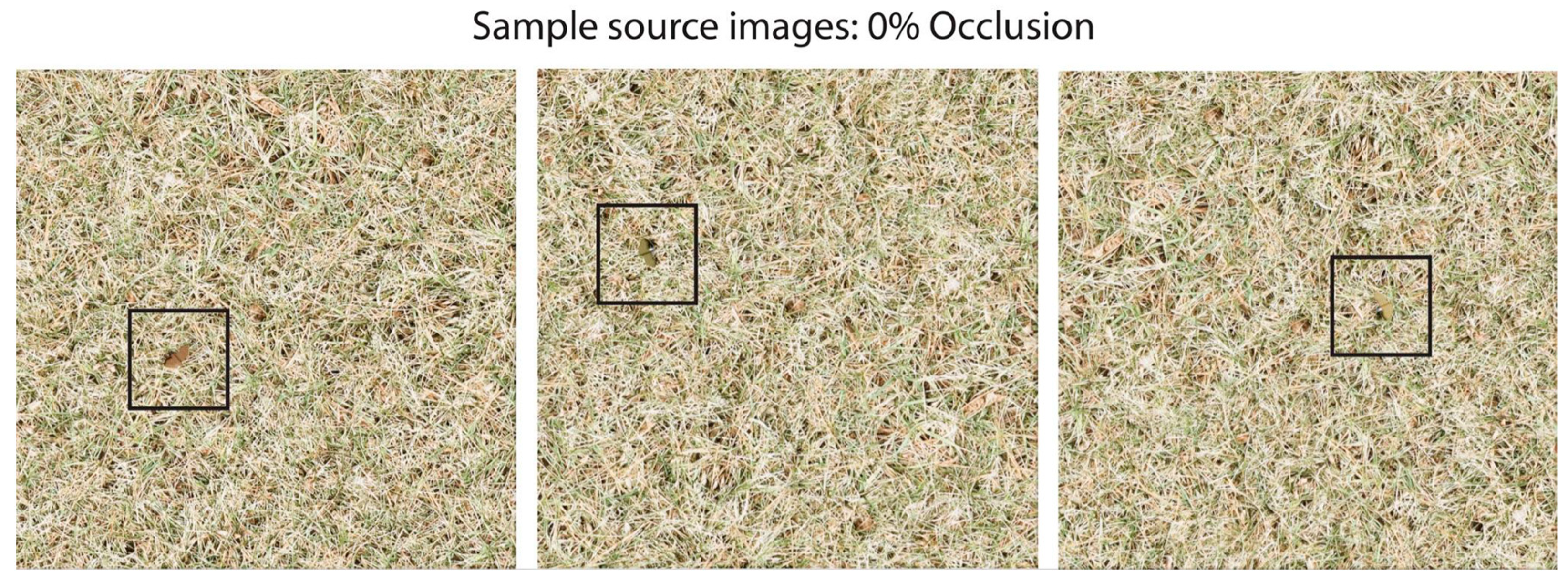
We utilize synthetic imagery to artificially “grow” grass over a mine, simulating natural occlusion due to vegetation growth, to solve the recall of the object detection model as a function of foliar cover (percent occlusion). The base synthetic images were created using NVIDIA Omniverse and 3D models of a PFM-1 landmine. From the placement of the 3D models, we also created a pixel mask (semantic segmentation mask) around the mines and a bounding box constraining the mine from the top left pixel to the bottom right pixel of the 3D model. (Figure 2). The PFM-1 is an anti-personnel mine about the size of a typical human hand, with dimensions of 11.9 cm × 6.4 cm × 2 cm and a weight of 75 g. The base images were then input into a vegetation growth simulation to programmatically add occlusion due to vegetation growth (Figure 3).
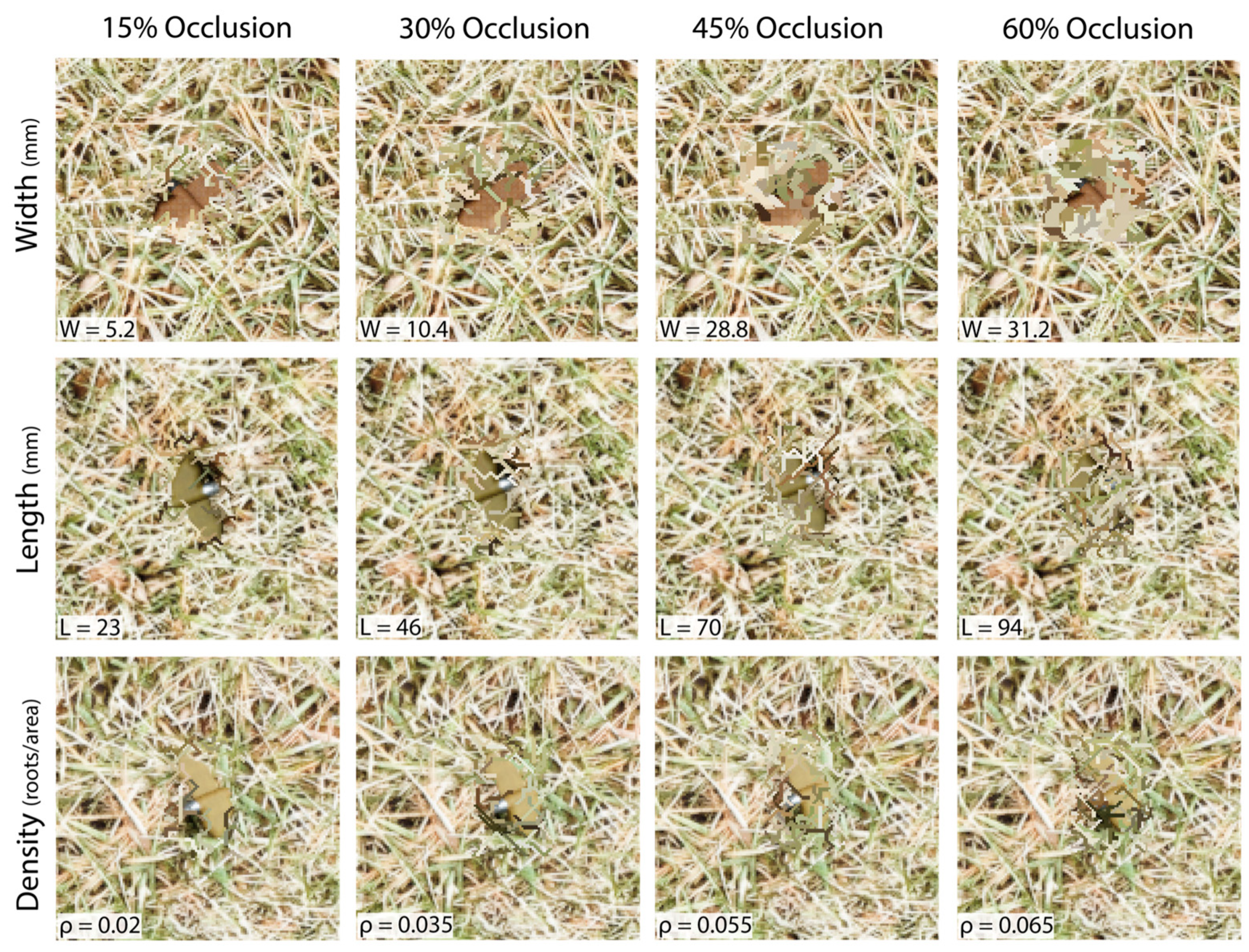
We simulated vegetation growth by expanding the bounding box around the mine by 50% along each axis and selecting a random pixel within the new bounding box that is not part of the semantic segmentation of the PFM-1. This pixel then becomes the “root” from which a blade of grass grows procedurally in a random direction. Once this process is repeated multiple times, it produces an effect that occludes areas on the edges of the mine first and those toward the center later, similarly to how grass occludes mines in the real world. To test the distinct factors that interplay in the natural environment, the simulation environment was designed to be able to vary the density, width, and length of the synthetic grass occlusion. The length variable is defined as the length of each grass blade in pixels. Width is increased by adding a given number of pixels below each pixel in the individual grass blade. For instance, if the thickness parameter is set to 3, an additional 2 pixels below each pixel in the blade are changed to the blade color. Density is a function of how many “roots” are generated inside the bounding box. This is represented as a ratio of the number of root pixels divided by the total number of pixels in the bounding box. Two simplifications that differ from the real world for the synthetic grass growth is that it assumes vegetation growth as a monoculture with constant height and density, and it does not produce shadows.
To generate a set of synthetic images, a user must specify the number of images to generate and an array of values for each of the three adjustable parameters. To solve recall as a function of occlusion, we generated 7930 synthetic-grass images (spanning a range of increasing grass density, widths, and lengths for 9 base images). Additionally, to independently test the effect of length, width, and density on occlusion detectability, we generated three synthetic datasets that isolated each variable with an average of 3250 synthetic images generated for each test.
Recall (Fcover) is an empirically derived function that calculates the recall for a specific object detection model with different degrees of occlusion. We generated a dataset of synthetic images with various amounts of grass occlusion and ran this dataset through a YOLOv8 convolutional neural network [37] trained to detect the PFM-1 landmine to determine the recall function. It is important to note that the neural network was not trained on any of the synthetic imagery. The synthetic dataset was used solely to assess the accuracy of a pre-trained neural network with varying degrees of validated vegetation cover. The PFM-1 model was trained from labeled UAV-produced orthomosaics of inert landmines. More details about how the PFM-1 neural network model was trained can be found in Baur et al.’s study in 2020 [18]. We calculated the detection rate or recall by binning all of the images for each percent occlusion and taking the mean of the binary result (either 1 or 0). For 0–80% occlusion, there was an average count of 100 data points per occlusion percentage (Figure S1).

2.3. Extracting Vegetation Height and Cover from UAV Imagery

In this section, we devise a method using imagery data from a UAV survey to estimate vegetation height (Hv) and foliar cover (Fcover)) to solve Equation (3). First, we process the UAV imagery using structure-from-motion photogrammetry. SfM photogrammetry involves computing the 3D structure of a scene from a sequence of overlapping photos created with a moving camera. The SfM algorithm first identifies distinct keypoints in each image and then matches these keypoints found in the overlapping images [11]. Based on the images and tie points (keypoint matches), the camera pose and parameters are computed, which are then used to reconstruct a dense point cloud. From the dense cloud, a 3D triangulation mesh and a digital surface model (DSM) surface can be computed. A DSM is an elevation model that represents the uppermost surface above the terrain (including natural and artificial features such as vegetation and buildings), and a digital terrain model (DTM) is an elevation model of the bare earth. An orthomosaic (a georeferenced imagery map) can also be computed by extrapolating the 2D image textures and colors onto the mesh surface. Due to the accessibility, cost effectiveness, and utility of SfM photogrammetry, it has been applied in a wide range of remote sensing applications, including geological mapping, forestry, agriculture, and hazard response [11,38,39].
We input the grid style UAV survey into Pix4DMapper version 4.8.4, a commercial photogrammetry software. We used the 3D-Maps template with the following default processing parameters—Keypoint image scale: Full, Matching Image Pairs: Aerial Gird or Corridor, Targeted Number of Keypoints: Automatic, Point Cloud Densification (Image Scale: ½, Point Density: Optimal, Minimum Number of Matches: 3). The processing workflow is optimized for UAV-based object detection on an orthomosaic since that is the context in which this imagery is collected, as opposed to generating the highest quality 3D models. In order for the imagery to be processed into an orthomosaic and DSM, the UAV survey must have sufficient frontal overlap (80%) between pictures and sidelap (70%) between survey transects [40]. For mapping purposes, nadir imagery capture is common, but for higher quality 3D construction, imagery is often collected at oblique angles with sufficient overlap and sidelap. In this study, we use solely nadir imagery in accordance with object detection mapping mission tasks. The resolution of imagery will differ for different applications, but for UAV-based object detection, the resolution must be high enough to resolve the smallest objects one is trying to detect. In the case of detecting small anti-personnel mines, we collect imagery at a ground sample distance (GSD) of around 0.25 cm/pix [18], which translates to about 10 m flight height for the commercial-off-the-shelf DJI Phantom 4 Pro. Once the imagery is collected, we use Pix4DMapper to generate an orthomosaic and DSM of the survey area.
To extract vegetation height, we first apply a smoothing convolution with sigma = 50 to create a low-pass filter. The filter size is based on a GSD of 0.25 cm/pixel and the present vegetation assemblage found in a typical grassland low vegetation environment. This corresponds to a smoothing kernel diameter of 0.5 m and is an appropriate balance between removing the high-frequency vegetation and the algorithm’s computational efficiency based on kernel size. The sigma value can be adjusted accordingly based on the resolution of the imagery and the type of vegetation. Once we compute the low-pass filter, we subtract it from the original DSM to create a high-pass filter. The high-pass filter can also be processed in the Fourier domain to increase computational efficiency for large DSMs. The high-pass filter removes the low-frequency features (underlying topography) and preserves the high-frequency features, which in a natural landscape are the surface vegetation. Once we have the high-pass filter DSM, we discretize it into 0.5 m2 cells and extract the 99th quantile value for each cell. This corresponds to the maximum vegetation height (Hv) for each 0.5 m2 cell. We use the 99th quantile instead of the maximum value (within a range of 98–99.5% from other studies used for determining maximum vegetation height from a point cloud) to reduce the risk of an anonymously high noise value affecting the measurement [41,42,43]. The Fcover for a given height threshold is determined by calculating the percentage of pixels in each 0.5 m2 cell that is greater than the height threshold. The height threshold is user-defined and corresponds to the height of the object you are trying to detect. The assumption is that the percent of vegetation that is taller than that object in a given area will result in the object’s occlusion when viewed from above.
We decided to use the high-pass filter approach in the context of UAV-based object detection in this study for a few reasons. The first is that it does not require the use of additional data to be collected from LiDAR or multispectral imagery (for the creation of bare-earth DTM) or separate SfM flights in the off-season to create a DTM, and thus is a free by-product of RGB mapping surveys. Furthermore, dual dataset methods require highly accurate georeferencing, incentivizing the need to place ground control points, which can be dangerous and not applicable in landmine-contaminated environments. Second, the algorithm has accuracies on par with other low-cost SfM methodologies (RMSE = 3.3 cm in this study (Section 3.3) compared to (mean average error) MAE = 3.6 cm in Fujiwara et al.’s study in 2020) [42]. Lastly, it is computationally simple, low-cost, and requires no manual analysis, such as selecting bare-earth locations on an orthomosaic. If resources allow, the other methods described in Section 4.3 can also be used to create detectability maps (Equation (5)) by discretizing the vegetation height model and extracting the foliar cover at a specified object height.
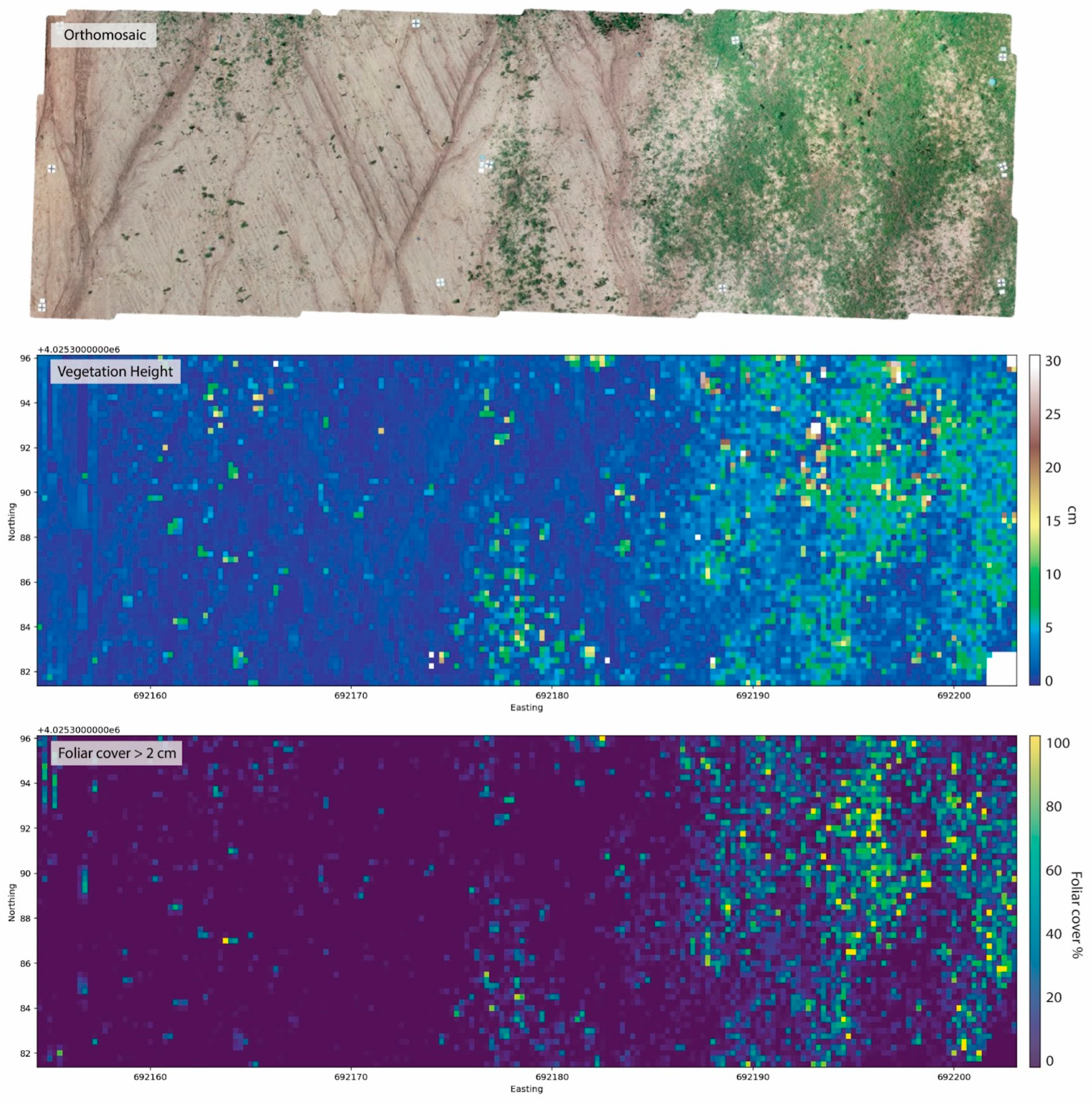
To test the vegetation height and foliar cover algorithms with real-world data for a UAV-based object detection task, we created nine DSMs from eight different test fields that span a diversity of environments, including grass, dirt, tarp, gravel, high grass, flower fields, and salt flats (Section 3.2). Figure 4 shows an example of extracting Hv and Fcover from a DSM of one of eight inert minefield environments in this study.

2.4. Vegetation Height and Cover Verification

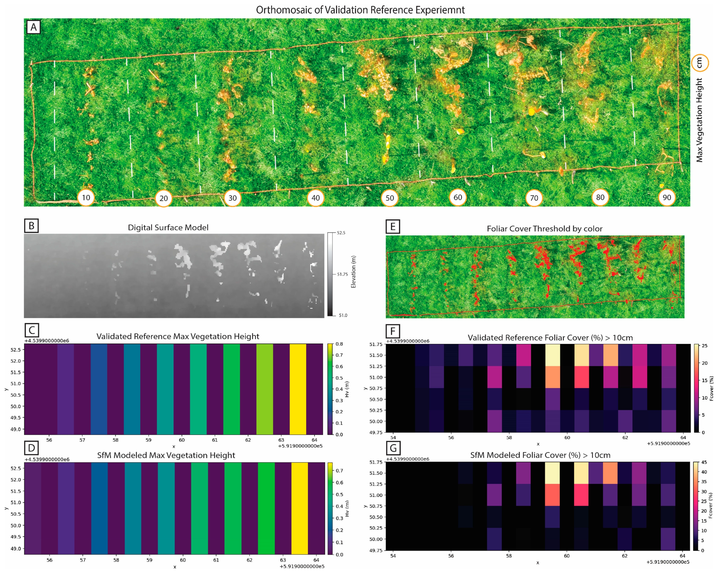
In order to quantify the errors associated with extracting vegetation and cover from UAV imagery, we collected independent ground-truth vegetation height and cover measurements to compare with the SfM algorithmic approaches in Section 2.3. The experiment consisted of a 9 × 2 m area on a grassy pitch with 18 columns spaced 0.5 m apart. Every other column had branches and sticks (vegetation) that were measured to a specific maximum height using a meter stick and stuck into the ground. The vegetation height for the columns ranged from 0 cm to 90 cm in increments of 10 cm. Between each column with “vegetation” was a column without any vegetation to isolate the height and cover measurements in post-processing. In general, the individual columns of a specific vegetation height increased in density of coverage from sparse to dense from south to north. All the branches and sticks were spray-painted bright orange to be visually distinct from the background grass. This allowed for color-based thresholding to estimate percent foliar cover from the RGB imagery. The smallest dimension of this vegetation was on the order of 0.5 cm in width. To estimate the validated reference Fcover, we used an image processing software, ImageJ version 1.53, and applied a color-based thresholding to isolate the orange-painted vegetation from the background [44]. From this mask, we calculated the percent area that was orange for a discrete 0.5 m2 cell. Figure 5 shows the field and the color threshold. Once the field was set up, we collected a grid-style UAV survey in low wind conditions with the DJI Phantom 4 Pro at 10 m flight height above the field with 80% frontal overlap and 80% side-lap. This survey was processed using Pix4DMapper, resulting in an orthomosaic and a DSM with a resolution of 0.27 cm/pix used to extract the Hv and Fcover.
To calculate the maximum vegetation height error, we took the maximum vegetation height per column using the algorithmic approach described in Section 2.3 and calculated the average least squares error compared to the validated reference heights. To calculate the Fcover error, we calculated the least square error per cell between the algorithmic approach in Section 2.3 and the validated reference color threshold.

3. Results

3.1. Effect of Occlusion on Recall

In this section, we investigate the effect of occlusion on recall for the detection of the PFM-1 anti-personnel mine using a trained YOLOv8 convolutional neural network model. After generating 7930 synthetic-grass images (spanning a range of increasing grass density, widths, and lengths for 9 base images) with each image containing a single PFM-1, the images are passed through the trained model. The trained model makes predictions for each image, and we record if the item was detected or not and the confidence score of each prediction. The base images have no other objects in them besides the singular PFM-1, and the results show that there were no false positives detected in any of the images. Due to this result, the precision of the model in this context of limited base images with no false positive objects is 1.0. The detection for each image is binary, so to assess the recall due to occlusion, we sorted all of the images into bins for each percent occlusion (ex. 0–1%, 1–2%, etc.) and calculated the mean detection rate per bin. The occlusion per image is calculated by finding the percent grass occlusion that overlays the PFM-1 segmentation mask.
Figure 6 shows the result of this analysis, where each dot is the mean recall per occlusion percentage. We fit a negative sigmoid curve to model the recall (or “detectability”) as a function of foliar cover, given as follows:
R e c a l l ( F c o v e r ) = 1 1 1 + e   k   ( F c o v e r X 0 )
where k = −0.132379 and X0 = 35.80863 are empirically determined coefficients.
The least squares error for recall between the synthetic data and the fitted sigmoid function is 0.063, with an R2 value of 0.996. Given the nearly perfect fit of the model, the recall for the synthetic grass dataset is entirely dependent on percent occlusion and can be modeled with a high degree of accuracy. Between 20 and 60% occlusion, the change in occlusion is the greatest, with the steepest gradient at 36% occlusion with a δ   R e c a l l δ   o c c l u s i o n = 0.03 (as shown in Supplemental Figure S2).
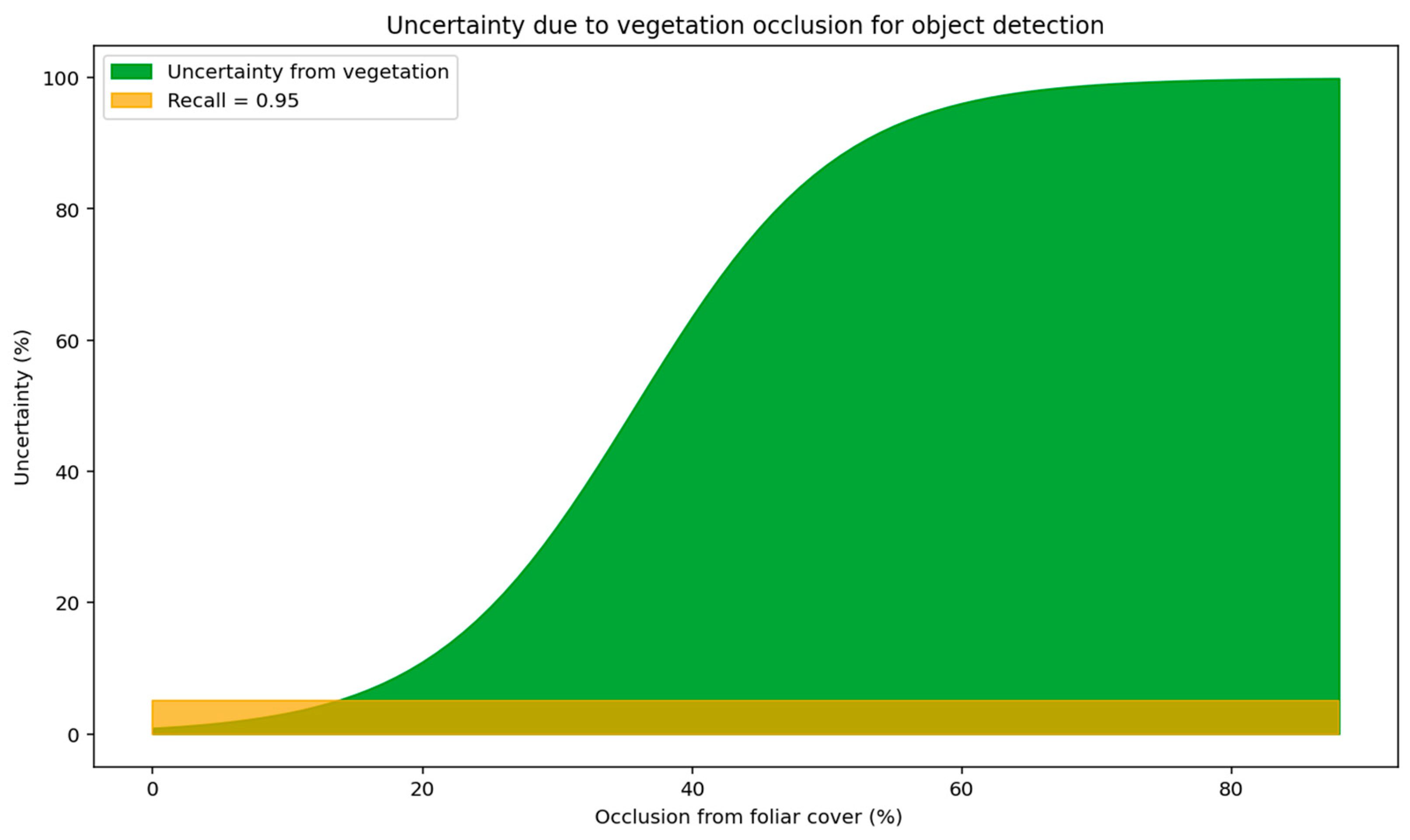
The uncertainty due to vegetation for this model as described in Equation (4) is illustrated in Figure 7. At occlusion rates greater than 15%, uncertainty due to foliar cover quickly becomes the dominant source of uncertainty in our task of detecting an object in a vegetated environment from nadir UAV imagery. This illustrates the importance of quantifying the effect of vegetation occlusion in relevant object detection tasks such as landmine detection.
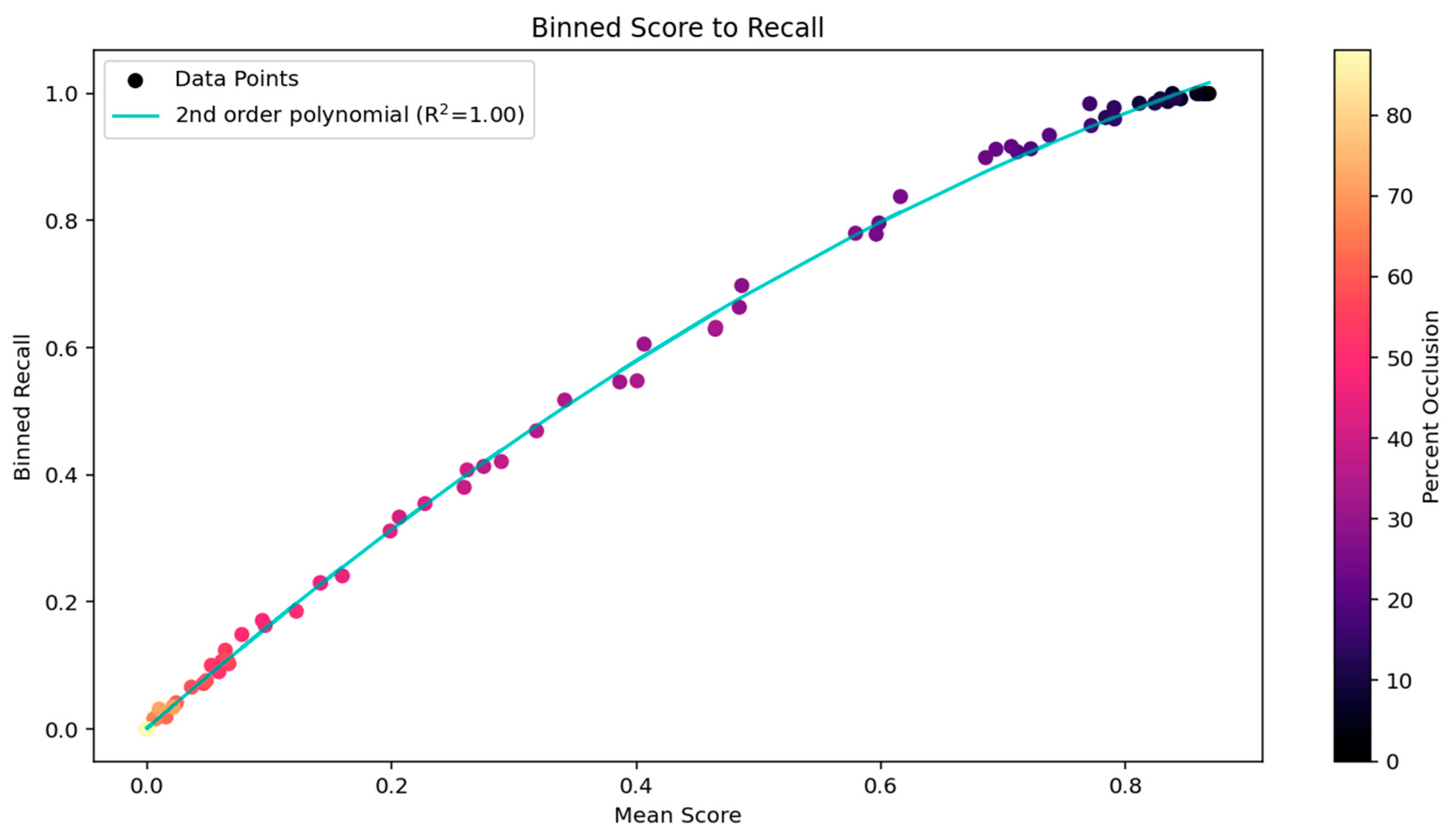
Figure 8 shows that the score and recall (detection rate) are strongly correlated (R2 = 0.999) and are both functions of percent occlusion (foliar cover). This indicates that score can be a proxy for foliar cover in an ideal environment without taking into account other sources of uncertainty, such as camera artifacts and other biases inherent to a specific object detection model. The relationship between score and recall is well fit by a second-order polynomial and is not a simple linear relationship due to the sigmoid nature of the relationship between percent occlusion and recall.

Explained Variance Based on Occlusion Factors

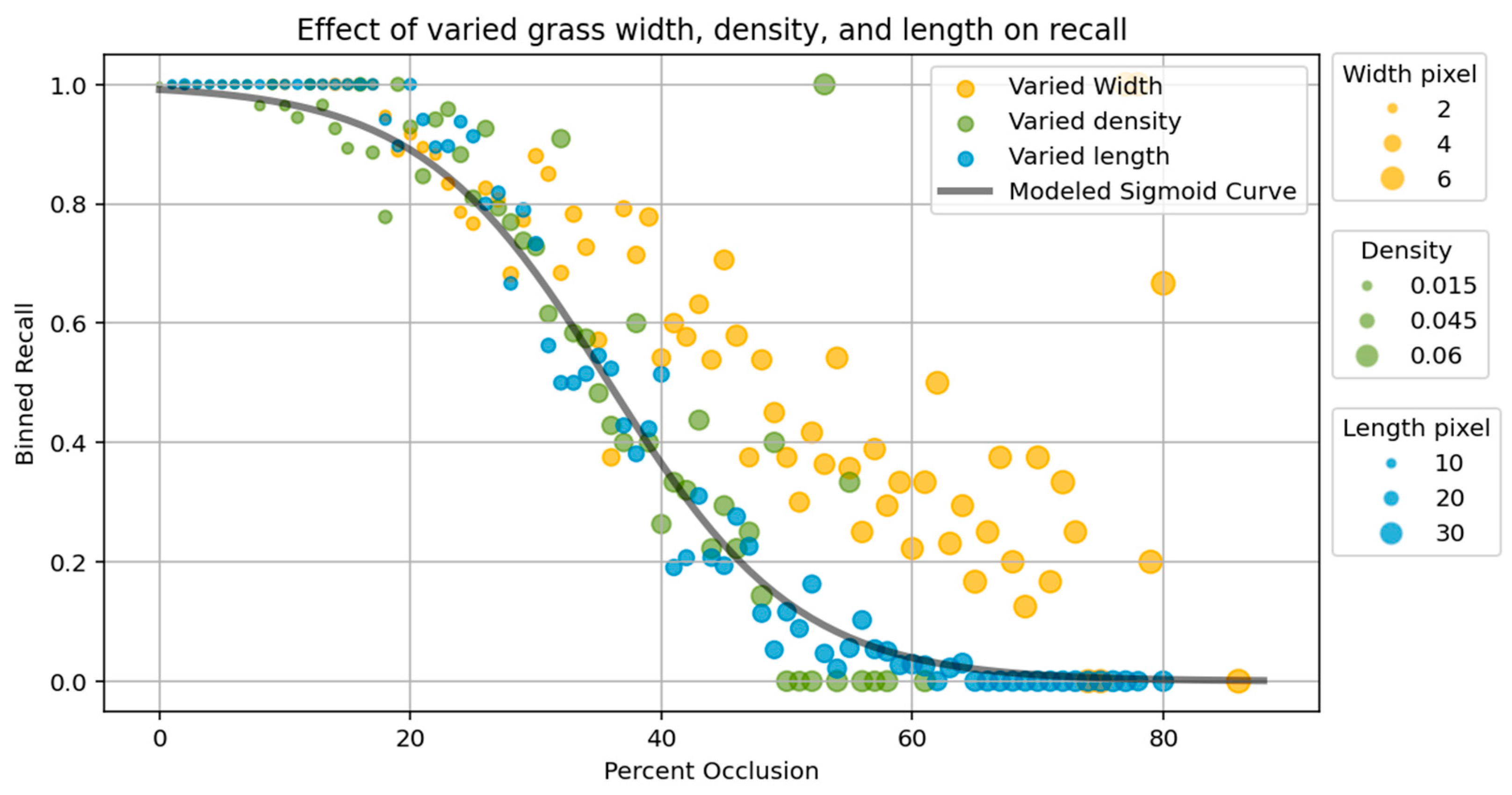
The recall of a UAV-based object detection model is a function of the percent occlusion (foliar cover). In this section, we investigate how varying the density, length, and width of the synthetically generated grass influences the recall. To address this question, we generated three additional synthetic occlusion datasets to isolate each variable. The three parameters that determine the “growth” of the synthetic grass are density (roots per area), length (in pixels), and width (in pixels).
The plot above shows three datasets along with the sigmoid model from all the synthetic grass data in Section 3.1 (Figure 9). The green points have a varied density and a fixed length and width, with the points being sized by increasing density. The blue points have a varied length and a fixed width and density, with the points being sized by increasing length. The orange points have a varied width and a fixed length and density, with the points being sized by increasing width. The varied density and length dataset fit well to the sigmoid curve for all the data, implying density and length have no significant effect on detection rate besides correlating with increasing occlusion percentage. After around 30% occlusion, the varied-width dataset seems to diverge slightly from the main sigmoid function. In other words, for objects with >30% occlusion, the recall for “wide grass” is higher than for the rest of the dataset.

3.2. Empirical Recall with Occlusion

In this section, we compare the modeled-derived detection rates based on foliar cover with actual detection rates from a trained CNN in eight different test mine field environments (Figure 10). The diversity of environments is meant to span a realistic subset of where EO and mines are found. One shortcoming is that the dataset does not adequately cover the high and dense vegetation endmembers and is more heavily skewed towards sparse, low vegetation environments. Table 1 shows the average Hv, the Fcover greater than 4 cm, the number of UXO detected, and the total number of UXO present.
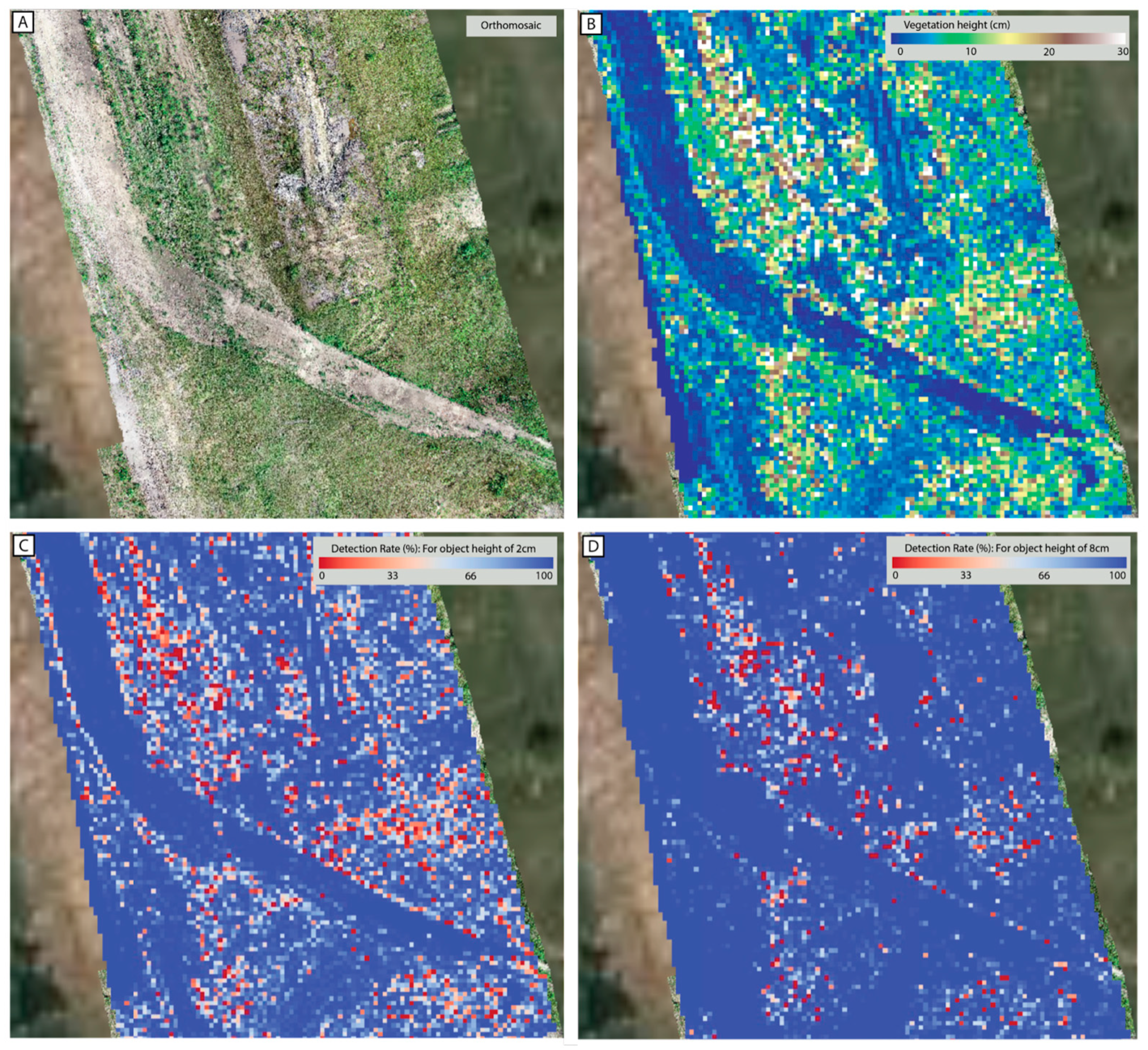
We implement our method to quantify vegetation height and foliar cover to understand how these measurements correlate with occlusion and detection rate in the real world. Figure 11 shows an orthomosaic of a UAV survey and the resultant vegetation height and detectability maps generated from the DSM of a mined area. The bottom panel of the figure illustrates that the “detectability” of an object is dependent on the height of the object. The most apparent feature is the dirt road that diagonally cuts through the map. We can see the vegetation height map, and the detectability maps are able to effectively model this and set the dirt road to have a near-zero vegetation height and a 100% detection rate (or 0% uncertainty due to vegetation). The bottom left panel shows the detectability map for Ho = 2 cm, and the bottom right panel shows the detectability map for Ho = 8 cm. We choose Ho = 2 cm as the lower bound because that is the height of the smallest anti-personnel (AP) mines, with most AP mines between 2 and 8 cm in height. As the object height increases, vegetation that is shorter than the new object height no longer contributes to foliar cover and results in higher detectability for these taller objects. Supplemental Figure S4 demonstrates this further with detectability rate maps for Ho = [2, 4, 6, 8] cm.
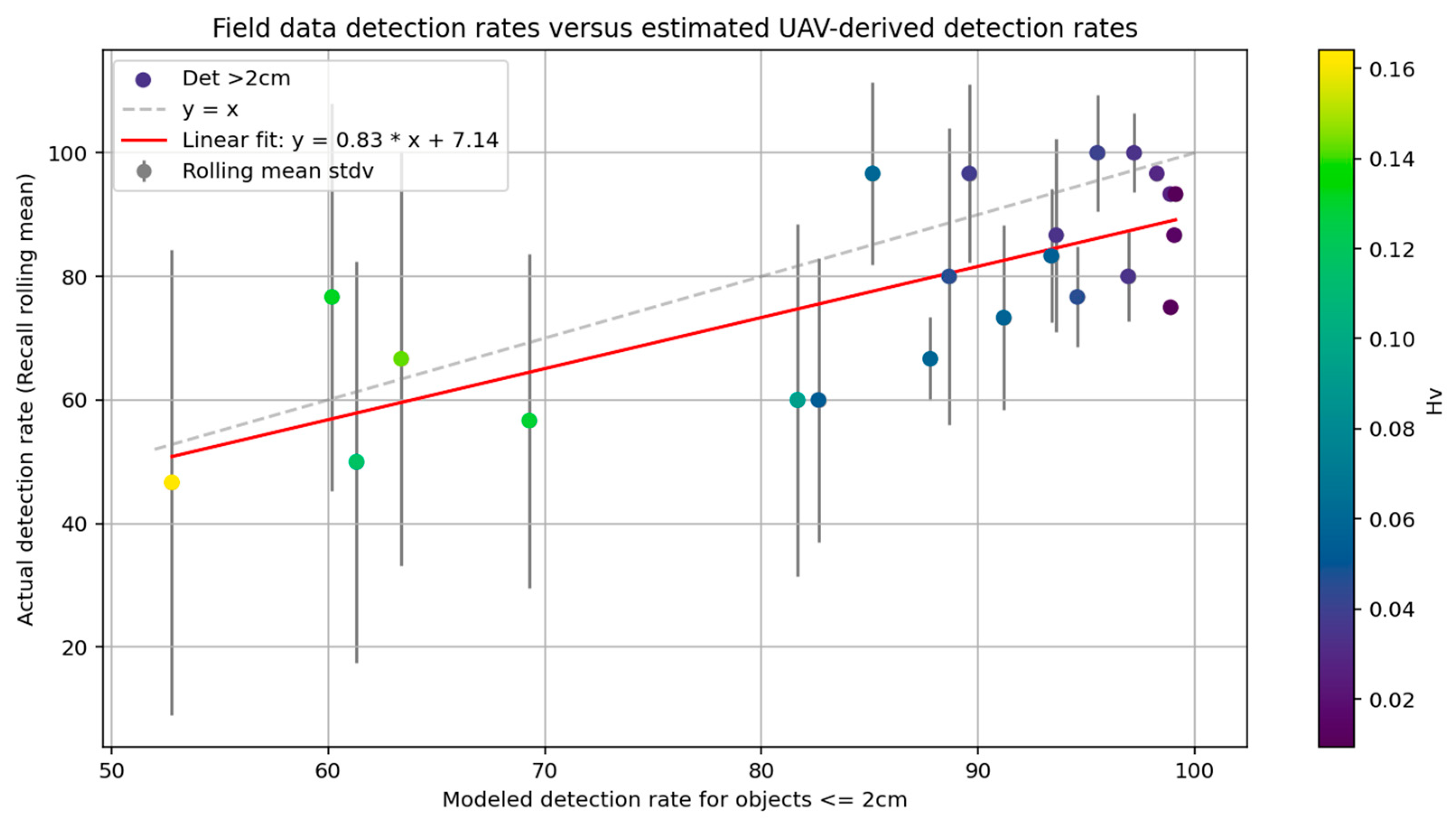
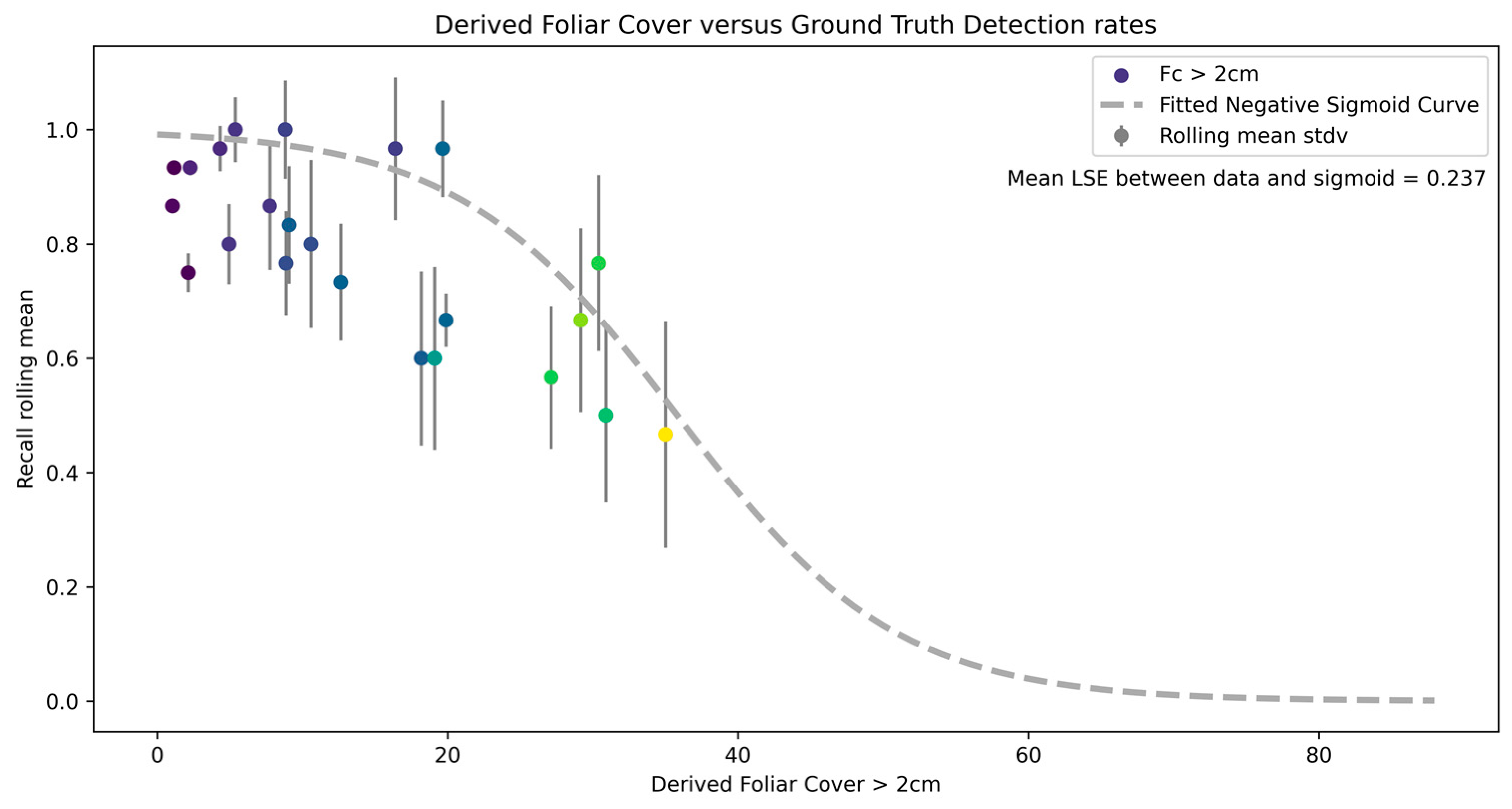
Applying these algorithms and models to the nine DSMs from the test minefields, we are able to compare the relationship between the recall of the machine learning model and the detection rate predicted by the vegetation uncertainty model. Figure 12 shows the rolling-mean recall of the real-world UAV minefield data to the uncertainty model detection rate, following a linear fit of y = 0.83x + 7.14. We used a rolling mean of 30 objects with the most similar estimated foliar cover percentage to allow us to resolve detection rates to a resolution of 0.033 recall due to limitations in the quantity of data available. The standard deviation for the rolling mean recall of each point decreases with an increasing detection rate. This means that objects with low uncertainty due to vegetation have less variance than those with high uncertainty. This is likely because the uncertainty of the vegetation height and vegetation cover model increases with increasing vegetation height. Figure 13 shows the recall rolling mean from the mine fields plotted along the derived sigmoid recall occlusion curve. Most of the data points follow the trend of decreasing recall with increased occlusion but, in general, have detection rates lower than the synthetic data. The mean LSE between the empirical data points and the sigmoid curve is 0.24. This discrepancy will be discussed in Section 4.1.2.

3.3. Vegetation Height and Cover Error

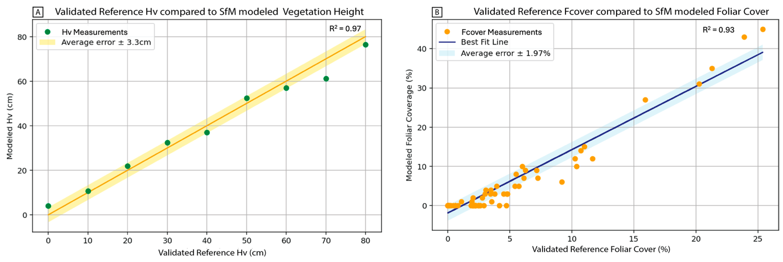
The validated reference vegetation height compared to the modeled vegetation height yielded an average absolute error of ±3.3 cm with an R2 = 0.97. In general, the results show this algorithm is very well constrained for estimating vegetation height within ±3.3 cm. The highest misfit for vegetation height occurred at 70 cm on the validated reference (x-axis), and the best fit height was at 10 cm. We also found that the average error for the modeled foliar cover compared to the validated reference color threshold was well captured through a linear regression, which yielded ±1.97% cover and an R2 = 0.93.

4. Discussion

4.1. Interpretation of Results

4.1.1. Effect of Occlusion on Recall

We speculate that recall as a function of percent occlusion (Figure 6) fits a sigmoid curve due to the combination of robustness to noise, a non-linear relationship between occlusion and recall, and critical thresholds. Since recall for a fully unoccluded object approaches 100% and the CNN is robust to some degree of noise, the initial drop in recall is insignificant for very low occlusion instances. Because we are looking at binned recall, as occlusion increases, the chances of more and more salient features being occluded increase, causing a drop in recall. This trend continues until it approaches a critical threshold at which all salient features are occluded, resulting in the recall approaching zero. Operationally, this means that the object detection model is barely affected by occlusion less than 20%, greatly affected from 20 to 60% occlusion, and then is effectively undetectable at the tail end of the sigmoid curve past 60% occlusion.
For the synthetic grass width varied dataset (orange dots) in Figure 9, we speculate that the divergence from the modeled sigmoid curve is because the wide grass occludes larger singular patches of the object, leaving some salient features visible. It is possible that this is a model-specific effect. While the denser, thinner grass covers thin linear patches of pixels over the entire object (partially occluding many salient features), making it harder to identify for the object detection model. This is akin to an eye patch (wide, less dense) versus long hair (thinner, more dense) over someone’s eye. Anomalies such as the varied width of data points at 1.0 recall are the result of insufficient data for the recall bin.

4.1.2. Empirical Recall with Occlusion

While the data in Figure 13 show a general trend that follows the synthetic-occlusion-derived sigmoid curve, on average, it has lower detection rates than predicted. We anticipate that the field results have a lower detection rate due to a combination of real-world factors, including camera artifacts such as motion blur and lighting saturation, artifacts from SfM photogrammetry, variable resolutions from differing flight heights and cameras, and other sources of occlusion like dust, dirt, or snow (over an item or camera lens) that are not captured in this model, among other factors. In the synthetic grass dataset, the only variable that was changed was the occlusion. There were no camera artifacts such as motion blur, no artifacts from photogrammetry, and lower resolution due to variable flight heights. The effects of these other factors on detection rate are not quantified and likely non-linear (or do not follow the synthetic occlusion sigmoid curve), and thus can cause deviations from the synthetic derived function shown in the dashed gray line.

4.1.3. Vegetation Height and Cover Error

In Figure 14, the linear regression has a slope greater than 1, meaning that the modeled vegetation cover overestimated the true foliar cover, but that overestimation scaled with increasing foliar cover. This overestimation compared to the validated reference data seems to result from the small, uncovered areas between the leaves that are modeled as larger blob-like surfaces without small gaps or holes in the DSM. The blob-like artifacts may be due to factors that reduce the matched keypoint density, such as vegetation moving in the wind, small parallax distances from nadir imagery, or the limited resolution of the DSM to resolve small gaps. These factors create artifacts that are difficult for an object detection model to see through and result in the small gaps becoming effectively occluded areas above the object. In the end, even though the vegetation coverage is overestimated by (Fcover Modeled ≈ 1.5 × Fcover Ground-truth), due to the SfM artifacts in the orthomosaic and DSM, the effective occlusion is very well modeled by the vegetation coverage model.

4.2. Limitations

While our model verification yielded relatively small error bars, there are still limitations inherent to the methodology. The first is that the recall versus percent occlusion function is model- and object-specific. While the sigmoid function (Equation (5)) may be a suitable first approximation for the detectability of other object types with increasing amounts of foliar cover, it is not fully generalizable because different objects will have different salient features built into the latent space of the object detection model. To address this limitation, it is best for someone to generate either real or synthetic data on various occlusions of the object of interest and fit a sigmoid function to the model results. Additionally, the effect of varying occlusion is heavily dependent on the latent representation of the object in the model and can vary widely depending on the data that the model was trained on. Two models with identical architectures can have different representations of the same object when trained on different datasets.
As seen in Figure 13, the real-world sigmoid curve deviated from the sigmoid curve generated with purely synthetic data. This illustrates that there are multiple variables in real-world UAV imagery that can decrease the recall, and to achieve a completely unbiased comparison of the synthetic recall to the empirical recall would require quantifying other sources of uncertainty such as motion blur and camera artifacts. Despite this limitation, we see that the data roughly follows the synthetic recall-occlusion curve from 0–35% occlusion, indicating that vegetation is the dominant source of uncertainty for this object detection task.
Furthermore, there are limitations for deriving the vegetation height and foliar cover from the structure-from-motion photogrammetry survey. First, the resolution of the DSM (dependent on the flight height and camera of the UAV) will dictate the thickness and size of the vegetation you can resolve. The UAV landmine dataset in this study was captured at 10 m height with an average ground sampling distance of 0.25 cm/pix. This allowed us to resolve subcentimeter-scale vegetation profiles matching closely with the validated reference datasets (Figure 14). In the case where the DSM has a much lower resolution (on the scale of 10 s of centimeters or meters), deriving Hv and Fcover will be subject to much higher uncertainty or will be unresolvable. Using a high-pass filter preserves all the high-frequency artifacts and is subject to noise or erroneous pixel values. To mitigate the effect of noise, we set the max Hv to be the vegetation height of the 99th percentile, removing any anomalously high pixels from the DSM [41,42,43]. The accuracy of the vegetation height estimates will depend on the type and density of vegetation present. In dense vegetation and forests, this method might not work well due to the overlapping canopies where there is no range in elevation values in a 0.5 m2 cell due to the inability of optical remote sensing to penetrate vegetation. A potential way to handle this situation would be to discretize the raster into larger (>0.5 m2) cells in hopes of modeling a ground pixel through the foliage, at the expense of spatial resolution. Furthermore, because the measurement error in Hv propagates and influences the accuracy of Fcover measurement, utilizing the relative difference between the object height and Hv could help better quantify the uncertainty in calculating Fcover. Heavy shadows or poor lighting (or white balance/saturation issues) in the imagery can compromise the quality and accuracy of the DSM due to difficulty in extracting matching key points potentially leading to gaps or artifacts. Wind can also degrade DSM accuracy by moving vegetation, making keypoint matching difficult.

4.3. Vegetation Height Model Approaches

The basic principle for generating a vegetation height model involves subtracting a DSM from a DTM [45]. This process removes the underlying topography, and what remains is a vegetation height or canopy height model. DiGiacomo et al., 2020, describe three methods commonly used to derive a DTM to model salt marsh vegetation height. These include manually selecting or using NDVI to identify ground points, which are then interpolated to create a DTM, or interpolating LiDAR-derived ground points [46]. In crop monitoring, another method to estimate crop height is to collect a SfM survey in the off-season before crops have grown and use this to construct a DTM for the field [47]. This method works well but requires two flights at different times of year as well as ground-control points to georeference the two datasets [42]. These methodologies can be used to create detectability maps (Equation (5)) and integrate with the proposed workflow, but they have logistical and technical drawbacks compared to single flight RGB SfM imagery that is inherently part of UAV object detection tasks.

4.4. Improving Robustness of Object Detection from Vegetation Occlusion

While quantifying the uncertainty due to vegetation occlusion is important, a natural next question is how one can improve a deep learning model to achieve more robust detection rates in the face of occlusion. One approach to overcoming this challenge is to build a training dataset with various levels of occlusion in its natural environment or introduce synthetic occlusion in the training set [26]. Another approach designed to mitigate the effect of occlusion is to use a data augmentation technique called random erasing. Random erasing functions by randomly removing (erasing) parts of the object and is designed to make a model more robust to occlusion by preventing it from overfitting to specific features of the object [48,49]. Lastly, modifying or changing the model architecture itself may yield improvements in the face of occlusion, such as employing instance segmentation or semantic segmentation [50,51]. Several alternative deep learning architectures have been proposed to address the issue of occlusion, but a characterization of the effect that occlusion has on existing models has been under research. Segmentation is used to preserve the occluded features in the latent representation of the object. In a study conducted by a team at Stanford, a hybrid detection segmentation approach yielded a 2% gain in precision when compared with a traditional detection model on the pascal VOC2007 dataset [52]. This shows promise in the creation of new architectures that may be more robust against occlusion for the detection task, but it does not advance our ability to assess the effect of occlusion. Alternatively, spectral-based approaches, such as hyperspectral, multispectral, and thermal infrared imaging (with or without deep learning), show promise for the detection of man-made objects in vegetated environments. Objects such as landmines can be detected based on their distinct spectral signatures that differ from the surrounding environment [20,53,54,55,56]. These methods are still affected by vegetation occlusion, and therefore quantifying the uncertainty due to vegetation occlusion is an important avenue for future studies for the implementation of such methodologies. Overall, a combination of data-driven techniques, custom model architectures, and additional data streams, such as multispectral imaging, may yield improvements for object detection in occluded scenes.

4.5. Application to Humanitarian Mine Action

This paper implements a model that considers the effect of vegetation on UAV-based object detection for landmines and UXO. This model has direct implications in humanitarian mine action for (1) putting mine detection predictions into environmental context, (2) determining the optimal regions to conduct UAV surveys for landmine detection, and (3) finding the best times for conducting these types of surveys. This model helps put predictions into context in that if one mine is found in a region with a 10% detectability, there are likely nine other mines in that area that were not found. Conversely, if no items are detected in a region with 100% detectability (0% uncertainty due to vegetation), then there is a high level of confidence that there is no surface contamination in that area, which can be a lower priority for mine clearance resource allocation. Broadly, this model can also be used to increase the situational awareness of demining personnel, as it can highlight dangerous and less dangerous areas when paired with an object detection model such as that presented by Baur and Steinberg et al. in 2020 [18]. For points (2) and (3), prior to the application of an object detection model, this detectability due to vegetation has wide implications for determining the best locations and times of year to conduct UAV-based detection surveys. If the rate of vegetation growth is known, it is possible to apply that rate to the current vegetation height map to extrapolate detection rates into the future, essentially providing a time series of UAV-based detection rates for a given environment. Future studies could investigate detectability versus crop growth cycles and land use in Ukraine [57] for wide-area assessment and prioritization of UAV-based detection surveys.

4.6. Broader Applications and Implications

In this paper, we lay the framework for developing a custom uncertainty model for quantifying the effect of vegetation on the performance of an object detection model. Figure 15 shows the workflow diagram for this study and how all the components fit together.
We then take this one step further and develop two algorithms to derive vegetation height and coverage from UAV imagery, allowing us to map the uncertainty due to vegetation over an orthomosaic collected during a UAV survey. This workflow is especially relevant for small object detection tasks where quantifying how occlusion affects detection rates is a concern. This workflow and model can be applied to a wide variety of object detection applications in the real world. The vegetation height and foliar coverage models on their own can be useful as an inexpensive, first-order approximation of biomass, a tool for crop monitoring, and a way to plan accessible routes for search and rescue operations.

5. Conclusions

In this study, we took a unique approach combining real-world remote sensing data, image processing, deep learning and computer vision, and synthetic data generation to investigate how foliar cover affects the detection rate for UAV-based object detection.
This study’s main contributions can be summarized as follows:
  • Novel algorithm to extract vegetation height and foliar cover from a UAV-derived Digital Surface Model.
  • Generating synthetic grass growth over an object to quantify the effect of occlusion with increasing foliar cover on detection rates of small objects in the natural environment.
  • Developing an occlusion-based vegetation uncertainty model that combines (1) and (2) to create a “detectability” map over an orthomosaic for a deep learning object detection model.
  • Applying the uncertainty model in (3) to a real-world test case for UAV-based landmine detection.
Using the PFM-1 anti-personnel landmine as a case study, we found the recall of the trained neural network is modeled as a sigmoid curve, where essentially 0–20% foliar cover had very little effect on detection rates. From 20–60% foliar cover, there was a steep decrease in recall from around 0.90 at 20% cover to less than 0.10 at 60% cover, and from 60–100% foliar cover, the recall (detection rate) was near 0. We then apply this sigmoid function relating foliar cover to detection rates to a structure-from-motion-derived vegetation height and cover model, allowing us to create uncertainty maps (or detection rate maps) for UAV-based object detection tasks. This approach is cost-effective and easy to implement within the existing UAV-based object detection frameworks, providing crucial context for detection rates in vegetated environments. Due to these reasons, this model and approach can have widespread implications for determining the optimal regions and times of year to conduct UAV flights for object detection. Overall, modeling detection rate as a function of vegetation cover for deep learning object detection models in natural environments is crucial for putting predictions into context and quantifies one of the most challenging aspects of UAV-based object detection.

Supplementary Materials

The following supporting information can be downloaded at: https://www.mdpi.com/article/10.3390/rs16122046/s1, Text S1. Discussion on LiDAR versus SfM photogrammetry. Text S2. Discussion on shadow as a source of occlusion. Figure S1. Number of data in each percent occlusion bin for the synthetic dataset. Figure S2. This plot shows the rate of change in recall with increased occlusion as the first derivative of the sigmoid function. The maximum change in recall is at 36% occlusion, as indicated by the orange dot. Figure S3. This plot illustrates the residuals between the observed data points and the fitted negative sigmoid curve. The residuals are calculated as the difference between the observed values of the recall rolling mean and the values predicted by the fitted curve. A red-dash horizontal line at zero indicates the point where the predicted values perfectly match the observed values. Residuals above the line indicate that the observed values are higher than predicted, while residuals below the line indicate that the observed values are lower than predicted. Figure S4. This figure illustrates that the “detectability” of an object is dependent on the height of the object. The top left panel shows Ho = 2 cm, with a clear reduction in detectability on the vegetated (right) side of the field. As the object height increases, vegetation that is shorter than the new object height no longer contributes to foliar cover and results in higher detectability for these taller objects. Figure S5. This plot shows the absolute error (percentage) of modeled foliar cover as a function of foliar cover. Notice how the error increases with increasing foliar cover. References [41,45,58,59,60,61,62,63,64,65,66] are cited in Supplementary Materials.

Author Contributions

Conceptualization, J.B., G.S. and K.D.; methodology, J.B. and K.D.; validation, J.B.; formal analysis, J.B.; investigation, J.B.; data curation, J.B., G.S. and K.D.; writing—original draft preparation, J.B. and K.D.; writing—review and editing, J.B., G.S., K.D. and F.O.N.; visualization, J.B.; supervision, F.O.N. All authors have read and agreed to the published version of the manuscript.

Funding

This research received no external funding.

Data Availability Statement

The data presented in this study are available on request from the corresponding author. The data are not publicly available due to the sensitive nature of the application of landmine detection in minefields in conflict and post conflict nations.

Acknowledgments

The authors would like to thank John Frucci and Billy Magalassi from the OSU Global Consortium for Explosive Hazard Mitigation for access to the explosives range and inert ordnance, and Taylor Mitchell from the OSU Unmanned Systems Research Institute for assistance with data collection. We would also like to thank Alex Nikulin and Tim de Smet from Binghamton University and Aletair LLC for access to UAVs during the summer 2022 data collection season. Lastly, we would like to thank Tess Jacobson, Sam Bartusek, Claire Jasper, Conor Bacon, and Daniel Babin for helping set up the orange stick experiment in the Lamont soccer fields.

Conflicts of Interest

The authors declare no conflicts of interest.

References

  1. Deng, J.; Dong, W.; Socher, R.; Li, L.J.; Li, K.; Fei-Fei, L. Imagenet: A large-scale hierarchical image database. In Proceedings of the 2009 IEEE Conference on Computer Vision and Pattern Recognition, Miami, FL, USA, 20–25 June 2009; IEEE: New York, NY, USA, 2009; pp. 248–255. [Google Scholar]
  2. Krizhevsky, A.; Sutskever, I.; Hinton, G.E. Imagenet classification with deep convolutional neural networks. In Proceedings of the Advances in Neural Information Processing Systems, Lake Tahoe, NV, USA, 3–6 December 2012; Volume 25. [Google Scholar]
  3. Redmon, J.; Divvala, S.; Girshick, R.; Farhadi, A. You only look once: Unified, real-time object detection. In Proceedings of the IEEE Conference on Computer Vision and Pattern Recognition, Las Vegas, NV, USA, 26 June–1 July 2016; pp. 779–788. [Google Scholar]
  4. Girshick, R. Fast r-cnn. In Proceedings of the IEEE International Conference on Computer Vision, Santiago, Chile, 7–13 December 2015; pp. 1440–1448. [Google Scholar]
  5. Ren, S.; He, K.; Girshick, R.; Sun, J. Faster r-cnn: Towards real-time object detection with region proposal networks. In Proceedings of the Advances in Neural Information Processing Systems 28 (NIPS 2015), Montreal, QC, Canada, 7–12 December 2015; Volume 28. [Google Scholar]
  6. Liu, W.; Anguelov, D.; Erhan, D.; Szegedy, C.; Reed, S.; Fu, C.Y.; Berg, A.C. Ssd: Single shot multibox detector. In Proceedings of the Computer Vision–ECCV 2016: 14th European Conference, Amsterdam, The Netherlands, 11–14 October 2016; Proceedings, Part I 14. Springer International Publishing: Berlin/Heidelberg, Germany, 2016; pp. 21–37. [Google Scholar]
  7. Daponte, P.; De Vito, L.; Glielmo, L.; Iannelli, L.; Liuzza, D.; Picariello, F.; Silano, G. A review on the use of drones for precision agriculture. In IOP Conference Series: Earth and Environmental Science; IOP Publishing: Bristol, UK, 2019; Volume 275, p. 012022. [Google Scholar]
  8. James, M.R.; Carr, B.; D’Arcy, F.; Diefenbach, A.; Dietterich, H.; Fornaciai, A.; Lev, E.; Liu, E.; Pieri, D.; Rodgers, M.; et al. Volcanological applications of unoccupied aircraft systems (UAS): Developments, strategies, and future challenges. Volcanica 2020, 3, 67–114. [Google Scholar] [CrossRef]
  9. Nex, F.; Remondino, F. UAV for 3D mapping applications: A review. Appl. Geomat. 2014, 6, 1–15. [Google Scholar] [CrossRef]
  10. Amoukteh, A.; Janda, J.; Vincent, J. Drones Go to Work. BCG Global. 2017. Available online: https://www.bcg.com/publications/2017/engineered-products-infrastructure-machinery-components-drones-go-work (accessed on 10 January 2024).
  11. Westoby, M.J.; Brasington, J.; Glasser, N.F.; Hambrey, M.J.; Reynolds, J.M. ‘Structure-from-Motion’photogrammetry: A low-cost, effective tool for geoscience applications. Geomorphology 2012, 179, 300–314. [Google Scholar] [CrossRef]
  12. Du, D.; Qi, Y.; Yu, H.; Yang, Y.; Duan, K.; Li, G.; Zhang, W.; Huang, Q.; Tian, Q. The unmanned aerial vehicle benchmark: Object detection and tracking. In Proceedings of the European Conference on Computer Vision (ECCV), Munich, Germany, 8–14 September 2018; pp. 370–386. [Google Scholar]
  13. Mittal, P.; Singh, R.; Sharma, A. Deep learning-based object detection in low-altitude UAV datasets: A survey. Image Vis. Comput. 2020, 104, 104046. [Google Scholar] [CrossRef]
  14. Cao, Y.; He, Z.; Wang, L.; Wang, W.; Yuan, Y.; Zhang, D.; Zhang, J.; Zhu, P.; Van Gool, L.; Han, J.; et al. VisDrone-DET2021: The vision meets drone object detection challenge results. In Proceedings of the IEEE/CVF International Conference on Computer Vision, Montreal, BC, Canada, 11–17 October 2021; pp. 2847–2854. [Google Scholar]
  15. Pham, M.T.; Courtrai, L.; Friguet, C.; Lefèvre, S.; Baussard, A. YOLO-Fine: One-stage detector of small objects under various backgrounds in remote sensing images. Remote Sens. 2020, 12, 2501. [Google Scholar] [CrossRef]
  16. Hamylton, S.M.; Morris, R.H.; Carvalho, R.C.; Roder, N.; Barlow, P.; Mills, K.; Wang, L. Evaluating techniques for mapping island vegetation from unmanned aerial vehicle (UAV) images: Pixel classification, visual interpretation and machine learning approaches. Int. J. Appl. Earth Obs. Geoinf. 2020, 89, 102085. [Google Scholar] [CrossRef]
  17. Zangerl, U.; Haselberger, S.; Kraushaar, S. Classifying Sparse Vegetation in a Proglacial Valley Using UAV Imagery and Random Forest Algorithm. Remote Sens. 2022, 14, 4919. [Google Scholar] [CrossRef]
  18. Baur, J.; Steinberg, G.; Nikulin, A.; Chiu, K.; de Smet, T.S. Applying deep learning to automate UAV-based detection of scatterable landmines. Remote Sens. 2020, 12, 859. [Google Scholar] [CrossRef]
  19. Barnawi, A.; Budhiraja, I.; Kumar, K.; Kumar, N.; Alzahrani, B.; Almansour, A.; Noor, A. A comprehensive review on landmine detection using deep learning techniques in 5G environment: Open issues and challenges. Neural Comput. Appl. 2022, 34, 21657–21676. [Google Scholar] [CrossRef]
  20. Bajić, M., Jr.; Potočnik, B. UAV Thermal Imaging for Unexploded Ordnance Detection by Using Deep Learning. Remote Sens. 2023, 15, 967. [Google Scholar] [CrossRef]
  21. Harvey, A.; LeBrun, E. Computer Vision Detection of Explosive Ordnance: A High-Performance 9N235/9N210 Cluster Submunition Detector. J. Conv. Weapons Destr. 2023, 27, 9. [Google Scholar]
  22. Baur, J.; Steinberg, G.; Nikulin, A.; Chiu, K.; de Smet, T. How to implement drones and machine learning to reduce time, costs, and dangers associated with landmine detection. J. Conv. Weapons Destr. 2021, 25, 29. [Google Scholar]
  23. Coulloudon, B.; Eshelman, K.; Gianola, J.; Habich, N.; Hughes, L.; Johnson, C.; Pellant, M.; Podborny, P.; Rasmussen, A.; Robles, B.; et al. Sampling vegetation attributes. In BLM Technical Reference; Bureau of Land Management, National Business Center: Denver, CO, USA, 1999; Volume 1734. [Google Scholar]
  24. Dong, Z.; Lv, P.; Zhang, Z.; Qian, G.; Luo, W. Aeolian transport in the field: A comparison of the effects of different surface treatments. J. Geophys. Res. Atmos. 2012, 117. [Google Scholar] [CrossRef]
  25. Bokhorst, S.; Pedersen, S.H.; Brucker, L.; Anisimov, O.; Bjerke, J.W.; Brown, R.D.; Ehrich, D.; Essery, R.L.H.; Heilig, A.; Ingvander, S.; et al. Changing Arctic snow cover: A review of recent developments and assessment of future needs for observations, modelling, and impacts. Ambio 2016, 45, 516–537. [Google Scholar] [CrossRef] [PubMed]
  26. Saleh, K.; Szénási, S.; Vámossy, Z. Occlusion handling in generic object detection: A review. In Proceedings of the 2021 IEEE 19th World Symposium on Applied Machine Intelligence and Informatics (SAMI), Herl’any, Slovakia, 21–23 January 2021; IEEE: New York, NY, USA, 2021; pp. 000477–000484. [Google Scholar]
  27. Dalborgo, V.; Murari, T.B.; Madureira, V.S.; Moraes, J.G.L.; Bezerra, V.M.O.; Santos, F.Q.; Silva, A.; Monteiro, R.L. Traffic Sign Recognition with Deep Learning: Vegetation Occlusion Detection in Brazilian Environments. Sensors 2023, 23, 5919. [Google Scholar] [CrossRef] [PubMed]
  28. ICBL-CMC. International Campaign to Ban Landmines, Landmine Monitor 2023; ICBL-CMC: Geneva, Switzerland, 2023. [Google Scholar]
  29. GICHD. Difficult Terrain in Mine Action; International Center for Humanitarian Demining: Geneva, Switzerland, 2023. [Google Scholar]
  30. Tuohy, M.; Greenspan, E.; Fasullo, S.; Baur, J.; Steinberg, G.; Zheng, L.; Nikulin, A.; Clayton, G.M.; de Smet, T. Inspiring the Next Generation of Humanitarian Mine Action Researchers. J. Conv. Weapons Destr. 2023, 27, 7. [Google Scholar]
  31. National Mine Action Authority; GICHD. Explosive Ordnance Risk Education Interactive Map. ArcGIS Web Application. 2023. Available online: https://ua.imsma.org/portal/apps/webappviewer/index.html?id=92c5f2e0fa794acf95fefb20eebdecae (accessed on 10 January 2024).
  32. ICBL-CMC. Cluster Munition Coalition. Cluster Munition Monitor 2023. 2023. Available online: www.the-monitor.org (accessed on 5 December 2023).
  33. Jean-Pierre, K.; Sullivan, J. Press Briefing by Press Secretary Karine Jean-Pierre and National Security Advisor Jake Sullivan; White House: Washington, DC, USA, 2023. [Google Scholar]
  34. Mishra, N.B.; Crews, K.A. Mapping vegetation morphology types in a dry savanna ecosystem: Integrating hierarchical object-based image analysis with Random Forest. Int. J. Remote Sens. 2014, 35, 1175–1198. [Google Scholar] [CrossRef]
  35. Resop, J.P.; Lehmann, L.; Hession, W.C. Quantifying the spatial variability of annual and seasonal changes in riverscape vegetation using drone laser scanning. Drones 2021, 5, 91. [Google Scholar] [CrossRef]
  36. Cayssials, V.; Rodríguez, C. Functional traits of grasses growing in open and shaded habitats. Evol. Ecol. 2013, 27, 393–407. [Google Scholar] [CrossRef]
  37. Jocher, G.; Chaurasia, A.; Qiu, J. Ultralytics YOLOv8, Version 8.0.0 Software; GitHub: San Francisco, CA, USA, 2023. Available online: https://github.com/ultralytics/ultralytics(accessed on 10 January 2024).
  38. Cook, K.L. An evaluation of the effectiveness of low-cost UAVs and structure from motion for geomorphic change detection. Geomorphology 2017, 278, 195–208. [Google Scholar] [CrossRef]
  39. Iglhaut, J.; Cabo, C.; Puliti, S.; Piermattei, L.; O’Connor, J.; Rosette, J. Structure from motion photogrammetry in forestry: A review. Curr. For. Rep. 2019, 5, 155–168. [Google Scholar] [CrossRef]
  40. Pix4D. How to Verify That There Is Enough Overlap between the Images—Pix4D Mapper; Pix4D Support: Denver, CO, USA, 2020. [Google Scholar]
  41. Madec, S.; Baret, F.; De Solan, B.; Thomas, S.; Dutartre, D.; Jezequel, S.; Hemmerlé, M.; Colombeau, G.; Comar, A. High-throughput phenotyping of plant height: Comparing unmanned aerial vehicles and ground LiDAR estimates. Front. Plant Sci. 2017, 8, 2002. [Google Scholar] [CrossRef]
  42. Fujiwara, R.; Kikawada, T.; Sato, H.; Akiyama, Y. Comparison of Remote Sensing Methods for Plant Heights in Agricultural Fields Using Unmanned Aerial Vehicle-Based Structure from Motion. Front. Plant Sci. 2022, 13, 886804. [Google Scholar] [CrossRef]
  43. Malambo, L.; Popescu, S.C.; Murray, S.C.; Putman, E.; Pugh, N.A.; Horne, D.W.; Richardson, G.; Sheridan, R.; Rooney, W.L.; Avant, R.; et al. Multitemporal field-based plant height estimation using 3D point clouds generated from small unmanned aerial systems high-resolution imagery. Int. J. Appl. Earth Obs. Geoinf. 2018, 64, 31–42. [Google Scholar] [CrossRef]
  44. Schneider, C.A.; Rasband, W.S.; Eliceiri, K.W. NIH Image to ImageJ: 25 years of image analysis. Nat. Methods 2012, 9, 671–675. [Google Scholar] [CrossRef]
  45. Lisein, J.; Pierrot-Deseilligny, M.; Bonnet, S.; Lejeune, P. A photogrammetric workflow for the creation of a forest canopy height model from small unmanned aerial system imagery. Forests 2013, 4, 922–944. [Google Scholar] [CrossRef]
  46. DiGiacomo, A.E.; Bird, C.N.; Pan, V.G.; Dobroski, K.; Atkins-Davis, C.; Johnston, D.W.; Ridge, J.T. Modeling salt marsh vegetation height using unoccupied aircraft systems and structure from motion. Remote Sens. 2020, 12, 2333. [Google Scholar] [CrossRef]
  47. Kawamura, K.; Asai, H.; Yasuda, T.; Khanthavong, P.; Soisouvanh, P.; Phongchanmixay, S. Field phenotyping of plant height in an upland rice field in Laos using low-cost small unmanned aerial vehicles (UAVs). Plant Prod. Sci. 2020, 23, 452–465. [Google Scholar] [CrossRef]
  48. Zhong, Z.; Zheng, L.; Kang, G.; Li, S.; Yang, Y. Random erasing data augmentation. In Proceedings of the AAAI Conference on Artificial Intelligence, New York, NY, USA, 7–12 February 2020; Volume 34, pp. 13001–13008. [Google Scholar]
  49. Shorten, C.; Khoshgoftaar, T.M. A survey on image data augmentation for deep learning. J. Big Data 2019, 6, 1–48. [Google Scholar] [CrossRef]
  50. Ke, L.; Tai, Y.W.; Tang, C.K. Deep occlusion-aware instance segmentation with overlapping bilayers. In Proceedings of the IEEE/CVF Conference on Computer Vision and Pattern Recognition, Nashville, TN, USA, 20–25 June 2021; pp. 4019–4028. [Google Scholar]
  51. Yuan, X.; Kortylewski, A.; Sun, Y.; Yuille, A. Robust instance segmentation through reasoning about multi-object occlusion. In Proceedings of the IEEE/CVF Conference on Computer Vision and Pattern Recognition, Nashville, TN, USA, 20–25 June 2021; pp. 11141–11150. [Google Scholar]
  52. Gao, T.; Packer, B.; Koller, D. A segmentation-aware object detection model with occlusion handling. In Proceedings of the CVPR 2011, Colorado Springs, CO, USA, 20–25 June 2011; IEEE: New York, NY, USA, 2021; pp. 1361–1368. [Google Scholar]
  53. Makki, I.; Younes, R.; Francis, C.; Bianchi, T.; Zucchetti, M. A survey of landmine detection using hyperspectral imaging. ISPRS J. Photogramm. Remote Sens. 2017, 124, 40–53. [Google Scholar] [CrossRef]
  54. Nikulin, A.; De Smet, T.S.; Baur, J.; Frazer, W.D.; Abramowitz, J.C. Detection and identification of remnant PFM-1 ‘Butterfly Mines’ with a UAV-based thermal-imaging protocol. Remote Sens. 2018, 10, 1672. [Google Scholar] [CrossRef]
  55. Qiu, Z.; Guo, H.; Hu, J.; Jiang, H.; Luo, C. Joint Fusion and Detection via Deep Learning in UAV-Borne Multispectral Sensing of Scatterable Landmine. Sensors 2023, 23, 5693. [Google Scholar] [CrossRef] [PubMed]
  56. Silva, J.S.; Guerra, I.F.L.; Bioucas-Dias, J.; Gasche, T. Landmine detection using multispectral images. IEEE Sens. J. 2019, 19, 9341–9351. [Google Scholar] [CrossRef]
  57. U.S. Department of Agriculture, Foreign Agricultural Service. Ukraine Agricultural Production and Trade—April 2022. 2022. Available online: https://www.fas.usda.gov/sites/default/files/2022-04/Ukraine-Factsheet-April2022.pdf (accessed on 10 January 2024).
  58. Reutebuch, S.E.; Andersen, H.E.; McGaughey, R.J. Light detection and ranging (LIDAR): An emerging tool for multiple resource inventory. J. For. 2005, 103, 286–292. [Google Scholar] [CrossRef]
  59. ten Harkel, J.; Bartholomeus, H.; Kooistra, L. Biomass and crop height estimation of different crops using UAV-based LiDAR. Remote Sens. 2019, 12, 17. [Google Scholar] [CrossRef]
  60. Wang, C.; Menenti, M.; Stoll, M.P.; Feola, A.; Belluco, E.; Marani, M. Separation of ground and low vegetation signatures in LiDAR measurements of salt-marsh environments. IEEE Trans. Geosci. Remote Sens. 2009, 47, 2014–2023. [Google Scholar] [CrossRef]
  61. Dhami, H.; Yu, K.; Xu, T.; Zhu, Q.; Dhakal, K.; Friel, J.; Li, S.; Tokekar, P. Crop height and plot estimation for phenotyping from unmanned aerial vehicles using 3D LiDAR. In Proceedings of the 2020 IEEE/RSJ International Conference on Intelligent Robots and Systems (IROS), Las Vegas, NV, USA, 24 October 2020–24 January 2021; pp. 2643–2649. [Google Scholar]
  62. Cucchiara, R.; Grana, C.; Piccardi, M.; Prati, A. Detecting moving objects, ghosts, and shadows in video streams. IEEE Trans. Pattern Anal. Mach. Intell. 2003, 25, 1337–1342. [Google Scholar] [CrossRef]
  63. Lee, J.T.; Lim, K.T.; Chung, Y. Moving shadow detection from background image and deep learning. In Image and Video Technology–PSIVT 2015 Workshops: RV 2015, GPID 2013, VG 2015, EO4AS 2015, MCBMIIA 2015, and VSWS 2015, Auckland, New Zealand, 23–27 November 2015; Revised Selected Papers 7; Springer International Publishing: Berlin/Heidelberg, Germany, 2016; pp. 299–306. [Google Scholar]
  64. Leone, A.; Distante, C. Shadow detection for moving objects based on texture analysis. Pattern Recognit. 2007, 40, 1222–1233. [Google Scholar] [CrossRef]
  65. Pal, M.; Palevičius, P.; Landauskas, M.; Orinaitė, U.; Timofejeva, I.; Ragulskis, M. An overview of challenges associated with automatic detection of concrete cracks in the presence of shadows. Appl. Sci. 2021, 11, 11396. [Google Scholar] [CrossRef]
  66. Zhang, H.; Qu, S.; Li, H.; Luo, J.; Xu, W. A moving shadow elimination method based on fusion of multi-feature. IEEE Access 2020, 8, 63971–63982. [Google Scholar] [CrossRef]
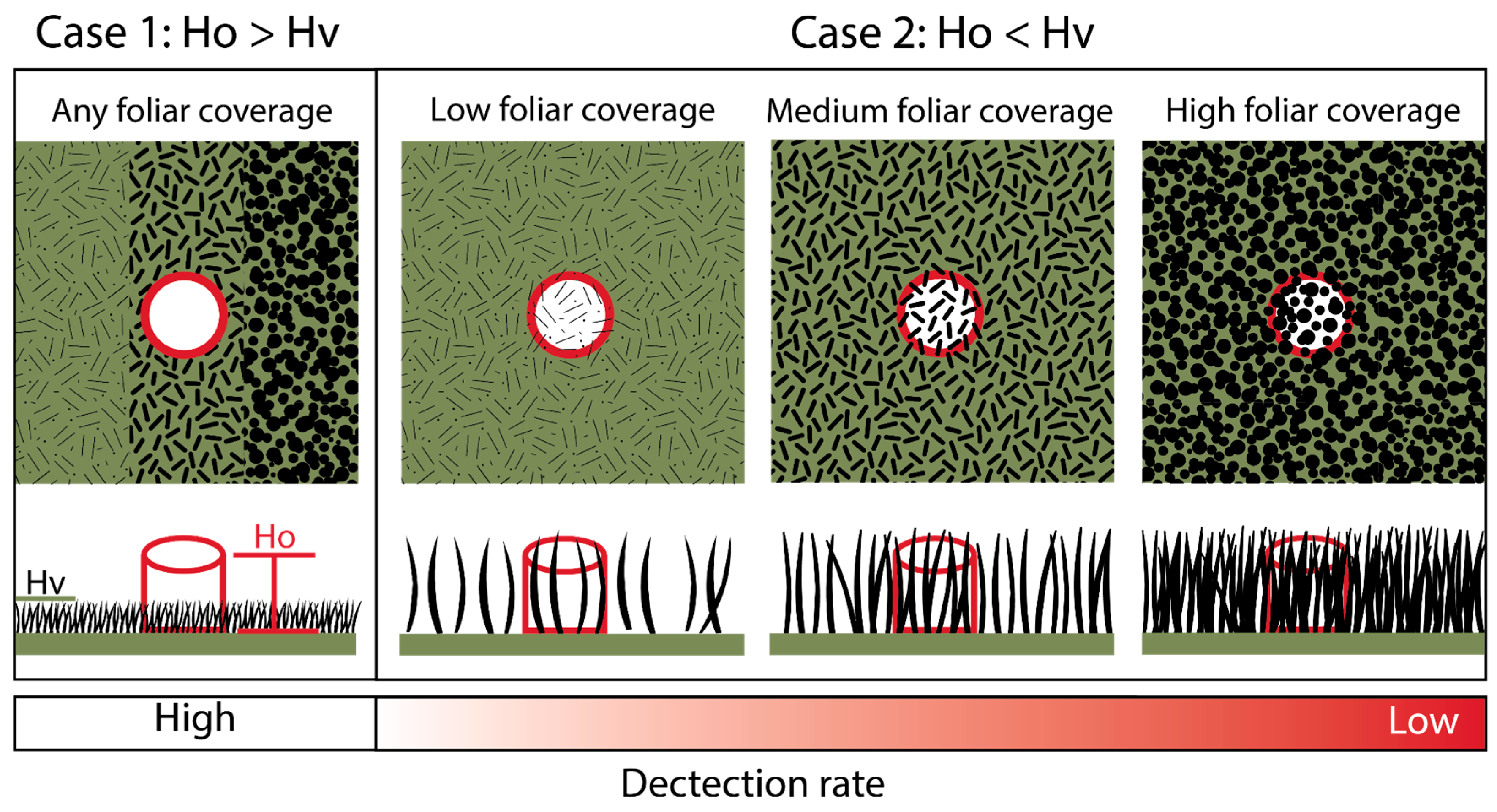
Figure 1. Schematics showing top and side views for different scenarios of an object (red outline) lying in vegetation. The left panel shows the height of the object (Ho) is greater than the vegetation height (Hv); the right panel shows the object is of similar height as the vegetation with different foliar coverage densities. The detection rate decreases from left to right.
Remotesensing 16 02046 g001
Figure 2. Sample base images of synthetic imagery with the PFM-1 with 0% occlusion. PFM-1 mines are located inside of the black boxes.
Remotesensing 16 02046 g002
Figure 3. Increasing amounts of synthetic occlusion increase width, length, and density over the PFM-1.
Remotesensing 16 02046 g003
Figure 4. The top panel shows the original orthomosaics, the middle panel shows the DSM-derived vegetation height, and the bottom panel shows the DSM-derived foliar cover >2 cm for an inert minefield with 100 landmines and UXO.
Remotesensing 16 02046 g004
Figure 5. Visualization of the experimental setup for creating a validated reference vegetation height and foliar cover dataset. (A) displays the experiment in an orthomosaic. (B) exhibits the Digital Surface Model (DSM), followed by (C) showcasing the ground-truthed maximum vegetation height per column, followed by (D) the SfM-modeled maximum vegetation height per column. On the right side, (E) presents vegetation coverage thresholded by color, representing the validated reference data for heights exceeding 10 cm. Further, (F) depicts the validated reference data foliar cover and (G) the SfM-modeled foliar cover exceeding 10 cm.
Remotesensing 16 02046 g005
Figure 6. Average recall (detection) values per bin of percent occlusion. The dots are sized by the number of observations, with the average number of observations per bin being 100 (shown in Supplemental Figure S1).
Remotesensing 16 02046 g006
Figure 7. This plot shows the uncertainty due to vegetation occlusion for the PFM-1 landmine. The golden bar shows the uncertainty from the pre-trained deep learning model. Note the recall of a pre-trained model and the uncertainty due to vegetation will vary dependent on the specific task and training dataset.
Remotesensing 16 02046 g007
Figure 8. This plot shows the correlation between the mean score of a prediction by a YOLOv8 machine learning model and the binned recall colored by percent occlusion.
Remotesensing 16 02046 g008
Figure 9. The gray line is the modeled sigmoid curve for binned recall as a function of percent occlusion for the main dataset. The orange, green, and blue dots represent the binned recall for the width, density, and length variable datasets, respectively. The dots are sized by values, with smaller dots representing smaller values of each variable.
Remotesensing 16 02046 g009
Figure 10. Orthomosaics of eight different environments used to assess the detection rate model. Inert landmines and UXO (small red boxes) were placed in all these environments for this study. The environments include (A) tarp, (B) dirt, (C) salt-flat (D) gravel, (E) grass and dirt (FH) medium height vegetation environments.
Remotesensing 16 02046 g010
Figure 11. Shows an example of extracting Hv (B) and Fcover (C,D) for an orthomosaic of an inert minefield (A).
Remotesensing 16 02046 g011
Figure 12. This figure plots the field data machine learning detection rates versus the predicted detection rates from our model for the inert minefield datasets. Each point is the 30-value rolling recall, mean sorted by modeled detection rate (‘detectability’).
Remotesensing 16 02046 g012
Figure 13. The recall rolling mean from the minefields plotted against the DSM-derived foliar cover >2 cm. Each point is the 30 value rolling mean for the recall, sorted by the UAV detection rate method.
Remotesensing 16 02046 g013
Figure 14. (A) shows the validated reference vegetation height compared to the modeled vegetation height. (B) shows the validated reference foliar cover compared to the modeled foliar cover. Both are fit by a linear least squares error regression.
Remotesensing 16 02046 g014
Figure 15. Workflow diagram, detailing all processing steps and components to create the detection rate maps in this study [18]. The italic numbers on the bottom left of the panels refer to the section number in the text describing that step.
Remotesensing 16 02046 g015
Table 1. Extracted mean and standard deviation vegetation height, foliar cover, detectability for objects that are 4 cm tall, number of UXO/landmines detected, and number of total UXO/landmines for the inert minefield environments.
EnvironmentHv Mean (cm)Hv
Stdv (cm)
Hv 0.95
(cm)
Hv
0.05
(cm)
Fcover ≥ 4 cm MeanFcover ≥ 4 cm
Std
Detectability (%) Mean for 4 cm ObjectDetectability (%) Std for 4 cm ObjectNumber of UXO DetectedTotal Number of UXO
(A)Tarp0.880.501.430.440.612.7499.120.637175
(B)Dirt0.740.882.020.141.363.3499.110.8095100
(C)Gravel1.221.142.880.551.623.1699.090.706075
(D)Salt flats1.091.363.750.143.815.3999.021.012530
(E)Farm field6.241.548.734.214.242.5398.390.726072
(F)Grass + dirt3.333.9410.880.395.597.7297.796.4877100
(G)Grass + dirt (2)3.413.8911.220.417.839.8996.728.928399
(H)Flower field13.258.8732.215.0120.0412.8981.0223.3665100
(I) High vegetation12.389.5131.192.2919.617.6477.9129.955100
Disclaimer/Publisher’s Note: The statements, opinions and data contained in all publications are solely those of the individual author(s) and contributor(s) and not of MDPI and/or the editor(s). MDPI and/or the editor(s) disclaim responsibility for any injury to people or property resulting from any ideas, methods, instructions or products referred to in the content.