Fusion of Google Street View, LiDAR, and Orthophoto Classifications Using Ranking Classes Based on F1 Score for Building Land-Use Type Detection

Abstract

Building land-use type classification using earth observation data is essential for urban planning and emergency management. Municipalities usually do not hold a detailed record of building land-use types in their jurisdictions, and there is a significant need for a detailed classification of this data. Earth observation data can be beneficial in this regard, because of their availability and requiring a reduced amount of fieldwork. In this work, we imported Google Street View (GSV), light detection and ranging-derived (LiDAR-derived) features, and orthophoto images to deep learning (DL) models. The DL models were trained on building land-use type data for the Greater Toronto Area (GTA). The data was created using building land-use type labels from OpenStreetMap (OSM) and web scraping. Then, we classified buildings into apartment, house, industrial, institutional, mixed residential/commercial, office building, retail, and other. Three DL-derived classification maps from GSV, LiDAR, and orthophoto images were combined at the decision level using the proposed ranking classes based on the F1 score method. For comparison, the classifiers were combined using fuzzy fusion as well. The results of two independent case studies, Vancouver and Fort Worth, showed that the proposed fusion method could achieve an overall accuracy of 75%, up to 8% higher than the previous study using CNNs and the same ground truth data. Also, the results showed that while mixed residential/commercial buildings were correctly detected using GSV images, the DL models confused many houses in the GTA with mixed residential/commercial because of their similar appearance in GSV images.

1. Introduction

Building land-use type is valuable information for municipalities to assess flood damage and estimate the number of exposed people during or after the flood event, but this information is either unavailable or not in a standard format [1]. The traditional method for collecting building land-use type information is ground surveying, which is labor-intensive. Some studies in the literature addressed this issue by automating this task using machine learning and earth observation data. Belgiu et al., 2014, used light detection and ranging (LiDAR) data to categorize the buildings into residential/small, factory/industrial, and apartments [2]. First, building footprints were extracted, and four kinds of features related to extent, shape, height, and slope were computed for each building footprint. Then, random forest (RF) classifier and some IF/THEN rules based on the building type ontology were applied to produce the final building type classification map. The results showed that although a high F1 score, about 98%, was achieved for residential/small buildings, the F1 scores for factory/commercial buildings and apartments were considerably lower, about 51% and 60%, respectively. Lu et al., 2014, used LiDAR data for building land-use type classification. They applied three feature types: (1) the basic statistical features such as minimum, maximum, and standard deviation computed on the first and last return pulses; (2) the shape attributes such as length, width, and length-to-width ratio; (3) the spatial relationship between buildings together and between buildings and other landscape features [3]. Wurm et al., 2015, applied 1D, 2D, and 3D building shape attributes and a linear discriminant analysis method to classify buildings into different types, such as terraced houses/row houses, and detached/semi-detached. The results showed that shape features are unsuitable for discriminating similar building types, including perimeter block development and block development [4]. Although LiDAR can give a valuable source of information about building geometric features, which can help classify buildings into residential/commercial, it does not give any spectral information, which can be helpful when discriminating other types of buildings. Orthophotos can provide spectral information, and the simultaneous use of LiDAR and orthophotos can improve identification of land-use type of buildings and reduce the chance of commission and omission errors. Meng et al., 2012, used LiDAR, aerial images, and a road network map to discriminate residential buildings from other types of buildings in Austin City, Texas using a C4.5 classification algorithm [5]. The results were compared with the field survey data, and the accuracy of about 81% was achieved for residential buildings.

Machine learning algorithms are a great choice when we have no prior assumption on the data distribution and can be used for various tasks, including multivariate non-linear non-parametric regression, supervised classification, and unsupervised classification [6]. When doing supervised classification, we need a dataset, referred to as train data, large enough to span the parameter space as much as possible. In the remote-sensing data context, supervised classification refers to when labeled data exists on the class membership of single pixels [7]. These data are used to generalize the model to the whole image. Unsupervised classification is when the training step is skipped, and the image is partitioned into different parts based on the spatial or spectral characteristics of the input image. These tasks can be achieved using different algorithms, such as neural networks, support vector machines, decision trees, and random forests.

While previous studies were extensively focused on using machine learning and deep learning (DL) algorithms for building footprint extraction [8,9,10,11,12], recent efforts have been made for building land-use type classification using earth observation data. Xie and Zhou, 2017, extracted features from high-resolution satellite images at multiple resolutions using an extended multiresolution segmentation (EMRS) algorithm and classified buildings into different functionality types with a soft classification using a back propagation (BP) network [13]. The overall accuracy improved by 19.8% compared with a single-resolution segmentation space using a hard classification with the BP network. Huang et al., 2022, created a building roof type and functionality dataset from high-resolution satellite images for Beijing and Munich Cities [14]. They examined DL-based segmentation algorithms, including mask R-CNN, cascade mask R-CNN, SOLOV2, and QueryInst, and achieved average precision at intersection over union = 0.5 (AP_0.5) of 23.5, 25.5 for Beijing and Munich Cities, respectively. Additionally, Google Street View (GSV) images have been used for building land-use type classification. Wang et al., 2017, used AlexNet to classify GSV images and achieved an overall test accuracy of about 90% on non-independent test data [15]. Zhang et al., 2017, used LiDAR, high-resolution orthophotos, and GSV images for building land-use classification of an area in New York City, USA. It was concluded that although the overall accuracy did not improve significantly after using GSV images, the mixed commercial and residential class accuracy improved by 10% [16]. Kang et al., 2018, used convolutional neural networks (CNN) to classify buildings into apartments, churches, garages, houses, industrial, office buildings, retail, and roofs using façade information from GSV images. Four CNNs were tested, including AlexNet, visual geometry group with 16 convolutional layers (VGG16), and residual network with 18 (ResNet18) and 34 (ResNet34) deep layers. The best model was VGG16 based on F1 score [17]. Al-Habashna, 2022, used GSV images and CNNs for building land-use type classification. The models used in this study were VGG16, ResNet18, ResNet34, and residual network with 50 deep layers (ResNet50). The overall accuracies achieved were up to 78% when the train and test were from the same city, and up to 69% when the train and test data were from different cities [1]. Laupheimer et al., 2018, used GSV images to classify buildings as commercial, hybrid, residential, special use, and under construction using four CNN models, VGG16, VGG19, ResNet50, and InceptionV3. The highest overall accuracy was achieved using InceptionV3, with a value of 64% [18]. Wu et al., 2023, used GSV and OSM land-use information to estimate mixed land-use types throughout New York City. The image and text information were imported into two separate encoders, and the dot product of the resultant image and text embeddings was calculated as a similarity measure. The focus of this study was more on ground land-use type detection rather than building land use [19]. In another similar study, a CNN called Conv-Depth Block Res-Unet was proposed for land-use classification in three metropolitan areas in Korea. The proposed method combined convolution and depth-wise separable convolutions and achieved an overall accuracy of 83.7% on test samples. Although the proposed method achieved high overall accuracy, and the model outperformed existing CNNs, including DeepLab V3+, ResUnet, ResASPP-Unet, and context-based ResUnet, the classification maps were not detailed in terms of building land-use type [20].

Some previous studies used the fusion of GSV, LiDAR, and aerial images for building land-use type classification. For example, Hoffmann et al., 2019, fused aerial and GSV images for classifying buildings into commercial, industrial, public, and residential. Three fusion methods based on DL were explored: (1) use of a single DL network pre-trained on GSV dataset (Places365) and ImageNet data; (2) using two streams of DL networks (VGG16), one for the GSV data and the other one for the aerial image—then, the fine-tuning was used for training the DL networks; (3) decision-level fusion by combining the Softmax probabilities or the classification labels directly using model blending and stacking approaches. The highest overall F1 score was for the decision level fusion with a value of 75% [21]. Cao et al., 2018, combined GSV and aerial images using the SegNet DL network. Two encoders were used for feature extraction, one for the GSV and the other for the aerial image. The extracted feature maps using the encoders were stacked and fed into the decoder part. The model was tested on the New York City aerial and GSV image dataset with an overall accuracy of up to 74% achieved after fusion. The highest per-class accuracy was for one and two-family buildings with a value of up to 84% [22].

While building land-use type classification using earth observation data has achieved high accuracies up to 85% for residential class on independent test data, the accuracies for other building types such as industrial, institutional, office building, and retail still need improvement [3,5]. To address this issue, we adopted two decision level fusion methods to combine three DL-based classifiers trained on GVS, LiDAR, and orthophotos for the building land-use type classification. The reason for selecting GSV is that it includes façade texture information. Also, LiDAR and orthophotos contain height and spectral information of buildings’ façades and roofs. We proposed a ranking decision level fusion method, which uses the F1 score metric to combine three DL-based classifiers. Another issue is the lack of building land-use type data. We used the web scraping technique to create label for building types, tested different heading angles when downloading GSV images to increase the sampling frequency, and applied a transfer learning strategy to reduce the DL model dependency to train data.

The paper outline is as follows: Section 1 presents the introduction and Section 2 includes case studies, data, and pre-processing. Section 3 discusses the DL models and the fusion methods. Results for GSV, LiDAR, orthophoto data, fusion results, and the related discussions were reported in Section 4. Finally, Section 5 presents the conclusions.

2. Materials and Methods

Three case studies were explored in this work. These areas were selected because of the ground truth data availability. The first case study included four cities in the Greater Toronto Area (GTA), Toronto, Vaughan, Richmond Hill, and Peel Region, with areas of 1829.05, 273.56, 100.79, and 1.25 square kilometers, and population densities of 3087.7, 1185, 2004.4, 1108.1 per square km. The number of occupied private dwellings reported in 2021, were 1,160,892, 107,159, 69,314, and 450,746 for Toronto, Vaughan, Richmond Hill, and Peel Region, respectively [23,24,25,26]. Figure 1 shows the extent of the cities on the OpenStreetMap (OSM) map, along with the building samples used in this study. The zoomed areas show the building footprints.

Two independent test case studies, including the Vancouver and Fort Worth Cities, were explored to make the train and validation data as separate as possible from the test dataset. Vancouver City, with an area of 115 square kilometers, holds a population density of 5249 per square km. In 2021, of 1,043,320 occupied private dwellings in Vancouver about 28%, 24.5%, 19%, 16%, 10%, 2%, 0.4%, and 0.1% were single-detached houses, apartments with less than five stories, apartments with five stories and more, apartments or flats in a duplex, row houses, semi-detached houses, movable dwellings, and other single detached houses [23]. Fort Worth City, located in Texas, US, with an area of 916.76 square kilometers, has a population density of 2677 per square mile, and 326,647 households were living in the city between 2018–2022 [27,28]. Figure 2 and Figure 3 show the orthophoto images of the test case studies and their ground truth maps.

The GSV, LiDAR, and orthophoto data for the GTA were used for training the DL models.

2.1. GSV Dataset

The building land-use type GSV image dataset created by [17] was used to train the DL algorithms. The data included 17,600 512 × 512 GSV images captured with a pitch angle of 10 degrees from cities across the U.S. and Canada, for example, Montreal, New York, and Denver. The ground truth labels for this data were extracted from OSM.

2.2. LiDAR Point Cloud, Orthophoto, and Building Footprint Dataset

Table 1. LiDAR data characteristics.

Case Study	Source	Vertical Accuracy	Point Density	Flight Height
GTA	Scholars Geo Portal	20.76 cm		6234 feet
Vancouver	Government of British Columbia	78 cm	8 points/${\mathrm{m}}^2$	1850 m
Fort Worth	Texas Natural Resources Information System (TNRIS)	21.2 cm	2 points/${\mathrm{m}}^2\ge$	6000 feet

shows the LiDAR point cloud data characteristics. The data were in 1 km × 1 km tiles in LAZ format, and the horizontal spatial reference system of the data was Universal Transfer Mercator (UTM) Zone 17N, and the datum was the North American Datum 1983 Canadian Spatial Reference System. The vertical spatial reference system was the Canadian Geodetic Vertical Datum 2013. For the Vancouver test area, the horizontal spatial reference system was UTM Zone 10N, with the North American Datum 1983. The vertical spatial reference system was the Canadian Geodetic Vertical Datum of 2013. For the Fort Worth test area, the Datum was North American Datum 1983, and the vertical spatial reference system was the North American Vertical Datum of 1988.

Table 2. Orthophoto and building footprint data characteristics.

Data	Case Study	Source	Year	Bands	Spatial Resolution
Orthophoto	GTA	Scholars Geo Portal	2018	R, G, B, and NIR	20 cm
	Vancouver	Vancouver Open Data Portal	2015	R, G, B	7.5 cm
	Fort Worth	Texas Natural Resources Information System (TNRIS)	2018–2019	R, G, B, and NIR	60 cm
Building Footprint	GTA	Statistics Canada	2019
	Vancouver	Vancouver Open Data Portal	2015
	Fort Worth	City of Fort Worth

shows orthophoto and building footprint data charactersitics for case studies.

2.3. ImageNet Data

The ImageNet dataset contains 14,197,144 annotated RGB images. The annotation was conducted manually with two approaches: (1) image-level binary labeling and (2) object-based labeling with bounding boxes around the objects. The reported annotation precision was 99.7%. The images were from six subtrees, including mammals, vehicles, geo forms, furniture, birds, and musical instruments [29]. These data have been used for training different types of CNNs. The CNN parameters trained on ImageNet data can be transferable to another classification problem.

2.4. Preprocessing

Some modifications were applied to the original GSV dataset to make it suitable for this study. The garage and roof classes were ignored, and the new mixed residential/commercial class was added. The final building land-use type classes included apartment, church, house, industrial, mixed residential/commercial (referred to as mixed r/c hereafter), office building, and retail. The addresses for the mixed r/c buildings were extracted using web scraping from real estate listing platforms, including CREXi, and LoopNet. The corresponding GSV images were downloaded using Google Application Programming Interface (API) and were added to the original GSV dataset. Then, the GSV images were divided into five folds and 500, 100, and 200 images were considered as train, validation, and test in each fold. Because of data scarcity for the mixed r/c class, the original number of samples was lower, with 45, 10, and 10 images as train, validation, and test. The imbalance data problem was resolved using data augmentation [30]. The samples in the mixed r/c class were flipped horizontally to make the number of train, validation, and test images the same as other classes (C).

The LiDAR-derived statistics, including mean, minimum, maximum, standard deviation, and range were calculated in ArcGIS Pro 3.1.41833 based on products of classified point cloud data, including first return (FR) pulse, last return (LR) pulse, intensity, and slope. Additionally, normalized digital surface model (nDSM) variance inside each building footprint was calculated because of the roof height variations among building land-use type classes. These statistics were calculated based on neighborhood analysis in a 3 × 3 window. The total number of LiDAR-derived features was 13, as listed in

Table 3. Features and their corresponding statistics extracted from LiDAR Point Cloud data. For example, mean, maximum, and standard deviation were calculated in a 3 × 3 moving window in the first return (FR) image.

Feature	Statistics
FR *	Mean
	Max
	Standard deviation
LR **	Mean
	Max
	Standard deviation
Intensity	Mean
	Standard deviation
Slope	Min
	Mean
	Standard deviation
	Range
nDSM	Variance

* First return, ** last return.

. Then, the features were clipped to the extent of each building footprint and reshaped into 512 × 512 for consistency with the GSV image size. The building land-use type labels were extracted using OSM. The number of samples in each class was made equal by over-sampling images in the minority classes and under-sampling images in the majority classes. After that, the created data were split into five folds. In each fold, 200, 40, and 60 feature bands, consisting of 13 LiDAR-derived features for each building footprint, were considered for train, validation, and testing. The OSM labels were relabeled for consistency with the GSV data. The commercial and government buildings were relabeled as office buildings. Also, the religious, educational, and military buildings were merged as institutional. Additionally, some building footprints assigned irrelevant or general labels such as construction, brownfield, grass, recreation ground, and fairground were relabeled as other. Finally, six classes of industrial, institutional, office building, other, residential, and retail were considered for further analysis. The Principal Component Analysis (PCA) transform was applied to the input LiDAR-derived features to equal the number of feature bands to the ImageNet dataset. In other words, in order to achieve fine-tuning, the original 13 features were reduced to 3 using PCA transformation.

Orthophoto images were clipped to the extent of each building footprint and reshaped to 512 × 512 to match the feature data size for GSV and LiDAR data. The images were then divided into five folds. In each fold, there were 200, 40, and 60 images considered for train, validation, and testing.

2.5. Deep-Learning Models Applied for Building Land-Use Type Classification

CNNs with pre-trained parameters have been used in the literature for classification tasks [31,32,33]. Some examples of these models are VGG16, MobileNetV2, and residual networks, such as ResNet18, ResNet34, and ResNet152. VGG 16 was selected for the GSV dataset because [17] applied this model, and the highest precision, recall, and F1 score, compared with AlexNet, ResNet18, and ResNet34, were achieved. To explore the suitability of other CNNs, MobileNetV2, ResNet152, and InceptionV3 [34,35,36,37] models were also applied to building land-use type classification. MobileNetV2 and VGG16 models were used for GSV images, and MobileNetv2, ResNet152, and InceptionV3 were tested for the orthophoto and LiDAR datasets. The parameters, including the optimizer and the initial learning rate were reported in

Table 4. DL model parameters: optimizer and initial learning rate. SGD and Adam are acronyms for stochastic gradient descent, and adaptive moment estimation, respectively.

Data	DL Model	Optimizers	Initial Learning Rate
GSV	MobilenetV2	SGD	10−1
	VGG16	SGD	10−3
Orthophoto	MobilenetV2	SGD	10−1
	ResNet152	SGD	10−2
	InceptionV3	Adam	10−3
LiDAR	MobileNetV2	SGD	10−6
	ResNet152	SGD	10−3
	InceptionV3	Adam	10−3

.

The loss function for all the DL models was set to the categorical cross-entropy. The initial learning rate in all the models was reduced exponentially with a decay rate, and decay step of 0.9 and 500, respectively. Each DL model consisted of two parts: (1) feature extractor; and (2) predictor. For all DL models, the feature extractor part was kept, and the predictor model was replaced with three layers, including the average pooling, drop out with 0.2 rate, and a Softmax function for class probability prediction. Finally, the arg max function was applied to the class probabilities, and the class with maximum probability was selected. For the MobileNetV2 model, only a Softmax function was added to the top of the feature extractor. Two scenarios were tested for training: (1) training the whole network, including the feature extractor and predictor models, referred to as training from scratch; (2) initializing the weights in the primary layers of the feature extractor with pre-trained parameters based on the ImageNet dataset and training the other layers with train data, referred to as transfer learning.

2.5.1. MobileNetV2

MobileNetV2 uses 19 residual blocks in its architecture. Each residual block consists of three layers. The first layer is a 1 × 1 convolution layer with a rectified linear Unit6 (ReLU6) activation function. The second layer includes the depthwise convolution, and the last layer is a 1 × 1 convolution layer with a linear activation function. This model has 154 layers in the feature extractor.

2.5.2. VGG Model

In VGG16, VGG stands for visual geometry group, and 16 refers to the number of convolutional layers. This model has a smaller receptive field than the earlier CNNs, AlexNet, and ZFNet [38,39]. In other words, instead of having a 7 × 7 or 11 × 11 convolution layer, VGG16 uses three layers of a 3 × 3 convolution layer but adds more depth to the network. The smaller receptive field has three advantages: (1) it makes the activation functions more discriminative and increases the network’s ability to converge faster; (2) it reduces the number of the network parameters; (3) by replacing the 7 × 7 convolution layer with three layers of 3 × 3 convolution and adding ReLU non-linearity between layers, the chance of overfitting is reduced. This model has 13 layers in the feature extractor.

2.5.3. ResNet152

ResNet152 stands for residual network with 152 deep layers, and it is deeper than its 34- or 101-layer counterparts. The main idea of residual networks is applying skip connections. It means the information flow can skip intermediate layers, and the feature maps can be connected to the following layers directly. There are two types of skip connections: (1) the solid line skip connection—this connection is for the case when the feature map does not need upscaling; (2) the dotted-line skip connection—this connection is for when the feature map should be increased in size. This upscaling is accomplished by either zero padding or a 1 × 1 convolution.

2.5.4. InceptionV3

InceptionV3 model is a variant of the inception networks, which use the inception modules in their architecture. Inception modules use convolution factorization in their structure. In other words, they replace n × n convolution layer with two layers of n × 1 and 1 × n convolutions. The convolution factorization can save computational power. The network consists of the inception, reduction modules, and the auxiliary classifier block. The reduction module is embedded into the network to avoid the representational bottleneck and reduce the computational burden. The auxiliary classifier block improves the network convergence and pushes the useful gradients to the lower layers [37]. The model has 313 layers in the feature extractor.

2.6. Fusion Methods

The building land-use type classification maps from orthophoto, LiDAR, and GSV images were combined using two fusion methods. We proposed a methodology based on ranking classes using the F1 score. The second method applied the fuzzy fusion concept to combine classification maps. The methods were explained in this section.

2.6.1. Ranking Classes Based on F1 Score

DL models for classification problems are usually evaluated using precision and recall rates. Precision for class c in a multi-class classification problem is the ratio of correctly classified samples in that specific class divided by the total number of samples classified in class c by the DL model (Equation (1)). The recall rate for class c is the ratio of correctly classified samples in that specific class divided by the total number of samples in the ground truth data for that class (Equation (2)). In Equations (1) and (2), True C is the total number of samples correctly classified in class c, False C is the total number of samples erroneously predicted in class c, and False NC is the total number of samples belonging to class c but were incorrectly predicted in other classes.

$$\mathrm{Precision}=\frac{\mathrm{True}\mathrm{C}}{\mathrm{True}\mathrm{C}+\mathrm{False}\mathrm{C}}$$

(1)

$$\mathrm{Recall}=\frac{\mathrm{True}\mathrm{C}}{\mathrm{True}\mathrm{C}+\mathrm{False}\mathrm{NC}}$$

(2)

F1 score combines precision and recall rates and takes the harmonic mean of these two indices as following:

$$\mathrm{F}1 \mathrm{Score}=\frac{2\times \mathrm{P}\mathrm{r}\mathrm{e}\mathrm{c}\mathrm{i}\mathrm{s}\mathrm{i}\mathrm{o}\mathrm{n}\times \mathrm{R}\mathrm{e}\mathrm{c}\mathrm{a}\mathrm{l}\mathrm{l}}{\mathrm{P}\mathrm{r}\mathrm{e}\mathrm{c}\mathrm{i}\mathrm{s}\mathrm{i}\mathrm{o}\mathrm{n}+\mathrm{R}\mathrm{e}\mathrm{c}\mathrm{a}\mathrm{l}\mathrm{l}}$$

(3)

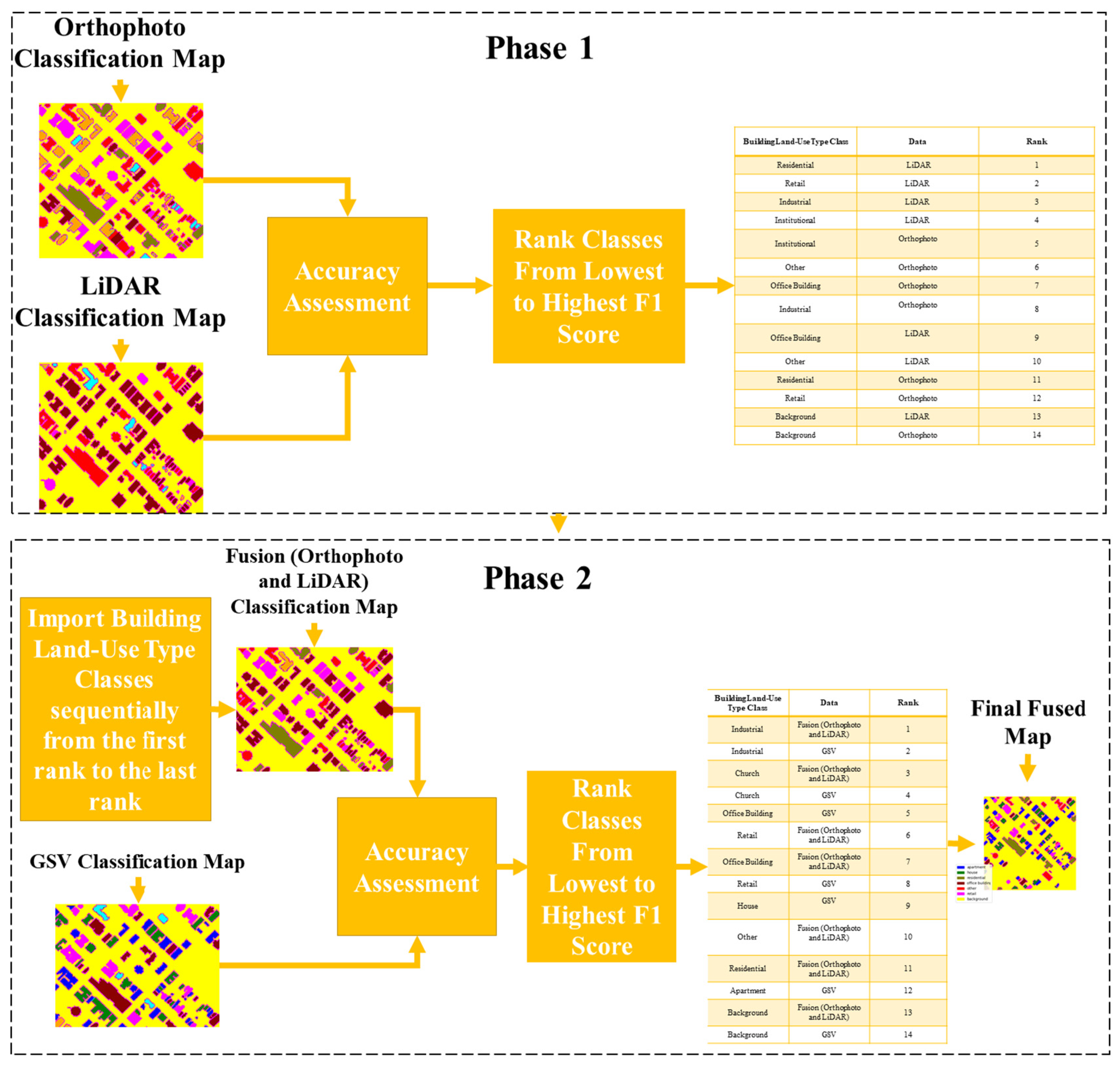
F1 score is a suitable metric for evaluating a classifier performance because it considers both accuracy and predictive power of the DL model. Hence, it is a desired metric for per class performance evaluation. When there are multiple classifiers, ranking classes based on F1 score can be a useful fusion methodology to compare classes from different information sources. We presented a methodology based on this concept to combine building land-use type classification maps from three data sources, including orthophotos, LiDAR, and GSV. This method ranks classes according to their F1 score values. The class with the lowest F1 score was ranked 1, and the class with the highest F1 score was ranked the last. The assigned rankings determine the order in which the pixels for each class are imported to the combined map. For example, if we consider the fused map as a two-dimensional empty array, first, the pixels for the class with the lowest F1 score are imported to the array, and then the pixels for the class with the second lowest F1 score are imported, and the last class imported is the class with the highest F1 score. The sequential import of pixels for each building land-use type class allows classes with low scores to be corrected by classes with higher scores. The combination process was carried out in two phases due to two reasons. Firstly, the GSV ground truth labels were in agreement with the ground truth labels in [17]. However, the LiDAR and orthophoto ground truth labels were different and were extracted from OSM. Secondly, the method was designed to be easily comprehensible to the end user. In the first phase, orthophoto and LiDAR classification maps were combined based on the ranking methodology, and in the second phase, the output from orthophoto and LiDAR maps combination was fused with the GSV classification map using the same F1 score-based ranking methodology. Please note that GSV classification maps could have been used in the first phase (after matching the labels with either orthophoto or LiDAR classification), and it should not affect the final classification results. Besides, the proposed fusion method is conducted at the pixel level. Figure 4 shows the proposed method, including phases 1 and 2.

2.6.2. Fuzzy Fusion-Based on the Gompertz Function

Assume we have M classifiers with confidence factors (CFs), $\left\{{\mathrm{C}\mathrm{F}}^1,{\mathrm{C}\mathrm{F}}^2,{\mathrm{C}\mathrm{F}}^3,\dots ,{\mathrm{C}\mathrm{F}}^{\mathrm{M}}\right\}$. These confidence factors resemble the degree of membership to a class, and their sum across different classes of a specific classifier should be equal to 1. In Equation (4), C and M refer to the total number of classes, and the total number of classifiers, respectively. Also, ${\mathrm{C}\mathrm{F}}_{\mathrm{c}}^{\mathrm{i}}$ represents the confidence factor for class c of the ith classifier.

$$\sum _{\mathrm{c}=1}^{\mathrm{C}}{\mathrm{C}\mathrm{F}}_{\mathrm{c}}^{\mathrm{i}}=1\forall \mathrm{i}=1,\dots ,\mathrm{M}$$

(4)

The fuzzy rank value for class c of the ith classifier is calculated based on the Gompertz function and by using the ${\mathrm{C}\mathrm{F}}_{\mathrm{c}}^{\mathrm{i}}$ as in Equation (5):

$${\mathrm{R}}_{\mathrm{c}}^{\mathrm{i}}=\left(1-\exp \left[-\exp \left[-2\times {\mathrm{C}\mathrm{F}}_{\mathrm{c}}^{\mathrm{i}}\right]\right]\right),\forall \mathrm{i}=1,\dots ,\mathrm{M};\mathrm{c}=1,\dots ,\mathrm{C}$$

(5)

The values of ${\mathrm{R}}_{\mathrm{c}}^{\mathrm{i}}$ lie in the range [0.127, 0.632]. The smallest value, 0.127, is analogous to the highest confidence value resulting in the lowest (best) rank.

The final decision score (FDS) for class c is calculated based on the fuzzy rank sum (FRS) for class c (Equation (6) and the complement of fuzzy rank sum (CFRS) of class c (Equation (7)):

$${\mathrm{F}\mathrm{R}\mathrm{S}}_{\mathrm{c}}=\left\{\begin{array}{l}{\mathrm{R}}_{\mathrm{c}}^{\mathrm{i}} \mathrm{if} {\mathrm{R}}_{\mathrm{c}}^{\mathrm{i}}\in {\mathrm{K}}^{\mathrm{i}}\\ {\mathrm{P}}_{\mathrm{c}}^{\mathrm{i}}, \mathrm{otherwise}\end{array}\right.$$

(6)

$${\mathrm{C}\mathrm{F}\mathrm{R}\mathrm{S}}_{\mathrm{c}}=\frac{1}{\mathrm{M}}\sum _{\mathrm{i}=1}^{\mathrm{M}}\left\{\begin{array}{l}{\mathrm{C}\mathrm{F}}_{\mathrm{c}}^{\mathrm{i}} \mathrm{if} {\mathrm{R}}_{\mathrm{c}}^{\mathrm{i}}\in {\mathrm{K}}^{\mathrm{i}} \\ {\mathrm{P}}_{\mathrm{c}}^{\mathrm{C}\mathrm{F}}, \mathrm{otherwise}\end{array}\right.$$

(7)

In the Equations above, ${\mathrm{K}}^{\mathrm{i}}$ refers to the top k ranks for class c, i.e., ranks from 1, …, k. ${\mathrm{P}}_{\mathrm{c}}^{\mathrm{i}}$ and ${\mathrm{P}}_{\mathrm{c}}^{\mathrm{C}\mathrm{F}}$ are the penalty factors imposed on class c if it does not belong to the top k ranks. ${\mathrm{P}}_{\mathrm{c}}^{\mathrm{i}}$ is set to 0.632 and is achieved by putting ${\mathrm{C}\mathrm{F}}_{\mathrm{c}}^{\mathrm{i}}=0$ in Equation (5). ${\mathrm{P}}_{\mathrm{c}}^{\mathrm{C}\mathrm{F}}$ is set to 0.

The final decision score (FDS) for class c is calculated using Equation (8) as follows:

$${\mathrm{F}\mathrm{D}\mathrm{S}}_{\mathrm{c}}={\mathrm{F}\mathrm{R}\mathrm{S}}_{\mathrm{c}}\times {\mathrm{C}\mathrm{F}\mathrm{R}\mathrm{S}}_{\mathrm{c}}$$

(8)

In the Equation above, ${\mathrm{F}\mathrm{R}\mathrm{S}}_{\mathrm{c}}$ refers to the fuzzy rank sum for class c and ${\mathrm{C}\mathrm{F}\mathrm{R}\mathrm{S}}_{\mathrm{c}}$ represents the complement of fuzzy rank sum for class c. The final predicted class of instance I of the dataset is calculated by taking the class with the minimum FDS score as in Equation (9):

$$\mathrm{c}\mathrm{l}\mathrm{a}\mathrm{s}\mathrm{s}\left(\mathrm{I}\right)=\genfrac{}{}{0pt}{}{\mathrm{a}\mathrm{r}\mathrm{g}\mathrm{m}\mathrm{i}\mathrm{n}\left\{{\mathrm{F}\mathrm{D}\mathrm{S}}_{\mathrm{c}}\right\}}{\mathrm{c}=1,2,\dots ,\mathrm{C}}$$

(9)

2.7. Accuracy Assessment

We accomplished the accuracy assessment at two different scales: (1) pixel-based; and (2) object-based. In the pixel-based accuracy assessment, precision, recall, F1 score, and overall accuracy were calculated by considering each pixel in the ground truth map as a test sample. For the object-based case, the accuracy metrics were achieved by assuming each building footprint in the ground truth map as a test sample. The Equations for the precision, recall, and F1 score were mentioned in Section 3.2.1, and Equation (10) presents the formula for the overall accuracy:

$$\mathrm{O}\mathrm{v}\mathrm{e}\mathrm{r}\mathrm{a}\mathrm{l}\mathrm{l} \mathrm{A}\mathrm{c}\mathrm{c}\mathrm{u}\mathrm{r}\mathrm{a}\mathrm{c}\mathrm{y}=\frac{{\sum }_{\mathrm{i}=1}^{\mathrm{C}}\mathrm{T}\mathrm{r}\mathrm{u}\mathrm{e} \mathrm{i}}{\mathrm{T}\mathrm{o}\mathrm{t}\mathrm{a}\mathrm{l} \mathrm{N}\mathrm{u}\mathrm{m}\mathrm{b}\mathrm{e}\mathrm{r} \mathrm{o}\mathrm{f} \mathrm{T}\mathrm{e}\mathrm{s}\mathrm{t} \mathrm{S}\mathrm{a}\mathrm{m}\mathrm{p}\mathrm{l}\mathrm{e}\mathrm{s}}$$

(10)

In the Equation above, True i, refers to the number of correctly classified samples in the ith class, and C is the total number of classes.

3. Results

This section includes the results for building land-use type classification using GSV, LiDAR, and orthophotos separately. Confusion matrices for best DL models and learning curves for different fine tuning scenarios were included in the Supplementary Materials Section. Please refer to Figures S1–S21 for further details.

3.1. Experiments on Google Street View Images

Two DL models were examined on GSV images, including MobileNetV2 and VGG16. MobileNetV2 has 154 layers in the feature extractor part, and five scenarios were examined based on the number of trained layers. In the first case, all the weights in all layers of the feature extractor network (154 layers) were trained. In the second, third, and fourth cases, 150, 100, and 50 layers out of 154 were trained, and the pre-trained weights based on the ImageNet dataset were used for the rest of the layers. In the last scenario, all the weights in 154 layers were frozen, and none of the weights in the feature extractor were trained. In other words, just the weights in the prediction layers were trained, and the weights trained on the ImageNet dataset were used in the feature extractor.

Table 5. Average accuracies across five folds and training times based on the number of trained layers; bolded numbers highlight the highest average accuracies and lowest training time for each column and model.

Model	Number of Trained Layers	Average Training Accuracy (%)	Average Validation Accuracy (%)	Average Test Accuracy (%)	Training Time (Hours)
MobileNetV2	154 (from scratch)	89.26	72.78	93.87	22.07
	150	89.63	72.17	94.28	32.37
	100	88.94	71.08	92.76	17.61
	50	87.03	71.02	93.03	25.45
	0	50.48	58.87	81.62	19.33
VGG16	13 (from scratch)	72.66	71.27	92.15	23.96
	10	72.94	71.06	92.86	29.33
	5	72.17	71.38	92.19	22.09
	0	44	54.15	74.61	22.06

shows the average training, validation, and test accuracies across five folds and the training time (in hours) for each above-mentioned transfer learning scenario. The number of trained layers in the Table refers to the number of trained layers in the feature extractor. The highest accuracies and the lowest training time have been bolded in the table. The highest overall training, validation, and test accuracies were for the MobileNetV2 with 150 trained layers, with accuracies of 89.63%, 72.17%, and 94.28%, respectively. These accuracies dropped to 50.48%, 58.87%, and 81.62% when none of the layers were trained. The training for the network with 150 trained layers took longer than other cases, about 15 h longer than the fastest model. While it was expected that the fastest training time would be for the case when all the weights were frozen, the fastest model among all MobileNetV2 models was for the network with 100 trained layers. The reason is the early stopping condition defined when training the models. Based on the condition, the algorithm would be stopped if the validation accuracy did not change more than 1% over 100 epochs. In other words, in the model for which the validation accuracy converges more quickly, the training time would be the least. Although this model was the fastest, the training, validation, and test accuracies were about 0.5%, 1%, and 1.5% lower than the best MobileNetV2 model.

The VGG16 model has 13 layers in the feature extractor part, and four transfer learning scenarios were explored. In the first scenario, all the layers in the feature extractor were trained, and in the second and third scenarios, 10 and 5 layers out of 13 were trained, respectively. The weights for the rest of the layers were kept frozen. In the last scenario, all the weights were kept frozen, and pre-trained weights based on the ImageNet dataset were used. The fastest VGG16 model, with a training time of 22.06 h, was the model in which the whole parameters were kept frozen. This result can be justified based on the lower number of trainable parameters in this network compared with other VGG16 transfer learning cases. The highest train and test accuracies, with values of 72.94% and 92.86%, were for the model with 10 trained layers. Similar to MobileNetV2, the best model in terms of test accuracy, resulted in the highest training time, 29.33 h, about 7 h longer than the fastest VGG16 model. All the average accuracy indices dropped significantly, about 29%, 17%, and 18% for train, validation, and test accuracies after freezing the whole weights in the feature extractor and using the pre-trained weights based on the ImageNet dataset.

Based on Table 5, the train and validation accuracies were 4–30% lower than test accuracy because internal cross validation was applied for accuracy assessment. This means the test data come from the same population as the train and validation data. To combat this issue, the experiments were repeated on independent test data from GTA.

Examining the Generalization Ability of DL Models Trained on GSV Images for the Greater Toronto Area

The generalization ability of the trained models was examined on an independent test dataset created for the GTA. The images were extracted from real-estate websites using the web scraping technique. These websites included LoopNet, Royallepage, and Remax. There was no image available for some addresses on the website. In these cases, the GSV images were used and downloaded using Google API. When downloading the GSV images, heading angles of 0, 90, 180, and 270 degrees and fields of view (FOV) of 22.5, 45, and 90 degrees were traversed to expand the GTA database. The extra images created using this technique were labeled based on Google Maps and street view inspection. The labels for other images were extracted from the above-mentioned real-estate websites. There was no building land-use type information available on the Remax website, so the labels were exploited from the OSM.

Table 6. Number of images in each class for GTA dataset.

Class	Number of Images
Apartment	149
House	465
Industrial	95
Mixed r/c	9
Office building	28
Retail	63

shows the number of images for each class.

Based on the test accuracies in the previous section, the best MobileNetV2 and VGG16 models were selected for building land-use type prediction for GTA. Figure 5 shows the building land-use type classification results for GTA using MobileNetV2.

Based on Figure 5, many houses were misclassified as churches. The reason for this confusion is the similarities between the two classes in GSV images. Another type of building rarely discriminated from the house because of the similar appearance was mixed r/c. For example, Figure 6 shows some houses in GSV images misclassified as mixed r/c. On the first row, the images show the houses having a similar appearance (sloped roof between the first and second floor and some windows on the second floor) to the mixed r/c image in the second row.

It is important to take into account that the accuracy values presented in Section 3.1 (Table 5) may not accurately represent the confusions mentioned above. This is because the results were obtained using GSV images, which differ from the real estate website images used for evaluation. Although the images from real estate websites used for accuracy assessment in this section may appear similar to GSV images visually, they may have inconsistent image characteristics as they are from a different source.

3.2. Experiments on LiDAR-Derived Features

Because of the limitations of building land-use type detection using GSV images, for example similarities between apartments, and office buildings, and houses to churches in a GSV image, we also explored the building land-use type classification using LiDAR and orthophoto images. The results of the analysis are reported in Section 3.2 and Section 3.3.

3.2.1. Influence of DL Model and Learning Rate on Building Land-Use Type Detection Accuracies When Training Models from Scratch

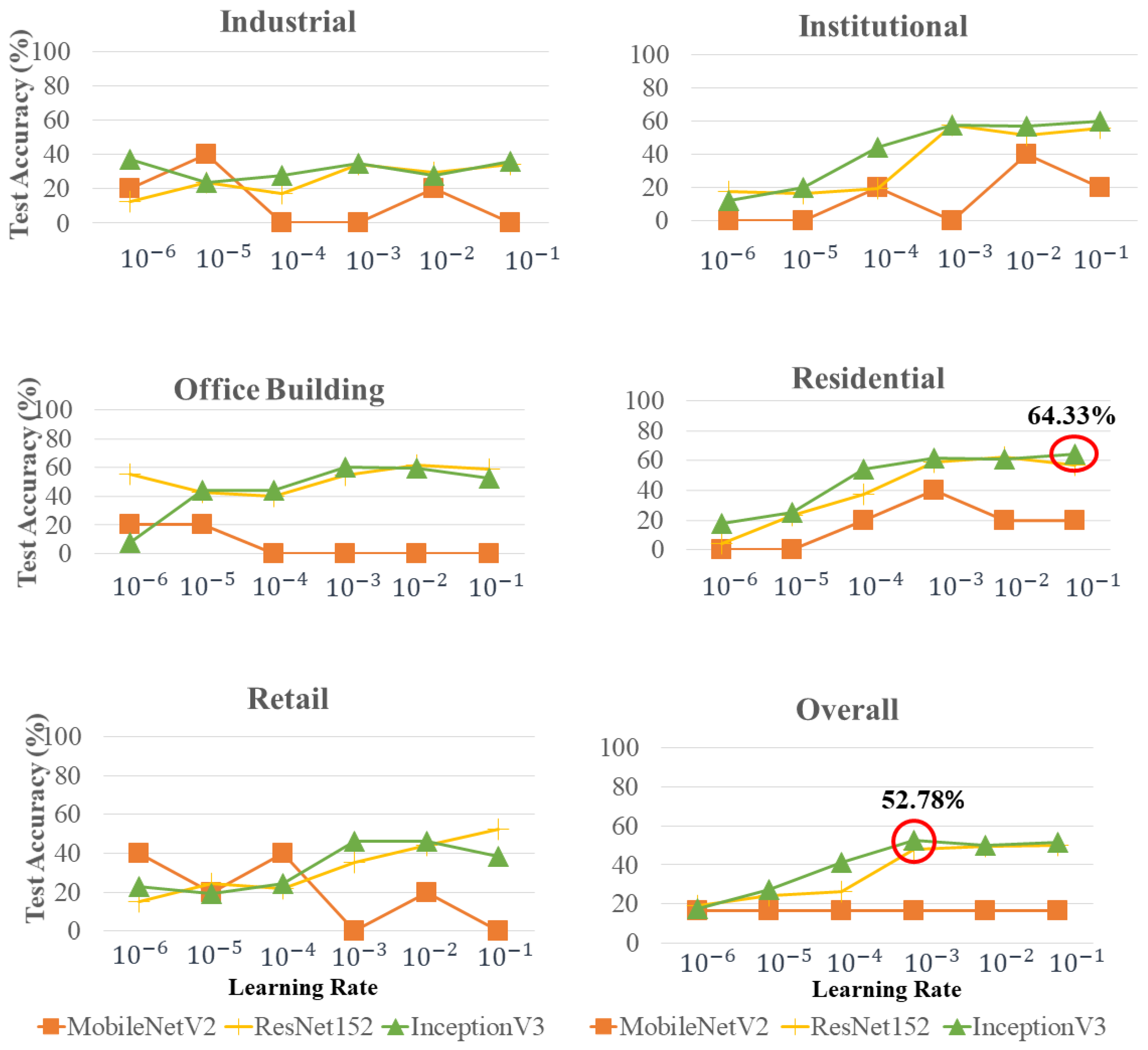
Three DL models were tested for building land-use type classification using LiDAR-derived features, including MobilenetV2, ResNet152, and InceptionV3. For each model, different learning rates, including, 10⁻⁶, 10⁻⁵, 10⁻⁴, 10⁻³, 10⁻², and 10⁻¹ were explored to find the suitable value for building land-use type classification. Two scenarios were tested for training, including training from scratch and transfer learning.

Figure 7 shows the results for each DL model when training from scratch. InceptionV3 generally achieved superior performance compared with other DL methods. The classification accuracies for residential buildings were higher than other building types, with a maximum accuracy of 64.33% when using InceptionV3 and setting the learning rate to 0.1. The building land-use type classification using LiDAR-derived features generally resulted in lower accuracies than GSV and orthophotos.

Based on accuracies for training from scratch, the DL model with the highest overall accuracy, the InceptionV3, was selected for transfer learning. Different numbers of trained layers, including 50, 100, 150, 200, 250, and 300 were examined for building land-use type classification, but transfer learning was not successful on LiDAR data, and all accuracies fell below 50%. Hence, DL models trained using the transfer learning strategy were not used in the fusion part.

3.2.2. LiDAR Building Land-Use Type Classification Maps

Figure 8 shows the ground truth and LiDAR classification maps for Vancouver. Many apartments were classified as office buildings using LiDAR data because of the height and intensity similarity backscattered from building façade between these two building types. Also, some building footprints were merged into the background because of the highest F1 score achieved for this class. There are some inconsistencies between building footprints in the ground truth and LiDAR classification maps because of the time difference between ground truth building footprint data and building footprint data used for feature extraction and classification.

Figure 9 demonstrates the ground truth and LiDAR classification maps for Fort Worth. Similar to the Vancouver case study, some apartments were classified as office buildings (highlighted with red rectangles). On the other hand, there exist few office buildings correctly detected using LiDAR data (highlighted with green rectangles).

3.3. Experiments on Orthophoto Images

This section presents the building land-use type classification accuracies when using orthophoto images.

3.3.1. Influence of DL Model and Learning Rate on Building Land-Use Type Detection Accuracies When Training from Scratch

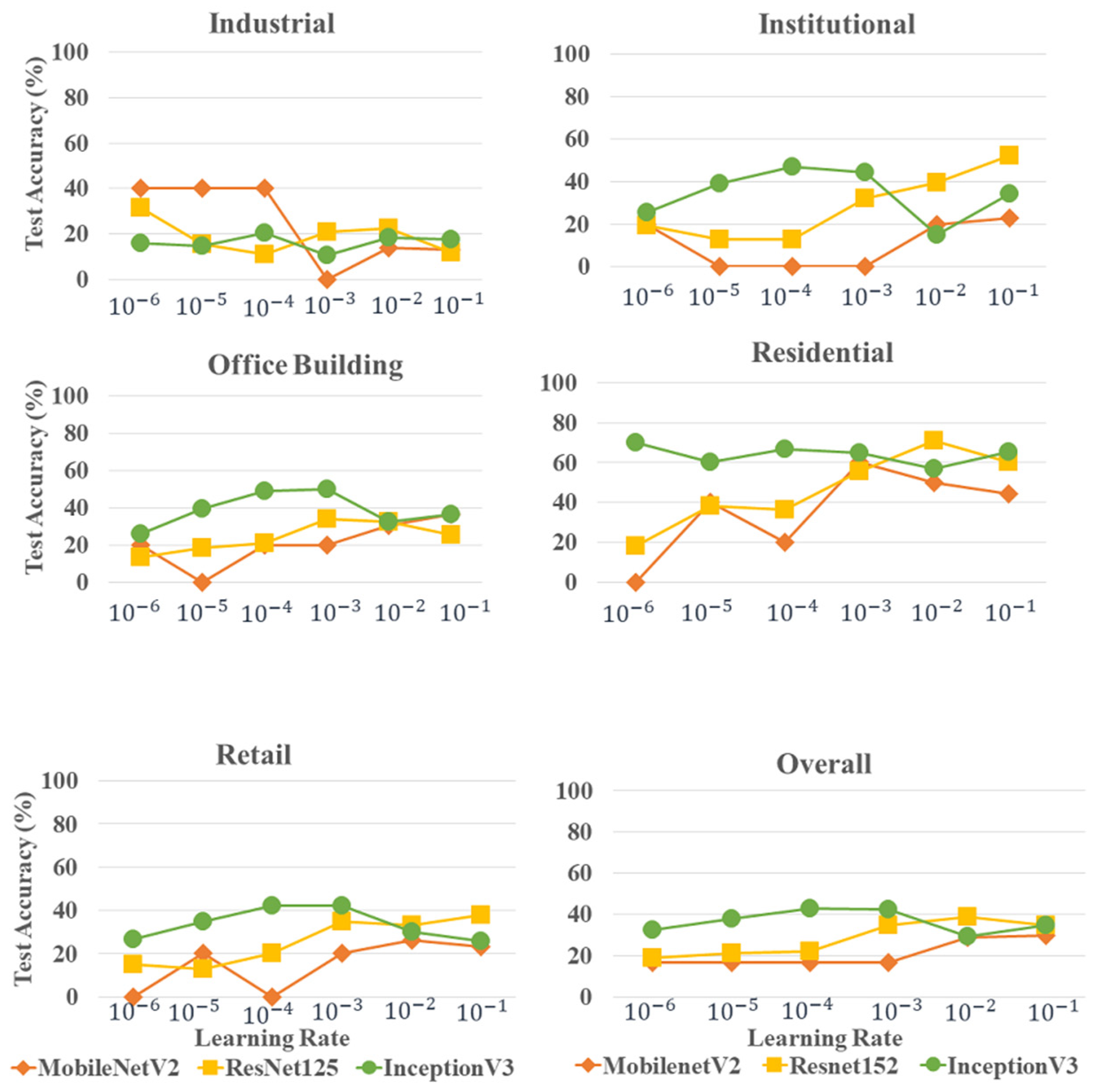
Figure 10 shows the orthophoto results with learning rates, 10⁻⁶, 10⁻⁵, 10⁻⁴, 10⁻³, 10⁻², and 10⁻¹, when training all the parameters. The figure shows that the model performance depends on the learning rate parameter significantly. The highest accuracy was for the residential class, with 71% accuracy when using the ResNet152 model with a learning rate of 10⁻². This result was about 7% higher than LiDAR-derived features. The second highest accuracy was for the InceptionV3 model, with an accuracy of 70% for the residential class when setting the learning rate to 10⁻⁶.

3.3.2. Influence of DL Model and Learning Rate on Building Land-Use Type Detection Accuracies When Using Transfer Learning

Transfer learning strategy was also examined on the orthophoto dataset, and the results are shown in Figure 11. The transfer learning strategy was more efficient than LiDAR case because of the spectral similarity (RGB bands) between ImageNet data and orthophoto images. When training 150 layers, with learning rate 10⁻³, the accuracy of 81.33% was achieved for residential class. The worst performance was for the case of using the default parameters [37].

3.3.3. Orthophoto Building Land-Use Type Classification Maps

Figure 12 shows the ground truth and orthophoto classification maps for Vancouver. Apartments and houses were classified as industrial, retail, and other. A few retail buildings, highlighted with green rectangles, were successfully classified using orthophoto data.

Figure 13 depicts the ground truth and orthophoto classification maps for Fort Worth. Same as the Vancouver case study, there were a few buildings correctly detected using orthophoto data. These building footprints were highlighted using green rectangles. Most office buildings in Fort Worth were classified as retail, church, and other using orthophoto images.

4. Discussion

This section includes discussions on model training time and the fusion methods applied.

4.1. Deep-Learning Models Training Time

DL algorithms have millions of parameters, and training this huge number of parameters is time-consuming. Finding the trade-off between training time and accuracy has always been one of the challenges in DL models. Figure 14 shows the training time when training all the parameters for LiDAR-derived features and orthophoto images with learning rates of 10⁻⁶, 10⁻⁵, 10⁻⁴, 10⁻³, 10⁻², and 10⁻¹. Most models had a training time of less than 1.5 h, except ResNet152 trained on orthophoto images, with training time fluctuating between 2–3 h. DL model, GPU type, optimizer, and input dataset contribute to the training speed. The most time-consuming model was ResNet152 on orthophoto images because the model has 60.4 million parameters, the highest among the three models. The least training time was for MobileNetV2 on both LiDAR and orthophoto data because this model has the lowest number of parameters compared with InceptionV3 and ResNet152.

4.2. Fusion of Orthophotos, LiDAR, and GSV

The GSV, LiDAR, and orthophoto classification maps were fused to improve the generalization ability of GSV classifications. We examined two fusion methods: (1) ranking classes based on the F1 score; and (2) fuzzy fusion based on the Gompertz function [17] mentioned in Section 3.3.1 and Section 3.3.2. Two ground truth data used by [17] were tested in this section. The dataset included building land-use type labels for Vancouver and Fort Worth. The ground truth dataset has been shown in Figure 15. Most buildings in the Vancouver and Fort Worth ground truth datasets were apartments and office buildings, respectively.

The results in Figure 16 show the precision and recall rates for each building land-use class in the City of Vancouver, as well as the overall accuracy. In this experiment, the building types of church and industrial were not included because they had very few samples in the ground truth, and none of the classifiers were able to detect these building types before or after fusion.

The proposed method was able to improve the precision of house detection by 36% compared to GSV, achieving a value of 41%. In addition, the proposed method was able to detect buildings with the other building land-use class with precision and recall rates of 13% and 26%, respectively, while GSV was not able to detect them at all. The background class’s recall rate for the proposed method was 91%, which was 2% higher than the corresponding value for the GSV result. Overall accuracy also improved by 1% after using the proposed method, achieving a value of 67%.

Although the proposed method showed superior performance for the background class’s recall rate, with 6% higher rate than the fuzzy fusion method, and 13% and 26% precision and recall rates for the other class, respectively, the fuzzy fusion method generally showed better performance for pixel-based accuracy indices in the City of Vancouver. The fuzzy method showed better performance for the apartment and house classes, with 4% and 32% improvement in precision and recall rates, respectively. Additionally, precision and recall rates for the retail class improved after using the fuzzy fusion method, with values of 16% and 42%, respectively. Another improvement when using the fuzzy fusion method was in terms of background precision, which improved from 81% to 87%. Furthermore, the overall accuracy also improved by 3%, achieving a value of 70% when using the fuzzy fusion method.

Object-based per-class precision, and recall, as well as overall accuracies in the City of Vancouver are presented in Figure 17. The office building class was excluded from the analysis due to the absence of building footprints in both pre- and post-fusion stages. Similarly, the background class was not considered in the object-based analysis, as it is a pixel-based class and does not include any building footprint. After applying the proposed fusion method, there was a 21% and 11% increase in precision and recall rates for the apartment class, respectively, resulting in values of 72% and 39%. The proposed method also led to a 2% and 17% improvement in the precision and recall rates of the house class, respectively. However, the fusion method had an adverse effect on the other class, with no building footprint being classified under this category. The proposed method did not affect the performance of the retail class, and no buildings were detected in this group before or after fusion. Overall accuracy was enhanced by 20% after applying the proposed fusion method, with a more significant increase compared to the 1% improvement in the pixel-based overall accuracy.

Generally, the fuzzy fusion method resulted in a higher performance than the fuzzy method in terms of object-based accuracy indices. For example, the recall rate for the apartment class was 24% higher than the proposed method and achieved a value of 63%. Also, the precision and recall rates for the house class were 12% and 43% higher than the proposed method when using the fuzzy fusion algorithm, with values of 39% and 63%. However, the proposed method had a better performance than the fuzzy fusion method in terms of the apartment class’s precision. When using the proposed method, the index was higher by 33%. Although both fusion methods degraded the other class performance, fuzzy fusion improved the retail class’s precision and recall rates. Before fusion and when using the proposed method, no building footprint was detected in the retail class. However, when using fuzzy fusion, precision and recall rates of 35% were achieved. Because of the improvements in class performance when using the fuzzy fusion method, the overall accuracy when using this method was 2% higher than the proposed algorithm.

Figure 18 shows the pixel-based per-class precision and recall indices along with overall accuracies in Fort Worth City. The proposed fusion method was more effective than GSV in improving several accuracy indices. Specifically, the proposed method achieved precision and recall rates of 9% for the industrial building class, which GSV could not detect. Furthermore, the precision and recall rates for the office building class improved by 2% and 8%, respectively, with values of 43% and 38% being achieved. Additionally, the background class recall rate improved by 2% after using the proposed method, resulting in a value of 89%. Finally, the pixel-based overall accuracy increased by 3% after the proposed method was used, resulting in a value of 75%.

In terms of comparing the proposed fusion method with fuzzy fusion, the fuzzy fusion technique was unable to detect any pixel in the industrial class. However, the proposed fusion method achieved precision and recall rates of 9% and 10%, respectively. Moreover, the recall rates for the office building and background classes were higher by 35% and 2%, compared to the fuzzy method. Overall, the proposed method improved the pixel-based accuracy by 7% with a value of 75% achieved, whereas the overall accuracy index of fuzzy fusion was even lower than GSV classification. The 75% overall accuracy was 1% higher than Cao et al., 2018, fusing GSV and aerial images. Although the proposed method generally showed better performance than fuzzy fusion, there were instances where fuzzy fusion demonstrated superior performance. For instance, the precision of the office building class was 9% higher with a value of 52% achieved compared to the proposed method. Furthermore, while GSV and the proposed method could not detect any pixels in the other and residential classes, fuzzy fusion achieved 80% precision and 14% recall rates for the other class and 7% precision and 31% recall rates for the residential class. In the retail class, fuzzy fusion achieved higher precision and recall rates by 2% and 44%, respectively. Finally, fuzzy fusion method achieved a higher precision of 89% for the background class, which was 3% higher than the proposed method.

The object-based precision, recall rates, and overall accuracy for Fort Worth are depicted in Figure 19. After using the proposed method for fusion, there were notable improvements in the precision and recall indices for the office buildings class, with 18% and 46% increases resulting in values of 38% and 51%, respectively. The retail class also experienced 1% and 9% increases in precision and recall rates after the fusion process. Finally, the overall accuracy had a 10% improvement, resulting in a value of 25%. When compared with fuzzy fusion, the proposed method yielded even better results. For instance, the office building class precision and recall rates both experienced a 5% and 48% increase, respectively. Additionally, the proposed method achieved a higher precision rate for the retail class by 4%. On the other hand, the overall accuracy for fuzzy fusion was lower, with a value of 7%, when compared to both GSV and the proposed method.

Fuzzy fusion and F1 score fusion achieved overall accuracies about 1% and 8% higher than the previous study using GSV and the VGG16 model for the Fort Worth test region [17]. The method applied in our work differs from the previous study in terms of using an information fusion approach for building land-use type classification. While the previous work focused on GSV data, we combined three DL-based classifiers trained on GSV, LiDAR, and orthophotos for classification.

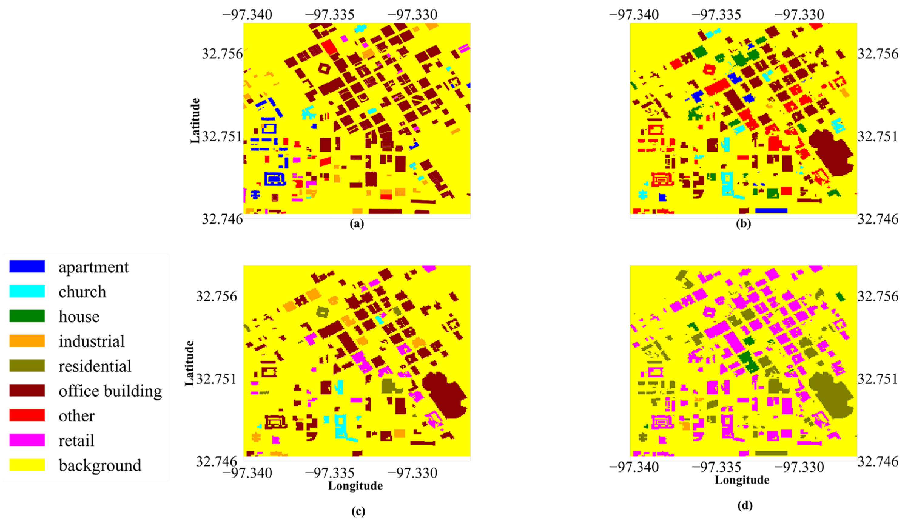
Figure 20 shows the ground truth, GSV, and fusion classification maps for Vancouver. Based on the F1 score fusion classification map (part (c)), many building footprints were merged into the background class because this class was given the highest rank over other classes. While some buildings in fusion maps were not in the ground truth map because of inconsistency between the 2015 Vancouver building footprint data and ground truth, most buildings in the fuzzy fusion map were labeled. The fuzzy fusion method faced difficulty in distinguishing between the houses and apartments classes within residential buildings due to inconsistencies between the ground truth labels for orthophoto-LiDAR and GSV images. The web scraping technique used for ground truth creation in GSV image classification could not be applied for LiDAR and orthophoto classifications because it was not possible to find LiDAR and orthophoto data for the same address as the addresses retrieved from web scraping. Although the proposed method did not show significant improvement compared to GSV, it outperformed the fuzzy fusion method by accurately classifying buildings into houses and apartments. The classification maps in Figure 21 show building land-use type classification results in Fort Worth City. After comparing the building land-use type classification maps generated using GSV images and the proposed algorithm, some improvements can be observed after the fusion. For instance, in the GSV map, there was one building footprint on the top and three small building footprints on the right (rectangles) that were incorrectly detected as other or industrial, but the proposed method correctly classified them as office buildings. Additionally, while fuzzy fusion mislabeled many office buildings as retail, the proposed method was able to correctly classify these buildings.

5. Conclusions

This study explored a detailed building land-use type classification. The building footprints were classified as apartments, houses, churches, industrial, office buildings, other, and retail. Also, mixed r/c buildings were detected using the GSV dataset. While reducing the number of classes might increase the overall accuracies, this study aimed to train models to classify buildings into more detailed land-use classes than previous studies. The other class included different land-use/land-cover types, including construction, brownfield, grass, recreation ground, and fairground, and had a significant intra-class class variability. While the intra-class variability would cause lower classification performance, the accuracies did not change significantly after excluding the other class. The building land-use type classification was accomplished using the fusion of three DL-based classifiers trained on GSV, LiDAR, and orthophoto data using the proposed F1 score fusion and fuzzy fusion methods to improve the GSV classification result. A fuzzy fusion method based on the Gompertz function was tested for combining classifiers at the decision level. The results showed that although the fuzzy method improved recall rates and overall accuracies for Vancouver, almost all accuracy indices dropped for Fort Worth City. The proposed F1 score method improved the pixel-based and the object-based precision and overall accuracies for both independent test data. In comparison among GSV, LiDAR, and orthophotos, the best test accuracy on non-independent test data was for the GSV data, but the accuracy degraded significantly after testing the DL models on the independent test data. The transfer learning method was efficient on GSV and orthophoto datasets but was not successful on LiDAR data because of inconsistency between the ImageNet data and LiDAR-derived features. MobileNetV2 and InceptionV3 models achieved the highest test accuracies for GSV, LiDAR, and orthophoto data, respectively.

References

1. Al-Habashna, A. Building Type Classification from Street-View Imagery Using Convolutional Neural Networks; Statistics Canada: Ottawa, ON, Canada, 2022; Available online: https://www150.statcan.gc.ca/n1/en/pub/18-001-x/18-001-x2021003-eng.pdf?st=A02HTs8U (accessed on 1 February 2024).
2. Belgiu, M.; Tomljenovic, I.; Lampoltshammer, T.J.; Blaschke, T.; Höfle, B. Ontology-based classification of building types detected from airborne laser scanning data. Remote Sens. 2014, 6, 1347–1366. [Google Scholar] [CrossRef]
3. Lu, Z.; Im, J.; Rhee, J.; Hodgson, M. Building type classification using spatial and landscape attributes derived from LiDAR remote sensing data. Landsc. Urban Plan. 2014, 130, 134–148. [Google Scholar] [CrossRef]
4. Wurm, M.; Schmitt, A.; Taubenböck, H. Building types’ classification using shape-based features and linear discriminant functions. IEEE J. Sel. Top. Appl. Earth Obs. Remote Sens. 2015, 9, 1901–1912. [Google Scholar] [CrossRef]
5. Meng, X.; Currit, N.; Wang, L.; Yang, X. Detect residential buildings from lidar and aerial photographs through object-oriented land-use classification. Photogramm. Eng. Remote Sens. 2012, 78, 35–44. [Google Scholar] [CrossRef]
6. Lary, D.J.; Zewdie, G.K.; Liu, X.; Wu, D.; Levetin, E.; Allee, R.J.; Malakar, N.; Walker, A.; Mussa, H.; Mannino, A.; et al. Machine learning applications for earth observation. Earth Obs. Open Sci. Innov. 2018, 165, 165–180. [Google Scholar]
7. Camps-Valls, G. Machine learning in remote sensing data processing. In Proceedings of the 2009 IEEE International Workshop on Machine LEARNING for Signal Processing, Grenoble, France, 1–4 September 2009; IEEE: Piscataway, NJ, USA, 2009; pp. 1–6. [Google Scholar]
8. Yan, L.; Zhang, J.; Huang, G.; Zhao, Z. Building Footprints Extraction from PolSAR Image Using Multi-Features and Edge Information. In Proceedings of the 2011 International Symposium on Image and Data Fusion, Tengchong, China, 9–11 August 2011; IEEE: Piscataway, NJ, USA, 2011; pp. 1–5. [Google Scholar]
9. Abdollahi, A.; Pradhan, B.; Gite, S.; Alamri, A. Building footprint extraction from high resolution aerial images using generative adversarial network (GAN) architecture. IEEE Access 2020, 8, 209517–209527. [Google Scholar] [CrossRef]
10. Liu, T.; Yao, L.; Qin, J.; Lu, N.; Jiang, H.; Zhang, F.; Zhou, C. Multi-scale attention integrated hierarchical networks for high-resolution building footprint extraction. Int. J. Appl. Earth Obs. Geoinf. 2022, 109, 102768. [Google Scholar] [CrossRef]
11. Rastogi, K.; Bodani, P.; Sharma, S.A. Automatic building footprint extraction from very high-resolution imagery using deep learning techniques. Geocarto Int. 2022, 37, 1501–1513. [Google Scholar] [CrossRef]
12. Yu, H.; Hu, H.; Xu, B.; Shang, Q.; Wang, Z.; Zhu, Q. SuperpixelGraph: Semi-automatic generation of building footprint through semantic-sensitive superpixel and neural graph networks. Int. J. Appl. Earth Obs. Geoinf. 2023, 125, 103556. [Google Scholar] [CrossRef]
13. Xie, J.; Zhou, J. Classification of urban building type from high spatial resolution remote sensing imagery using extended MRS and soft BP network. IEEE J. Sel. Top. Appl. Earth Obs. Remote Sens. 2017, 10, 3515–3528. [Google Scholar] [CrossRef]
14. Huang, X.; Ren, L.; Liu, C.; Wang, Y.; Yu, H.; Schmitt, M.; Hänsch, R.; Sun, X.; Huang, H.; Mayer, H. Urban building classification (ubc)-a dataset for individual building detection and classification from satellite imagery. In Proceedings of the IEEE/CVF Conference on Computer Vision and Pattern Recognition (CVPR) Workshops, New Orleans, LA, USA, 18–24 June 2022; pp. 1413–1421. [Google Scholar]
15. Wang, Q.; Zhou, C.; Xu, N. Street view image classification based on convolutional neural network. In Proceedings of the 2017 IEEE 2nd Advanced Information Technology, Electronic and Automation Control Conference (IAEAC), Chongqing, China, 25–26 March 2017; IEEE: Piscataway, NJ, USA, 2017; pp. 1439–1443. [Google Scholar]
16. Zhang, W.; Li, W.; Zhang, C.; Hanink, D.M.; Li, X.; Wang, W. Parcel-based urban land use classification in megacity using airborne LiDAR, high resolution orthoimagery, and Google Street View. Comput. Environ. Urban Syst. 2017, 64, 215–228. [Google Scholar] [CrossRef]
17. Kang, J.; Körner, M.; Wang, Y.; Taubenböck, H.; Zhu, X.X. Building instance classification using street view images. ISPRS J. Photogramm. Remote Sens. 2018, 145, 44–59. [Google Scholar] [CrossRef]
18. Laupheimer, D.; Tutzauer, P.; Haala, N.; Spicker, M. Neural networks for the classification of building use from street-view imagery. ISPRS Ann. Photogramm. Remote Sens. Spat. Inf. Sci. 2018, 4, 177–184. [Google Scholar] [CrossRef]
19. Wu, M.; Huang, Q.; Gao, S.; Zhang, Z. Mixed land use measurement and mapping with street view images and spatial context-aware prompts via zero-shot multimodal learning. Int. J. Appl. Earth Obs. Geoinf. 2023, 125, 103591. [Google Scholar] [CrossRef]
20. Yoo, S.; Lee, J.; Farkoushi, M.G.; Lee, E.; Sohn, H.-G. Automatic generation of land use maps using aerial orthoimages and building floor data with a Conv-Depth Block (CDB) ResU-Net architecture. Int. J. Appl. Earth Obs. Geoinf. 2022, 107, 102678. [Google Scholar] [CrossRef]
21. Hoffmann, E.J.; Wang, Y.; Werner, M.; Kang, J.; Zhu, X.X. Model fusion for building type classification from aerial and street view images. Remote Sens. 2019, 11, 1259. [Google Scholar] [CrossRef]
22. Cao, R.; Zhu, J.; Tu, W.; Li, Q.; Cao, J.; Liu, B.; Zhang, Q.; Qiu, G. Integrating aerial and street view images for urban land use classification. Remote Sens. 2018, 10, 1553. [Google Scholar] [CrossRef]
23. Government of Canada. Census Profile, 2021 Census of Population. Profile Table. Available online: https://www12.statcan.gc.ca/census-recensement/2021/dp-pd/prof/details/page.cfm?Lang=E&DGUIDlist=2021A00053519038&GENDERlist=1&STATISTIClist=1&HEADERlist=0 (accessed on 1 February 2024).
24. Vaughan Economic Development. 2021 Census Insights and Findings—Population and Dwellings. Available online: https://vaughanbusiness.ca/insights/2021-census-insights-and-findings-population-and-dwellings/ (accessed on 14 February 2024).
25. Government of Canada. Focus on Geography Series, 2016 Census. Available online: https://www12.statcan.gc.ca/census-recensement/2016/as-sa/fogs-spg/Facts-cd-eng.cfm?LANG=Eng&GK=CD&GC=3521&TOPIC=1 (accessed on 14 February 2024).
26. Government of Canada. Population and Dwelling Counts: Canada and Population Centres. Available online: https://www12.statcan.gc.ca/census-recensement/2016/as-sa/fogs-spg/Facts-csd-eng.cfm?LANG=Eng&GK=CSD&GC=3520005&TOPIC=1 (accessed on 30 May 2024).
27. City of Fort Worth. Chapter 1 Population Trends. Available online: https://www.fortworthtexas.gov/files/assets/public/v/1/the-fwlab/documents/comprehensive-planning/pdf-adopted/01_populationtrends.pdf (accessed on 28 February 2024).
28. United States Census Bureau. QuickFacts, Fort Worth City, Texas; Texas. Available online: https://www.census.gov/quickfacts/fact/table/fortworthcitytexas (accessed on 28 February 2024).
29. Deng, J.; Dong, W.; Socher, R.; Li, L.J.; Li, K.; Li, F.F. Imagenet: A large-scale hierarchical image database. In Proceedings of the 2009 IEEE Conference on Computer Vision and Pattern Recognition, Miami, FL, USA, 20–25 June 2009; IEEE: Piscataway, NJ, USA, 2009; pp. 248–255. [Google Scholar]
30. Chen, C.; Fan, L. Scene segmentation of remotely sensed images with data augmentation using U-net++. In Proceedings of the 2021 International Conference on Computer Engineering and Artificial Intelligence (ICCEAI), Shanghai, China, 27–29 August 2021; IEEE: Piscataway, NJ, USA, 2021; pp. 201–205. [Google Scholar]
31. Karadal, C.H.; Kaya, M.C.; Tuncer, T.; Dogan, S.; Acharya, U.R. Automated classification of remote sensing images using multileveled MobileNetV2 and DWT techniques. Expert Syst. Appl. 2021, 185, 115659. [Google Scholar] [CrossRef]
32. Kumar, A.; Abhishek, K.; Singh, A.K.; Nerurkar, P.; Chandane, M.; Bhirud, S.; Patel, D.; Busnel, Y. Multilabel classification of remote sensed satellite imagery. Trans. Emerg. Telecommun. Technol. 2021, 32, e3988. [Google Scholar] [CrossRef]
33. Liu, K.; Yu, S.; Liu, S. An improved InceptionV3 network for obscured ship classification in remote sensing images. IEEE J. Sel. Top. Appl. Earth Obs. Remote Sens. 2020, 13, 4738–4747. [Google Scholar] [CrossRef]
34. Sandler, M.; Howard, A.; Zhu, M.; Zhmoginov, A.; Chen, L.-C. Mobilenetv2: Inverted residuals and linear bottlenecks. In Proceedings of the IEEE Conference on Computer Vision and Pattern Recognition (CVPR), Salt Lake City, UT, USA, 18–23 June 2018; pp. 4510–4520. [Google Scholar]
35. Simonyan, K.; Zisserman, A. Very deep convolutional networks for large-scale image recognition. arXiv 2014, arXiv:1409.1556. [Google Scholar]
36. He, K.; Zhang, X.; Ren, S.; Sun, J. Deep residual learning for image recognition. In Proceedings of the IEEE Conference on Computer Vision and Pattern Recognition (CVPR), Las Vegas, NV, USA, 27–30 June 2016; pp. 770–778. [Google Scholar]
37. Szegedy, C.; Vanhoucke, V.; Ioffe, S.; Shlens, J.; Wojna, Z. Rethinking the inception architecture for computer vision. In Proceedings of the IEEE Conference on Computer Vision and Pattern Recognition (CVPR), Las Vegas, NV, USA, 27–30 June 2016; pp. 2818–2826. [Google Scholar]
38. Krizhevsky, A.; Sutskever, I.; Hinton, G.E. ImageNet classification with deep convolutional neural networks. Commun. ACM 2017, 60, 84–90. [Google Scholar] [CrossRef]
39. Zeiler, M.D.; Fergus, R. Visualizing and understanding convolutional networks. In Computer Vision–ECCV 2014: Proceedings of the 13th European Conference on Computer Vision (ECCV), Zurich, Switzerland, 6–12 September 2014; Proceedings, Part I 13; Springer: Berlin/Heidelberg, Germany, 2014; pp. 818–833. [Google Scholar]
Figure 1. Greater Toronto Area (GTA) case study. The color dots indicate building samples within the boundary including the cities of Toronto, Markham, Vaughan, Richmond Hill, and the Peel region. The background map corresponds to OpenStreetMap (OSM).
Remotesensing 16 02011 g001
Figure 2. Vancouver test region: (a) orthophoto image; (b) ground truth map.
Remotesensing 16 02011 g002
Figure 3. Fort Worth test region: (a) orthophoto image; (b) ground truth map.
Remotesensing 16 02011 g003
Figure 4. The graphical abstract for F1 score ranking fusion method.
Remotesensing 16 02011 g004
Figure 5. MobileNetV2 building land-use type classification result. Many houses (green dots) were misclassified as churches (cyan dots). (a) Ground truth. (b) Predicted Map.
Remotesensing 16 02011 g005
Figure 6. Houses misclassified as mixed r/c because both building types have a sloped roof between the first and second floor and some windows on the second floor: the images on the first row are houses misclassified as mixed r/c and the image on the second row is a mixed r/c building.
Remotesensing 16 02011 g006
Figure 7. Building land-use type classification accuracies for LiDAR-derived features when training from scratch and using DL models, including, MobileNetV2, ResNet152, and InceptionV3 (the red circles show the highest accuracy for the residential class with 64.33% test accuracy and the highest overall accuracy with a value of 52.78%).
Remotesensing 16 02011 g007
Figure 8. (a) Ground truth map for Vancouver. (b) LiDAR building land-use type classification map for Vancouver.
Remotesensing 16 02011 g008
Figure 9. (a) Ground truth map for Fort Worth. (b) LiDAR building land-use type classification map for Fort Worth. Red rectangles highlight apartments in ground truth maps erroneously detected as office building using LiDAR. Green rectangles show the correctly detected office buildings using LiDAR data.
Remotesensing 16 02011 g009
Figure 10. Building land-use type classification accuracies for orthophotos when training from scratch and using DL models, including, MobileNetV2, ResNet152, and InceptionV3 (the highest accuracy was for the residential class with 71% test accuracy in the best case).
Remotesensing 16 02011 g010
Figure 11. Building land-use type classification accuracies for orthophotos when using transfer learning and InceptionV3 (the red circles show the highest accuracies for the residential class with a value of about 81% and overall with a value of about 53%; the vertically dotted red line shows the number of trained layers that resulted in the highest accuracies). LR is an acronym for learning rate; Adam and RMSProp refer to the adaptive moment estimation and root mean square propagation optimizers, respectively.
Remotesensing 16 02011 g011
Figure 12. (a) Vancouver ground truth map. (b) Orthophoto building land-use type classification map for Vancouver. Green rectangles show the correctly classified retail buildings.
Remotesensing 16 02011 g012
Figure 13. (a) Fort Worth ground truth map. (b) Orthophoto building land-use type classification map for Fort Worth. Green rectangles show the correctly classified office buildings.
Remotesensing 16 02011 g013
Figure 14. Training time for DL models. T4, A100, and V100 refer to the GPU types.
Remotesensing 16 02011 g014
Figure 15. Ground truth labels for: (a) Vancouver; (b) Fort Worth.
Remotesensing 16 02011 g015
Figure 16. Pixel-based precision (blue bars), recall (orange bars), and overall accuracies (gray bars) for GSV, the proposed method, and fuzzy fusion. (a) Precision and recall indices for building land-use type classes apartment, house, office building, and others. (b) Precision and recall indices for classes retail and background, and overall accuracies.
Remotesensing 16 02011 g016
Figure 17. Object-based precision (blue bars) and recall (orange bars) for each building land-use type and overall accuracy (gray bars) indices in the City of Vancouver. The results are for GSV, the proposed fusion method, and fuzzy fusion classifications.
Remotesensing 16 02011 g017
Figure 18. Per-class pixel-based precision (blue bars) and recall (orange bars) for GSV, the proposed method, and fuzzy fusion classifications in Fort Worth City. The gray bars show overall accuracy indices for the classifications.
Remotesensing 16 02011 g018
Figure 19. Per-class object-based precision (blue bars) and recall (orange bars) for GSV, the proposed method, and fuzzy fusion classifications in Fort Worth City. Gray bars depict the overall accuracies for classifications.
Remotesensing 16 02011 g019
Figure 20. Building land-use type classification maps for Vancouver case study: (a) ground truth; (b) GSV classification map; (c) the proposed fusion method; (d): fuzzy fusion.
Remotesensing 16 02011 g020
Figure 21. Building land-use type classification maps for Fort Worth case study: (a) ground truth; (b) GSV classification map; (c) the proposed fusion method; (d): fuzzy fusion.
Remotesensing 16 02011 g021