Abstract
The recently deployed Surface Water and Ocean Topography (SWOT) mission for the first time has observed the ocean surface at a spatial resolution of 1 km, thus giving an opportunity to directly monitor submesoscale sea surface height (SSH) variations that have a typical magnitude of a few centimeters. This progress comes at the expense of the necessity to take into account numerous uncertainties in calibration of the quality-controlled altimeter data. Of particular importance is the proper filtering of spatially correlated errors caused by the uncertainties in geometry and orientation of the on-board interferometer. These “systematic” errors dominate the SWOT error budget and are likely to have a notable signature in the SSH products available to the oceanographic community. In this study, we explore the utility of the block-circulant (BC) approximation of the SWOT precision matrix developed by the Jet Propulsion Laboratory for assessment of a mission’s accuracy, including the possible impact of the systematic errors on the assimilation of the wide-swath altimeter data into numerical models. It is found that BC approximation of the precision matrix has sufficient (90–99%) accuracy for a wide range of significant wave heights of the ocean surface, and, therefore, could potentially serve as an efficient preconditioner for data assimilation problems involving altimetry observations by space-borne interferometers. An extensive set of variational data assimilation (DA) experiments demonstrates that BC approximation provides more accurate SSH retrievals compared to approximations, assuming a spatially uncorrelated observation error field as is currently adopted in operational DA systems.
1. Introduction
The Surface Water and Ocean Topography (SWOT [1,2,3]), the Coastal and Ocean Measurement with Precise and Innovative Radar Altimeter (COMPIRA [4]), and the Guanlan [5] missions were designed to deliver high-resolution maps of ocean surface topography using radar interferometry. The SWOT satellite was launched on 16 December 2022, initially into a fast (1-day repeat cycle) sampling orbit for calibration, which later (on 21 July 2023) transitioned to an operational (science) orbit having a longer (21-day) repeat cycle. The COMPIRA and Guanlan missions (currently in the development stages) will complement SWOT observations on, respectively, 10-day and 14-day repeat orbits, yielding approximately 2 km and 1 km spatial resolutions.
SWOT observations are already available to the oceanographic community [6] in the form of carefully calibrated products, with numerous error fields and biases removed from the data [7]. Examination of residual error statistics indicates that systematic errors associated with the uncertainties in geometry and orientation of the on-board interferometer provide the largest contribution to the error budget. These errors may exceed 1 m in magnitude and appear to be well-described by the respective component of the SWOT error covariance model developed in the Jet Propulsion Laboratory [8]. This model has been extensively used by the oceanographic community to assess the anticipated added value of the mission to ocean science in general [9,10] and to ocean data assimilation in particular [11,12,13].
After the launch of the SWOT mission and arrival of the real data, the error covariance model was updated [14], and the first SSH products from the science orbit were delivered [15]. Further improvement of the data products are anticipated by the SWOT project team, so currently released products may be superseded by reprocessed ones obtained by applying more sophisticated methods of error filtering (e.g., [16,17,18]).
From the viewpoint of data assimilation, estimates of observation errors are a necessary prerequisite for correct weighting against the modeling errors. To the best of our knowledge, the latest available residual error of SWOT ocean products is assumed to be spatially uncorrelated with a root mean square (RMS) variance ranging between 1 cm and 4 cm (Tables 2 and 3 in [7]). As a consequence, assimilation of SWOT data is currently being done under simplified (and, possibly, underestimated) assumptions on the structure of the residual errors in the SWOT products. For these reasons, the SWOT project team also provides users with the raw data [19], giving them the opportunity for customized error filtering and residual error covariance modeling.
In this paper, we explore the utility of the JPL error covariance model for assimilating SWOT data into numerical models. The study is motivated by several issues. First, since systematic errors (associated with imperfect knowledge of roll, phase, baseline dilation, and timing) provide the dominant contribution to the SWOT error budget [7,14], signatures of their cross-swath spatial patterns are likely to remain in the residual error fields and could possibly be compatible in magnitude (1–2 cm2) to the otherwise diagonal structure of the error covariance matrix. Second, the large-scale along-swath harmonics of systematic errors can be fairly well-represented by a deterministic model (STOP21 [7]) and then removed from the data, while the along-swath shorter scales are more uncertain and may cause a weak anisotropy of residual errors in the cross-swath direction. Finally, the JPL model of systematic errors [14] is formulated in terms of along-swath power spectra (i.e., restricted to covariances diagonalizable by a discrete Fourier transform), thus providing high computational efficiency in the multiplication of a vector by the covariance matrix and/or its inverse (i.e., the precision matrix).
This paper is organized as follows. In the next section, we briefly outline the role of precision matrices in operational DA systems and the structure of the SWOT error covariance matrix developed by JPL, and we derive its approximate factorization as well as the related factorization of the precision matrix, . The methodology of numerical testing of these approximations via 2DVAR observation system simulation experiments (OSSEs) is outlined in Section 3. In Section 4, we present the results of the experiments, analyzing dependence of the assimilation skill and computational cost on the background errors and sea surface roughness quantified by significant wave height (SWH). Special emphasis is placed on using the block-circulant (BC) approximation of as a preconditioner for solving the DA system equations in observation space. The findings are summarized and discussed in Section 5.
2. Approximations of the SWOT Error Covariance
2.1. Precision of Observations in the Data Assimilation Systems
The majority of operational DA systems blend the numerical model output (the background field, ) with observations, , by computing the analysis, , as the best linear unbiased estimate of the system state:
where and are, respectively, the precision matrices of the background state and observations, is the innovation (model–data misfit), is the linearized observation operator, and denotes transposition. The cost function J within the square brackets of (1) is minimized by an iterative algorithm requiring computation of the gradient
In operational DA systems, the dimensions of the precision matrices in Equations (1) and (2) often exceed 10– for and 10– for , making iterative optimization computationally challenging and highly dependent on the efficiency of the code simulating the action of the background precision matrix on a state vector. To reduce the burden of high dimensionality, DA systems are often reformulated in the dual (observation space) form
seeking then the projection of onto the range of (e.g., [20,21]). The optimal projection in Equation (3) is obtained by iteratively solving the system and, as a consequence, efficient preconditioners are required for faster convergence. A straightforward way to do this is to renormalize innovations by the respective RMS error variances and rewrite Equation (3) in terms of correlations [22]:
where , , and are, respectively, the background error variance, correlation, and identity matrices, and is the factorization of the precision matrix . In effect, is being used as a split preconditioner (see [23], §9.2.1) Alternatively, the precision matrix can also be used as a left preconditioner to iteratively solve the system of linear equations on the right hand side (RHS) of (3):
Equations (1), (2), (4), and (5) emphasize the importance of efficiently representing the observation precision matrix and its factorization in data assimilation. Currently, operational DA systems employ the assumption of spatially uncorrelated observation errors (diagonal ), which yields a computationally cheap implementation of both and its inverse. However, with the recent advent of wide-swath interferometry such as SWOT, the validity of this assumption could be questioned due to the substantial contribution of errors correlated with the SSH field observed at the centimeter level of accuracy. Therefore, in recent years, considerable efforts have been made to find numerically efficient algorithms for approximating the action of and/or on the innovation vector (e.g., [24,25,26,27]).
2.2. SWOT Error Covariance Model
The error covariance matrix [9] developed at JPL for the accuracy assessment of the SWOT data has three major constituents, , , and , associated, respectively, with the intrinsic noise of the Ka-band Radar Interferometer (KaRIn), with uncertainties in its geometry and orientation, and with the lack of information on the state of the atmosphere beneath the satellite:
The matrix in Equation (6) is diagonal and has full rank, whereas the other two matrices are positive semi-definite and may represent significant error correlation in both the across- and along-swath directions. It is necessary to note that the JPL error covariance code was designed for simulating SWOT error fields and, therefore, provides the factorized form of , where contains non-negative symmetric square roots of the terms in the RHS of Equation (6).
In the following, the along-swath and across-swath directions will be denoted, respectively, by x and y, and matrices operating in these directions will be labeled accordingly. The respective SSH observation grid points will be enumerated by indices and . In contrast to our previous studies [25,28] focused on the approximation of the SWOT precision matrix at submesoscale wavelengths below 100 km, here we consider scale-independent approximations of and based on their block-circulant representation. In addition, since the residual atmospheric error is several times smaller than in magnitude [29,30], in this study, we neglect its contribution to .
In accordance with the JPL model, the systematic component of the residual error field is represented by the Kronecker product ⊗ of the error covariance matrices in across- and along-swath directions as follows:
Here, are the rank-one covariance matrices associated with four across-swath uncertainty patterns enumerated by (namely, roll, phase, dilation, and timing), is the along-swath Fourier transform, and are diagonal matrices with the respective power spectra values on their diagonals.
2.3. Block-Circulant Approximation
In [25,28], it has been shown that and its symmetric square root could be well-approximated by sparse block-diagonal matrices if the target SSH features are at the submesoscale and are characterized by flat spectra at spatial frequencies above 0.01 km−1. This approximation is suitable for use in multi-scale DA methods (e.g., [31,32]) at the second stage, after mesoscale features have already been assimilated.
Inspection of Equation (7) also shows that the structure of the SWOT error covariance matrix could be quite close to block-circulant if or if the diagonal elements of slowly vary in the along-swath direction, i.e.,
where accounts only for the across-swath variability of the SWH and the KaRIn noise (Figure 5 in [8]). Validity of such an approximation follows from the fact that the along-swath components of are diagonalizable by the Fourier transform (and, therefore, has a block-circulant structure). Thus,
has nearly block-circulant structure if condition (8) is satisfied with a reasonable degree of accuracy.
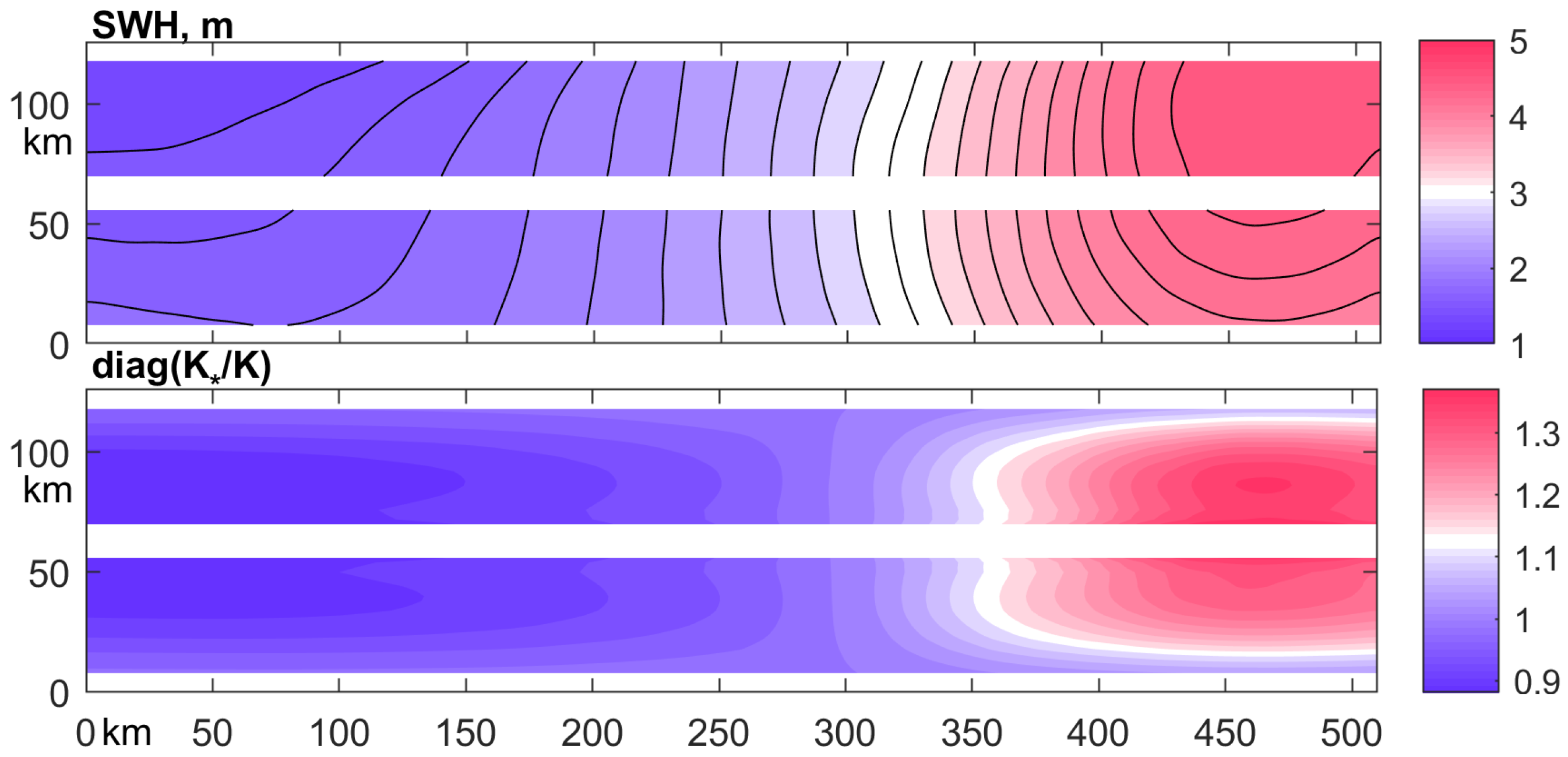
The diagonal elements of depend non-linearly on the distance of the SSH grid cell from nadir (i.e., across the swath) and on local SWH values, which can vary considerably along the swath (Figure 1, upper panel). However, the non-linearity of the SWH projection on the KaRIn noise error variance (Figure 5 of [8]) dumps spatial variations of in such a way that even a transition from calm (SWH∼1 m) conditions to stormy (SWH∼5 m) conditions along the swath (Figure 1) results only in a moderate (10–20%) deviation of from the block-diagonal pattern described by Equation (8) [28]. Furthermore, estimation of the BC deviation parameter from Equation (7),
yields a -variation range of 10– for typical oceanic conditions, indicating that Equation (9) may provide an accurate approximation for the precision matrix and its square root.

Figure 1.
An example of a SWH map at the SWOT swath (upper panel, in meters), and the map of the KaRIn noise ratio , where is the KaRIn noise variance distribution when the SWH shown in the upper panel is averaged along the swath, thus satisfying the block-circulant condition.
Inversion of the BC representation (9) of can be done efficiently [33] by inverting (in parallel) diagonal blocks and then applying the result to the Fourier image of the swath followed by the inverse Fourier transform.
Furthermore, multiplication of a vector by can be substantially simplified by exploiting the fact that are rank-one matrices whose range is spanned by the cross-track modes of the systematic error variation: . Introducing the notation and , the RHS of Equation (9) can be rewritten in the form
where are rescaled versions of the across-swath uncertainty mode matrix . As a consequence, blockwise inversions in can be executed in parallel using the Woodbury formula for inverting low-rank perturbations of the identity in the cross-swath direction:
Using representation (12), it is possible to factorize in order to normalize SSH innovations (see Appendix A):
where matrices have orthonormal columns, satisfying the relationships , and are 4 × 4 matrices containing the respective singular values.
Finally, we note that since both and its BC approximation are symmetric, symmetry is preserved for their inverses, and the number of independent blocks in the structure of and decreases from for a general BC matrix to the integer part of , thus reducing the computational cost of algorithms operating with BC approximations of the covariance and precision matrices.
3. Testing the BC Approximation
Evaluation of BC performance was done via the OSSE technique similar to the one used in [28] for assessment of the block-diagonal approximation: ensembles of 2D variational (2DVAR) DA experiments have been made by randomly perturbing “true” SSH distributions to simulate background states and observations with prescribed perturbation statistics. Misfits between the “true” background states and those retrieved from the DA runs as well as the computational cost of the retrievals with BC approximation were then compared with the retrievals obtained using a simplified (uncorrelated) and exact observational error statistics.
3.1. Ocean Simulation
To simulate the “true” ocean, we used a 4-month output of the Navy Coastal Ocean Model (NCOM [34]) east of Greenland. The model was run at 1 km resolution in June–September 2019 in the region of the East Greenland Current, nested within a coarser (4 km) configuration that was used to study the impact of freshwater runoff from the Greenland ice sheet on the local coastal circulation [35]. Apart from the runoff, the solution was forced by atmospheric fluxes of heat, freshwater, and momentum from the Navy Global Environmental Model (NAVGEM) [36]. To explore the dependence of BC approximation quality on the background current, three 128 km wide and 512 km long model snapshots with various RMS magnitudes (5, 7.5, and 10 cm) of the SSH variability were extracted from the NCOM simulation. More details on the model setting, including a regional map with model snapshots (an example is also given in Section 3.2), can be found in [28].
3.2. Simulation of Error Statistics
In the 2DVAR experiments, both modeling (background) and observation errors were represented by random realizations of the Gaussian 2D fields with zero mean and prescribed non-diagonal covariance matrices. The background error covariance was assumed to be isotropic, while the observation (SWOT) error covariance was anisotropic and defined by Equation (7).
3.2.1. Observation Errors
Recent releases of SWOT high-level ocean products [15] are the result of elimination of systematic errors contributing to the error budget of the observed SSH fields arising from various sources. Although the magnitude of these errors has been decimated by sophisticated data-driven calibration algorithms [7], the SWOT team also provides low-level (raw) products [19], which gives the community an opportunity to customize and improve the calibration of SSH observations [37,38].
Of particular importance are the errors driven by variations in the geometry and orientation of the on-board interferometer. These errors provide the major contribution to the error budget and can be as large as 1 m in magnitude at along-swath scales of thousands of kilometers [38]. Although their deterministic part is well-described by the STOP21 model, relatively small residuals (∼1 cm in magnitude) may still remain in the high-level products due to uncertainties in modeling transitions through the orbit eclipses and/or random components from the gyrometer [7]. Statistics of these residual errors are described by the second term in the RHS of (7) and mostly affect submesoscale oceanic variability at scales below 50 km.
To estimate the magnitude of the residual errors, we analyzed the high-frequency component of the SWOT data release [15] for the period between 1 April and 27 June 2023. These data were obtained during the 1-day repeat orbit, extracted at the calibration site west of California [12] and filtered using a high-pass Gaussian kernel with a half-width of 4 km (left panel in Figure 2). The respective across- and along-swath spectra (right panel in Figure 2) were normalized and averaged over the 88 daily snapshots. Figure 2 indicates the presence of these residual errors in the form of across-swath linear patterns of approximately 1–2 cm in magnitude causing the displacement of the along-swath spectral maximum toward higher frequencies.
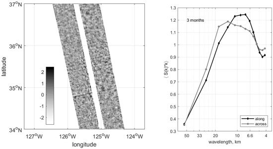
Figure 2.
Left: High-pass filtered SSH map (centimeters) obtained by SWOT on 16 May 2023 west of California. Right: Normalized by the total energy along- and across-swath spectra averaged in April–June 2023 over both halves of the swath segments shown in the left panel.
The obtained estimate of a systematic error magnitude of 1 cm roughly corresponds to the 1000 km long-wave cutoff of the along-swath error power spectra in Equation (7), suggesting that numerical experimentation with a 500 km long swath segment would be quite adequate for the purpose of simulating the residual error fields in testing the BC approximation.
3.2.2. Background Errors
The background fields simulating uncertain “model forecasts” were specified by imposing the background noise on the true solutions , extracted from the model run described in Section 3.1:
where is a realization of the 2D Gaussian random field with zero mean and unit variance, is a diagonal matrix of spatially homogeneous standard deviations from the true fields caused by the model (background) errors, and is the RMS variation of the true field. The coefficient controlling the magnitude of the background errors was varied in the course of the experiments. Similar to the SWOT observation errors, the model errors were assumed to be Gaussian, with a correlation matrix proportional to
where is the discretized Laplacian operator with Neumann boundary conditions at the swath edges, and a is the decorrelation scale, which was then also varied in the course of the experiments. The kernel (15) with km was also used to filter SWOT data in Figure 2.
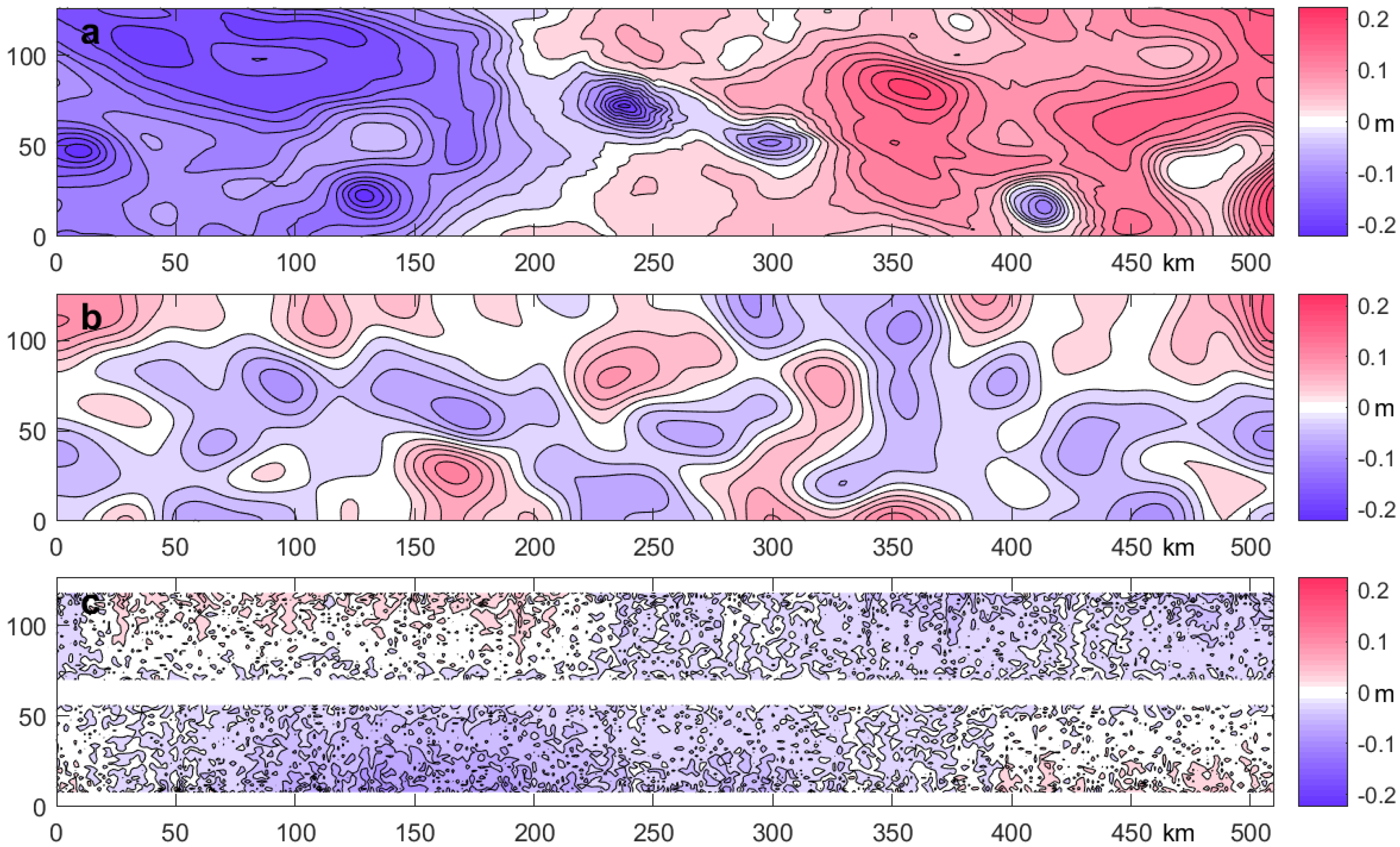
Similar to [28], the OSSEs were conducted on a rectangular 128 × 512 km grid at 2 km resolution (Figure 3). The “true” states used in [28] (an example is shown in Figure 3a) were interpolated on that grid to generate the ensemble of random realizations of the background error fields (Figure 3b) using Equation (14). Simulated SWOT error fields (Figure 3c) were collocated with the grid points of the background states.
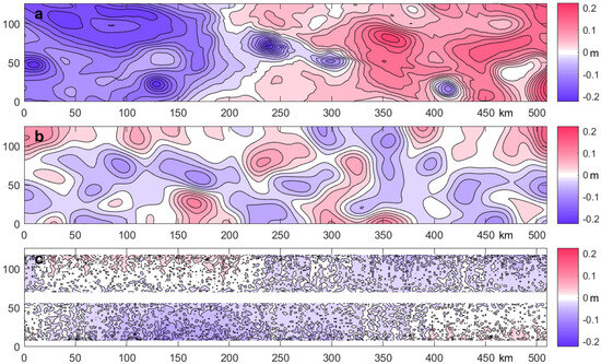
Figure 3.
(a) True SSH field (NCOM output on 20 July 2019) used in the assimilation experiments; (b) random realizations of the simulated background field; (c) SWOT observation error field.
3.3. Methodology of the OSSEs
The utility of the BC approximation was assessed by averaging the computation times and retrieval skills of the ensembles of 2DVAR DA runs performed with the exact SWOT error covariance model (7), using its block-circulant and diagonal approximations. Each ensemble had 100 members obtained by perturbing a single true state by random observations with zero mean and covariance as described in the previous section. Each ensemble was characterized by a fixed set of parameters, quantifying the statistics of the perturbations: the decorrelation scale (a = 4, 6, 10, 16) km and magnitude ( = 0.1, 0.2, 0.4, 0.8) of the background error covariance. The third parameter was the SWH magnitude, controlling the contribution of KaRIn noise to the SWOT error covariance in Equation (7). We used three realistic SWH patterns in the Greenland Sea corresponding to stormy conditions (spatially averaged SWH m), intermediate conditions ( m), and calm conditions ( m). The RMS spatial variation of SWH for these states, which defines the BC approximation accuracy, was, respectively, 1.1 m (upper panel in Figure 1), 0.3 m, and 0.1 m. The respective approximation errors of these SWH fields by their along-swath averages were 18%, 2%, and 0.6%.
Varying the parameters , and as mentioned above yields = 48 ensembles for each of the three true states. Since each 2DVAR DA experiment was run 3 times with exact, diagonal, and BC approximation of , the total number of the DA experiments was 48 × 9 = 432. Results of these experiments were assessed in two aspects: computational cost and the retrieval skill of the true states.
The retrieval skills were quantified using the error reduction ratios as follows:
Here, is the background error, angular brackets denote the ensemble averages, an overline denotes the standard deviation of a field in horizontal, while indices enumerate increments obtained using the exact (1) and diagonal (2) models of the SWOT error covariance, respectively. For the error reduction ratio with respect to the background state, the index j is set to zero, implying that the increment (i.e., the skill was assessed with respect to the background error, without assimilation). Figure 4 shows a background ensemble member obtained by contaminating the true state in Figure 3a with the background noise (Figure 3b) and the result of 2DVAR assimilation of simulated SWOT observations.
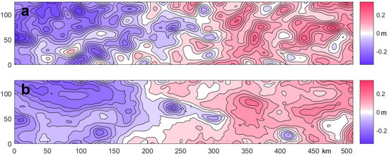
Figure 4.
(a) A random realization of the background field in Figure 3a with km and ; and (b) the result of its analysis using simulated SWOT observations with SWH m.
The computational cost was specified as the ensemble average of the CPU time required by the preconditioned conjugate gradient solver of in Equation (3). We considered two cases in representing : with and without the second term in Equation (7). The first case was solved with the diagonal preconditioner , whereas in the second case, the BC approximation of the SWOT precision matrix (Equation (12)) was used (Equation (5)).
A limited number of experiments have been done with the factorized version (4) of the analysis equation adopted by the operational system of the Naval Research Laboratory [22]. The computational efficiency e of the BC approximation was quantified by the ratio of the ensemble-averaged CPU times required for the analyses using the exact (Equation (7)) and diagonal ( in Equation (7)) representations of the SWOT error covariance:
In the 2DVAR runs with the exact representation of the SWOT error statistics, the BC preconditioner (12) was used.
4. Results
4.1. Retrieval Skill
Approximation (12) of the precision matrix provides an efficient preconditioner for solving Equation (5) with the spatially correlated model of the SWOT error covariance. In experiments comparing the retrieval skill (Equation (16)) of the exact and diagonal representations of the SWOT error covariance, the solutions to the preconditioned analysis Equation (5) were equivalent to solving
where the ensembles of innovations were specified by sampling the background states and observations from the Gaussian distributions defined by Equations (14) and (15) and the SWOT covariance model (7).
Since statistics of for the diagonal approximation of the SWOT error covariance were not consistent with the analysis of Equation (19), the retrieval skill in the diagonal case was significantly lower than in the case when the exact spatially correlated error covariance was used in the analysis equation (Figure 5).
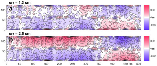
Figure 5.
Analysis error fields obtained for an ensemble member with the exact (a) and diagonal (b) representations of the observation error covariance matrices. The ensemble corresponds to the true state in Figure 3a, with the set of parameters characterized by the background error decorrelation scale km, noise level relative to the true state , and KaRIn noise error variance generated by surface waves under stormy conditions (SWH m). RMS values of both fields are shown.
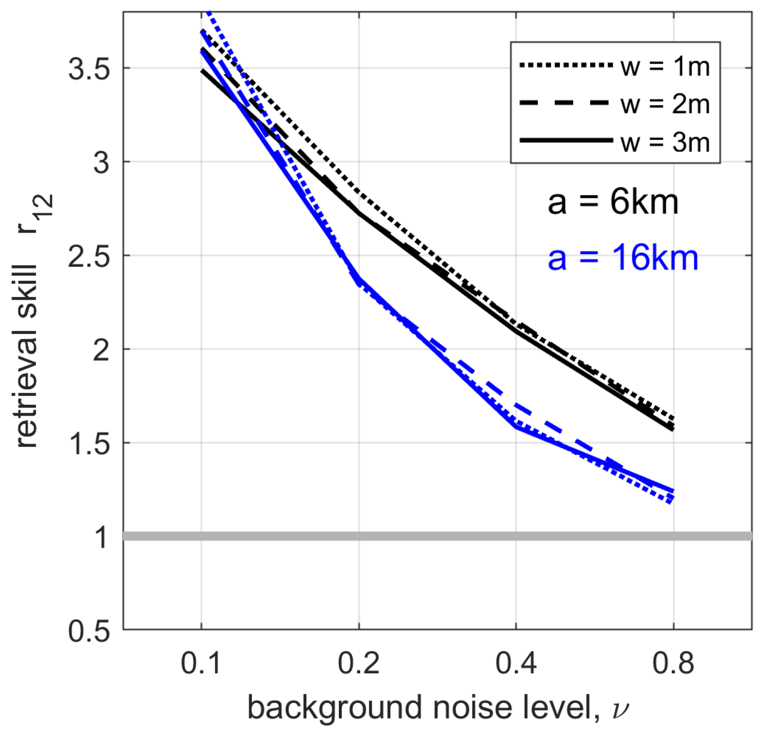
The advantage of using the spatially correlated error model was observed over the entire range of parameters characterizing statistics of the background and observation error fields. Results of these computations are summarized in Figure 6.
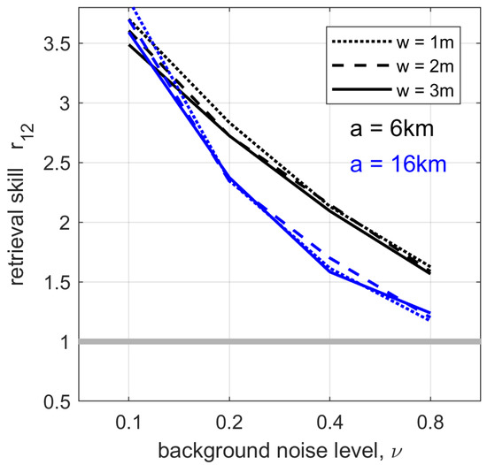
Figure 6.
Dependence of the retrieval skill (Equation (16)) on the background noise level and significant wave height w for two decorrelation scales.
It is interesting that the retrieval skill is insensitive to the SWH magnitude, which defines the relative contribution of the systematic error modes to the observation error statistics. This can be partly explained by the fact that these modes mostly contribute to the scales of variability exceeding 10 km that are efficiently penalized by the background term, which dominates the analysis error budget at . It is noteworthy that dependence on SWH becomes more significant at , when observation and background errors become comparable in magnitude. However, since the range of in most of the practical applications is 0.3–0.8, the impact of the SWH on the retrieval skill could be considered negligible.
Figure 6 also shows that using a spatially correlated error model becomes less advantageous with the increasing magnitude and decorrelation scale of the background SSH field. This conclusion can be explained by the growing dominance of the background error modes in the analysis equation. In the limiting case of very large background errors , the retrieval skill becomes indistinguishable from 1 at for km and for km.
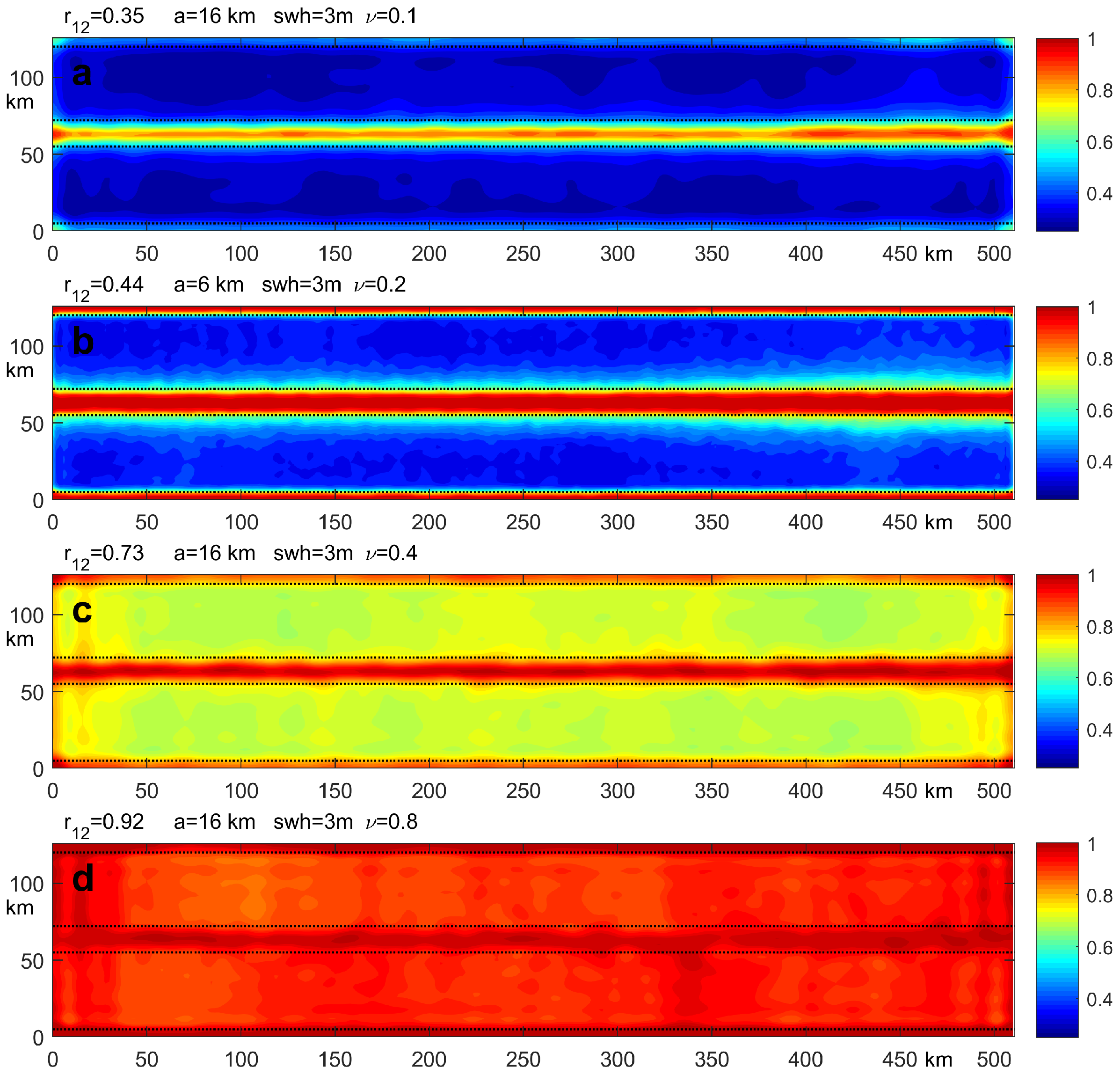
Spatial variation of the retrieval skill (Figure 7) further quantifies the utility of taking correlations of systematic errors into account. First, with the increasing decorrelation scale of background errors, information from relatively accurate SWOT SSH observations is able to leak into the nadir gap, unobservable by the KaRIn interferometer, thus providing a certain increase in skill in this area (cf. Figure 7a,b). At the same time, increase in the background error level widens the red area within the gap in Figure 7a,c,d, indicating that the advantage of taking the correlated errors into account is gradually lost as the uncertainty of the background field becomes the dominant factor in the 2DVAR analysis.
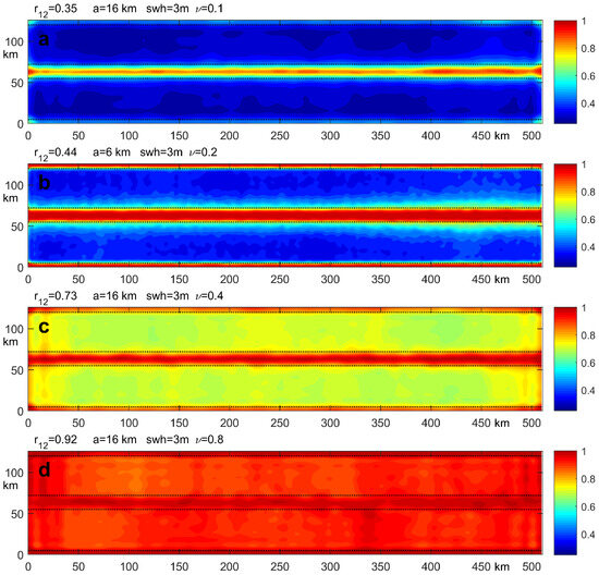
The patterns in Figure 7 also give a certain insight into the accuracy of the BC approximation. All the shown were obtained by averaging over the 2DVAR DA ensembles with the stormy SWH shown in Figure 1. In this case, the preconditioner matrix (Equation (5)) has the largest deviation from the exact one. Regarding this, it is necessary to note that, despite the minuscule value of for the SWH pattern in Figure 1, the respective approximation error of the preconditioning matrix
was 0.19, significantly reducing the convergence rate (Section 4.2). Nevertheless, it only slightly affected the retrieval skill, visible by its minuscule reduction in the right part of Figure 7a–c, which was caused by stronger inhomogeneity of the SWH field and, therefore, by larger BC approximation errors.
In summary, Figure 6 and Figure 7 demonstrate that the consideration of spatial correlations of the SWOT systematic residual errors in DA systems can be justified only when the background errors do not exceed 8–10 cm (). This upper limit on the magnitude of also depends on the decorrelation scale of the background errors and could be relaxed to some extent in regions dominated by submesoscale dynamics with km. In these regions, decays at a substantially slower rate (black lines in Figure 6). Further quantification of this threshold can be made if we consider the various aspects of the computational cost required for the computing the spatial correlations.
4.2. Computational Efficiency
In assessing the computational cost of solving the analysis in Equation (18), we compared the total CPU time required by the preconditioned conjugate gradient (PCG) solver with a diagonal preconditioner, , and a BC preconditioner, . Other solvers for symmetric positive definite systems were also tested but did not show any substantial difference with PCG.
The value of the quantification parameter e in Equation (17) is basically controlled by two factors: the CPU time T required by multiplication of a vector by , which grows quadratically with the decorrelation scale a, and the number of iterations n required for convergence, which grows roughly proportionally to the square root of the condition number of the preconditioned system matrix [23], §6.11.3 (using either or in Equation (12)). As a consequence,
where is the computational cost of the preconditioner relative to the cost of multiplication by the system matrix . In the explored range of background error parameters a and , the values of and changed in the ranges between (0.001–0.015) and (0.05–0.7), respectively, with the smaller values corresponding to the larger background decorrelation scale 16 km. The ratio of the number of iterations followed an opposite variation between 4.8 and 1.4, with the smaller values corresponding to larger values of a, , and w. In particular, dependence on w contributed to the increase in significantly for stormy conditions with m, when the BC approximation to had the largest error . In the typical ( m) and calm ( m) situations, the value of was much smaller (0.03 and 0.011, respectively) and did not affect the rate of convergence.
Figure 8 summarizes the results of these experiments. It is remarkable that, in contrast to the skill curves in Figure 6, the larger background scale has a visible advantage relative to the smaller one. This is due to the fact that, for km, becomes larger, while the numerator remains close to 1 due to the extremely low cost of the diagonal preconditioner. This significantly reduces the first fraction in the RHS of Equation (21), whereas the ratio of iteration numbers is not large enough to compensate for that reduction to the same extent as in the case of km. With the growth in the background noise, the black lines in Figure 8 dip below the threshold value of 1 at , making the BC preconditioner less computationally efficient than the diagonal one. However, it still keeps its superior skill in retrieving the true state at a significantly better (2 times) level (Figure 6). It is noteworthy that such situations (large background errors at small scales) are unlikely in the open ocean, because both modeling [39] and the latest SWOT observations [3] indicate that the SSH spectrum falls steeply with the wavenumber so that respective background errors should barely exceed 5 cm at scales below 5 km.
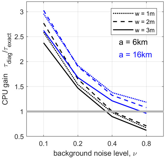
Figure 8.
Dependence of the computational cost parameter (Equation (17)) on the background noise level and significant wave height w for two decorrelation scales.
At larger scales (blue curves in Figure 8), the computational efficiency is better for the BC preconditioner up to the background noise level of 0.8, with the exception of stormy conditions at , where the solid blue line goes slightly below the threshold value. This favorable property is due to the relatively small magnitude of caused by the large cost of computing the action of the system matrix on a vector. Consequently, the first fraction in the RHS of Equation (21) becomes close enough to 1 to be compensated by 15–30% fewer iterations of the BC preconditioner at a large in the second fraction. For smaller background noise values, the advantage of the BC preconditioner at large scales was even more prominent (up to 5 times at ) due to the smaller contribution of to the system matrix.
Figure 8 also shows the minor role of sea surface roughness (controlled by SWH) in the computational efficiency of the BC preconditioners: for strongly inhomogeneous SWH distributions along the swath (typical for stormy conditions), the value of e degrades by approximately 10–20% over the entire range of the background noise levels. When the SWH spatial variability along the swath is relatively small (less than 10% of the mean value), the reduction in the computational efficiency is negligible, as it barely exceeds the confidence limits of averaging over the ensembles of experiments.
We also conducted a number of experiments with the renormalized version (4) of the analysis equation. This approach is implemented in the operational DA system of the Naval Research Laboratory for the case of uncorrelated observation errors [22]. The purpose of these experiments was to explore the possibility of extending the system to allow processing spatially correlated observations via a factorized version of the BC preconditioner (13). The retrieval skill was found to be almost identical to the one displayed in Figure 6; however, the computational efficiency was 10–15% worse, primarily because of the necessity to perform two multiplications (by and ) of a vector on every iteration.
5. Summary and Discussion
Arrival of early data from the SWOT mission has shown that the SSH variability observed by the satellite exceeds mission requirements in the submesoscale band at wavelengths below 25 km (Figure 1 in [3]). Special attention in SWOT calibration has focused on removing systematic errors caused by the uncertainties in the geometry and orientation of the on-board interferometer, which provides the largest contribution to the SWOT error budget [7]. Although the spatial structure of these error fields can be accurately described by STOP21 software and error covariance models developed by JPL, high-frequency along-swath components may still be present at the centimeter level in the calibrated products. It is therefore useful to investigate the utility of employing a spatially correlated model [14] in operational data assimilation algorithms that had been developed previously under the assumption of spatially uncorrelated observations.
In this study, we exploited the near-block-circulant structure of the SWOT covariance model and investigated the retrieval skill of the BC approximation to the SWOT precision matrix using simulated SSH patterns the East Greenland Sea at 1 km resolution. In contrast to the previous study [28] that had focused on the performance of the block-diagonal approximation of the SWOT precision matrix (which is mostly valid at the submesoscale), the BC approximation introduced here provides significantly better accuracy over a wider range of scales, limited from above only by the length of the analyzed swath segment. The retrieval skill of the BC approximation was assessed through the ensembles of 2DVAR assimilation experiments with variable error statistics of simulated SWOT observations and background states.
Results of the study are summarized as follows. The correlated SWOT errors significantly affect the analysis if the background noise does not exceed the magnitude of the background state for a wide range of sea surface roughness values. Similar to the block-diagonal approximation, the BC approximation is more efficient for typical (SWH∼1–2 m) surface roughness with moderate (10–20%) SWH variation along the swath. In contrast to BD, the BC approximation is weakly sensitive to SWH variation and remains valid under stormy conditions (Figure 1), providing better analysis as compared to an uncorrelated error model even at large background noise levels. This favorable feature of the BC approximation emerges because it is more general. The BD approximation is scale-selective and mostly valid for retrieving submesoscale features of SSH variability characterized by the flat error spectra at wavelengths below 50 km. The BC approximation, being free from this constraint, is also less sensitive to errors introduced by the spatial variations in the magnitude surface waves. In that respect, using the BC approximation of the precision matrix as a preconditioner persistently yields assimilation accuracy identical to the accuracy delivered by the exact JPL error covariance model with a diagonal preconditioner. This accuracy is, however, achieved at significantly (1.3–3 times, Figure 8) lower computational cost than what is observed with a diagonal preconditioner.
The BC approximation can be developed further to include environmental contributions in Equation (6). This could be accomplished by exploiting the block-circulant structure of the 2D Fourier transform in conjunction with separable types of the error spectra , such as isotropic power spectra , often used in large-scale atmospheric modeling.
The proposed approach can be instrumental for SSH products based entirely on satellite observations. In such applications, a (low-resolution) background state in the cost function could be derived from an image provided by traditional nadir altimeter(s) and then synthesized with higher resolution SWOT data using the described variational approach.
Evidently, the analysis presented here is based on OSSEs with idealized error statistics, employing Gaussian fields with covariances that are diagonalizable by the discrete Fourier transform. The ultimate test will be the forecast skill assessment of an operational system upgraded to handle spatially correlated SSH errors at 1 km resolution. This is the subject of our forthcoming research.
Author Contributions
Conceptualization, software, methodology, writing—original draft preparation: M.Y.; methodology, software, editing: C.B.; software, formal analysis: G.P., data acquisition, editing: J.D. All authors have read and agreed to the published version of the manuscript.
Funding
This research was funded by the ONR project number 73-6C95025 “Precision Assessment of Remotely Sensed data with Error Correlations” (PARSEC). C.B. was supported by NSF Grant DMS-1923221 and the ONR Summer Faculty Fellowship Program.
Data Availability Statement
The SWOT calibration altimetry data were downloaded from [15]. The NCOM simulation in the Greenland Sea used in this study are stored at the Navy DSRC server and can be obtained after obtaining an account at the facility in accordance with NRL policies. The corresponding author can be contacted for information to access the archived data once an account has been established.
Acknowledgments
The authors are grateful to B. Tchonang for providing SWOT observations in the Cal/Val region west of California and to S. Smith for the output of the NCOM model solutions in the East Greenland Sea.
Conflicts of Interest
The authors declare no conflicts of interest.
Appendix A. Factorization of the BC Approximation of the Precision Matrix
Assume that diagonal blocks in Equation (11) have the form
This would allow the factorization
Rearranging the RHS of Equation (A1) yields , so, without loss of generality, we can assume that for some that satisfies
This condition is consistent with (and, hence, ) being diagonal, although non-diagonal solutions are possible as well. Taking and choosing positive roots of (cf. Equation (A3)), we obtain
to arrive at a factorization of with
References
- Durand, D.; Fu, M.; Lettenemaier, L.L.; Alsdorf, D.; Rodriguers, E.; Esteban-Fernandez, D. The surface water and ocean topography mission: Observing terrestrial surface water and oceanic submesoscale eddies. Proc. IEEE 2010, 98, 766–779. [Google Scholar] [CrossRef]
- Esteban-Fernandez, D. SWOT Project: Mission Performance and Error Budget. Revision A, NASA. /JPL Tech. Rep. JPL D-79084. 2013; 83p. Available online: http://swot.jpl.nasa.gov/files/SWOT_D-79084_v5h6_SDT.pdf (accessed on 10 April 2024).
- Fu, L.L.; Pavelsky, T.; Cretaux, J.F.; Morrow, R.; Farrar, J.T.; Vaze, P.; Sengenes, P.; Vinogradova-Shiffer, N.; Sylvestre-Baron, A.; Picot, N.; et al. The surface water and ocean topography mission: A breakthrough in radar remote sensing of the ocean and land surface water. Geophys. Res. Lett. 2023, 51, e2023GL107652. [Google Scholar] [CrossRef]
- Ito, N.; Uematsu, A.; Yajima, Y.; Isoguchi, O. A Japanese new altimetry mission COMPIRA—Towards high temporal and spatial sampling of sea surface height. Agu Fall Meet. Abstr. 2014, 2014, OS34B-05. [Google Scholar]
- Chen, G.; Tnag, J.; Zhao, C.; Wo, S.; Yu, F.; Ma, C.; Xu, Y.; Chen, W.; Zhnag, Y.; Wi, L. Concept design of the Guanlan science mission: China’s novel contribution to space oceanography. Front. Mar. Sci. 2019, 6, 194. [Google Scholar] [CrossRef]
- SWOT Project: Product Description, Algorithm Theoretical Basis and Data, Level 2 KaRIn Low Rate Sea Surface Height Data Product, Version 1.1, 2023. Available online: https://podaac.jpl.nasa.gov/dataset/SWOT_L2_LR_SSH_1.1 (accessed on 26 May 2024).
- Dibarboure, G.; Ubelmann, C.; Flamant, B.; Briol, F.; Peral, E.; Bracher, G.; Vergara, O.; Faugère, Y.; Soulat, F.; Picot, N. Data-driven calibration algorithm and pre-launch performance simulations for the SWOT mission. Remote Sens. 2022, 14, 6070. [Google Scholar] [CrossRef]
- Gaultier, L.; Ubelmann, C.; Fu, L.-L. SWOT Simulator Documentation; Tech. Rep. 2.3.0, Jet Propulsion Laboratory; CalTech: Pasadena, CA, USA, 2017. [Google Scholar]
- Gaultier, L.; Ubelmann, C.; Fu, L.-L. The challenge of using future SWOT data for oceanic field reconstruction. J. Atm. Oceanic Tech. 2016, 33, 119–126. [Google Scholar] [CrossRef]
- Ma, C.; Guo, X.; Zhang, H.; Di, J.; Chen, G. An investigation of the influences of SWOT sampling and errors on ocean eddy observation. Remote Sens. 2020, 12, 2682. [Google Scholar] [CrossRef]
- Li, Z.; Wang, J.; Fu, L.-L. An observing system simulation experiment for ocean state estimation to assess the performance of the SWOT mission: Part 1—A twin experiment. J. Geophys. Res. Oceans 2019, 124, 4838–4855. [Google Scholar] [CrossRef]
- Wang, J.; Fu, L.-L.; Qui, B.; Menemenlis, D.; Farrar, J.T.; Chao, Y.; Thompson, A.F.; Flexas, M.M. An observing system simulation experiment for the calibration and validation of the SWOT sea surface height measurement using in situ platforms. J. Ocean Atm. Tech. 2018, 35, 281–297. [Google Scholar] [CrossRef]
- King, R.R.; Martin, M.J. Assimilating realistically simulated wide-swath altimeter observations in a high-resolution shelf-seas forecasting system. Ocean Sci. 2021, 17, 1701–1813. [Google Scholar] [CrossRef]
- Gaultier, L.; Ubelmann, C. SWOT Science Ocean Simulator Open Source Repository. 2022. Available online: https://github.com/SWOTsimulator/swotsimulator (accessed on 13 March 2024).
- SWOT Project: Release Note KaRIn Science Data Products, Version C. 2024. Available online: https://podaac.jpl.nasa.gov/dataset/SWOT_L2_LR_SSH_2.0 (accessed on 26 May 2024).
- Ubelmann, C.; Dibarboure, G.; Dubois, P. A cross-spectral approach to measure the error budget of the SWOT altimetry mission over the ocean. J. Ocean Atm. Tech. 2018, 35, 845–857. [Google Scholar] [CrossRef]
- Beauchamp, M.; Febvre, Q.; Georgenthum, H.; Fablet, R. 4DVarNet-SSH: End-to-end learning of variational interpolation schemes for nadir and wide-swath satellite altimetry. Geosci. Model Dev. 2023, 16, 2119–2147. [Google Scholar] [CrossRef]
- Tréboutte, A.; Carli, E.; Ballarotta, M.; Carpentier, B.; Faugère, Y.; Dibarboure, G. KaRIn noise reduction using a convolutional neural network for the SWOT ocean products. Remote Sens. 2023, 15, 2183. [Google Scholar] [CrossRef]
- SWOT Project: Release Note KaRIn Science Data Products, Version C. 2024. Available online: https://podaac.jpl.nasa.gov/dataset/SWOT_L2_LR_SSH_EXPERT_2.0 (accessed on 26 May 2024).
- Rosmond, T.; Xu, L. Development of NAVDAS-AR: Non-linear formulation and outer loop nests. Tellus 2006, 58A, 45–58. [Google Scholar] [CrossRef]
- Fletcher, S.J. Observation space variational data assimilation methods. In Data Assimilation Methods for the Geosciences; Elsevier: Amsterdam, The Netherlands, 2022; pp. 785–795. [Google Scholar] [CrossRef]
- Cummings, J.A.; Smedstad, O.M. Variational data analysis for the global ocean. In Data Assimilation for Atmospheric, Oceanic and Hydrologic Applications Vol. II; Park, S.K., Xu, L., Eds.; Springer: Berlin/Heidelberg, Germany, 2013. [Google Scholar]
- Saad, Y. Iterative Methods for Sparse Linear Systems; SIAM Press: Philadelphia, PA, USA, 2003; 547p, Available online: https://epubs.siam.org/doi/book/10.1137/1.9780898718003 (accessed on 26 May 2024).
- Ruggiero, G.A.; Cosme, E.; Brankart, J.M.; Le Sommer, J.; Ubelmann, C. An efficient way to account for observation error correlations in the assimilation of data from the future SWOT high-resolution altimeter mission. J. Ocean Atm. Tech. 2016, 33, 2755–2768. [Google Scholar] [CrossRef]
- Yaremchuk, M.; D’Addezio, J.; Jacobs, G. Facilitating inversion of the error covariance models for the wide-swath altimeters. Remote Sens. 2020, 12, 1823. [Google Scholar] [CrossRef]
- Metref, S.; Cosme, E.; Guillou, F.L.; Sommer, J.L.; Brankart, J.-M.; Verron, J. Wide-swath altimetric satellite data assimilation with correlated error reduction. Front. Mar. Sci. 2020, 6, 822. [Google Scholar] [CrossRef]
- Yaremchuk, M. Sparse approximation of the precision matrices for the wide-swath altimeters. Remote Sens. 2022, 14, 2827. [Google Scholar] [CrossRef]
- Yaremchuk, M.; Beattie, C.; Panteleev, G.; d’Addezio, J.; Smith, S. The effect of spatially correlated errors on sea surface height retrieval from SWOT altimetry. Remote Sens. 2023, 15, 4277. [Google Scholar] [CrossRef]
- Ubelmann, C.; Fu, L.-L.; Brown, S.; Peral, E.; Esteban-Fernandez, D. The effect of atmospheric water vapor content on the performance of future wide-swath ocean altimetry measurement. J. Atmos. Ocean Technol. 2014, 31, 1446–1454. [Google Scholar] [CrossRef]
- Gao, Z.; Chen, G.; Ma, C.; Zhao, C.; Zhang, B. The effect of differential tropospheric error on the measurement of wide-swath interferometric altimetry. IEEE Trans. Geosci. Remote Sens. 2023, 61, 5222011. [Google Scholar] [CrossRef]
- Li, Z.; McWiliams, J.C.; Ide, K.; Farrara, J.D. A multi-scale variational data assimilation scheme: Formulation and illustration. Mon. Wea. Rev. 2015, 143, 3804–3822. [Google Scholar] [CrossRef]
- de Moraes, R.J.; Hajibeygi, H.; Jansen, J.D. A multiscale method for data assimilation. Comput. Geosci. 2020, 24, 425–442. [Google Scholar] [CrossRef]
- De Mazancourt, T.; Gerlic, D. The inverse of a block-circulant matrix. IEEE Trans. Antennas Propag. 1983, 31, 808–810. [Google Scholar] [CrossRef]
- Barron, C.N.; Kara, A.B.; Martin, P.J.; Rhodes, R.C.; Smedstad, L.F. 2006: Formulation, implementation and examination of vertical coordinate choices in the Global Navy Coastal Ocean Model (NCOM). Ocean. Model. 2006, 11, 347–375. [Google Scholar] [CrossRef]
- Helber, R.W.; Smith, S.R.; Panteleev, G.; Shriver, J.; Pickard, R. Greenland Freshwater Stability in the East Greenland Current. Deep Sea Res. 2023; in press. [Google Scholar]
- Hogan, T.F.; Liu, M.; Ridout, J.A.; Peng, M.S.; Whitcomb, T.R.; Ruston, B.C.; Reynolds, C.A.; Eckermann, S.D.; Moskaitis, J.R.; Baker, N.L.; et al. The Navy Global Environmental Model. Oceanography 2014, 27, 116–125. [Google Scholar] [CrossRef]
- Jacobs, G.; Barron, C.; Fox, D.N.; Whitmer, K.R.; Klingenberger, S.; May, D.; PBlaha, J.P. Operational altimeter sea level products. Oceanography 2002, 15, 13–21. [Google Scholar] [CrossRef]
- Jacobs, G.; Desai, S.; D’Addezio, J.; Bartels, B. SWOT cross-track error characteristics estimated from observations. Geophys. Res. Lett. 2024; under review. [Google Scholar]
- Souopgui, I.; D’Addezio, J.; Rowley, C.D.; Smith, S.R.; Jacobs, G.A.; Helber, R.W.; Yaremchuk, M.; Osborne, J. Multi-scale assimilation of simulated SWOT observations. Ocean. Model. 2020, 154, 101683. [Google Scholar] [CrossRef]
Disclaimer/Publisher’s Note: The statements, opinions and data contained in all publications are solely those of the individual author(s) and contributor(s) and not of MDPI and/or the editor(s). MDPI and/or the editor(s) disclaim responsibility for any injury to people or property resulting from any ideas, methods, instructions or products referred to in the content. |
© 2024 by the authors. Licensee MDPI, Basel, Switzerland. This article is an open access article distributed under the terms and conditions of the Creative Commons Attribution (CC BY) license (https://creativecommons.org/licenses/by/4.0/).

