
Zero-Shot SAR Target Recognition Based on a Conditional Generative Network with Category Features from Simulated Images


Abstract
1. Introduction
- The category features constructed from the simulated images are proposed. The feasibility of these category features utilized as the category auxiliary information for SAR zero-shot learning is verified.
- A framework for zero-shot generation of SAR data based on the conditional VAE-GAN is proposed. The network establishes a connection between the seen and the unseen class data through the category features. By learning the mapping from the category features to the real data using the seen class data, it can generate the unseen class data.
- Compared to the embedding model-based methods assisted by the semantic information, our architecture can recognize multiple unseen class SAR targets instead of inferring a single one.
2. Methodology
2.1. Symbolic Representation of Zero-Shot Target Recognition
2.2. The Feature Extraction Module
2.2.1. Extraction of the Real Features
2.2.2. Extraction of Category Features
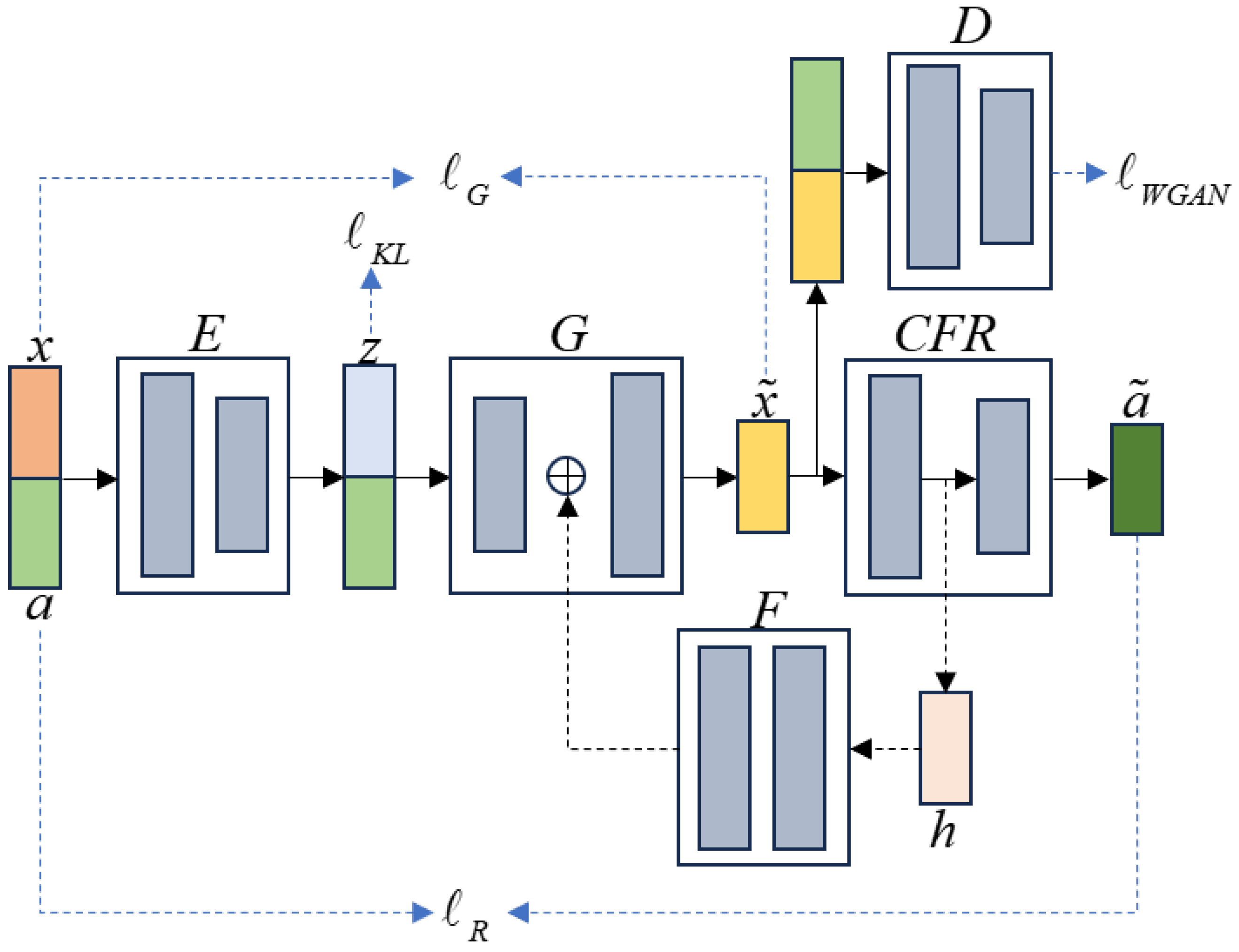
2.3. The Feature Generation Module
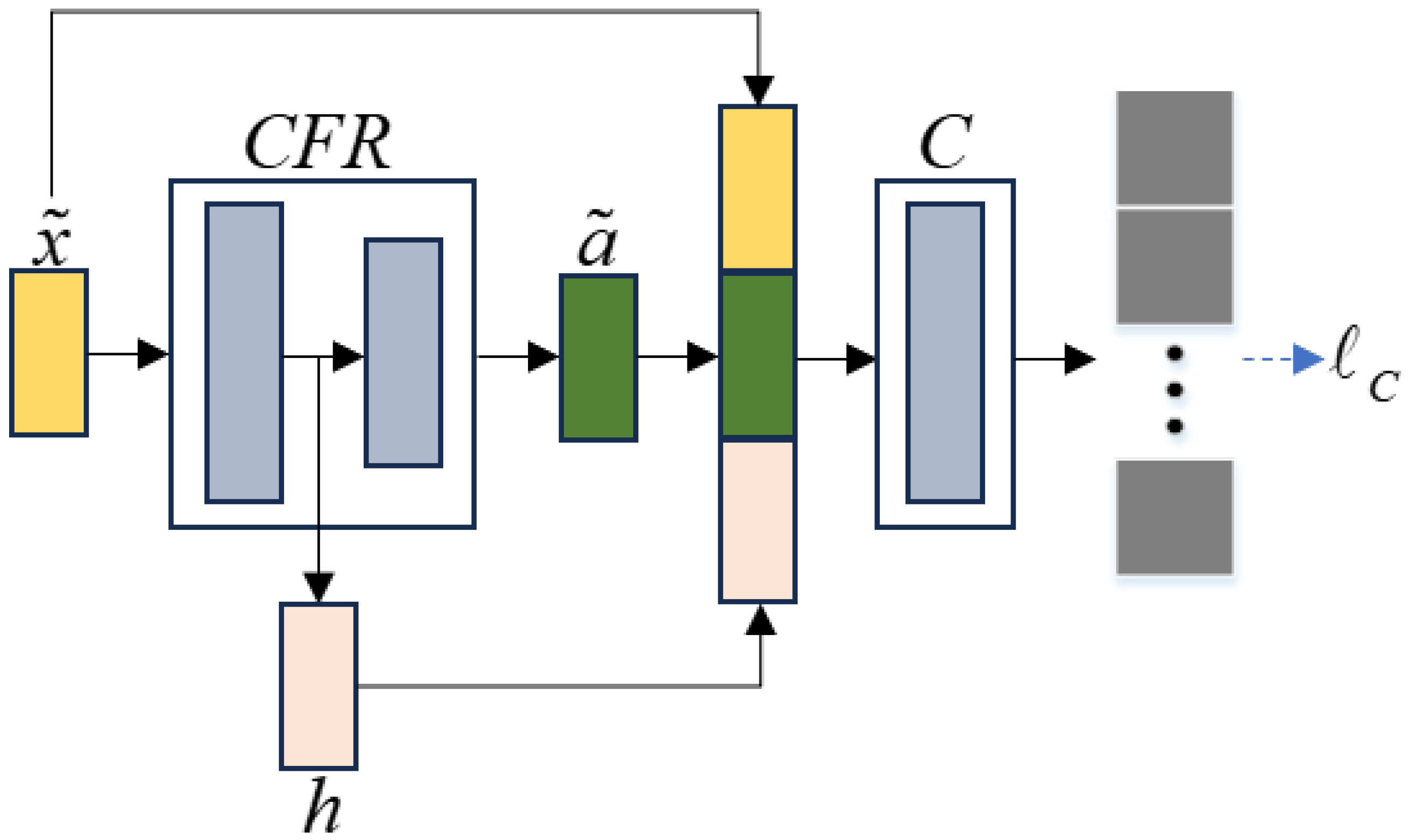
2.4. The Classification Module
2.5. Training and Test Process
3. Experiments
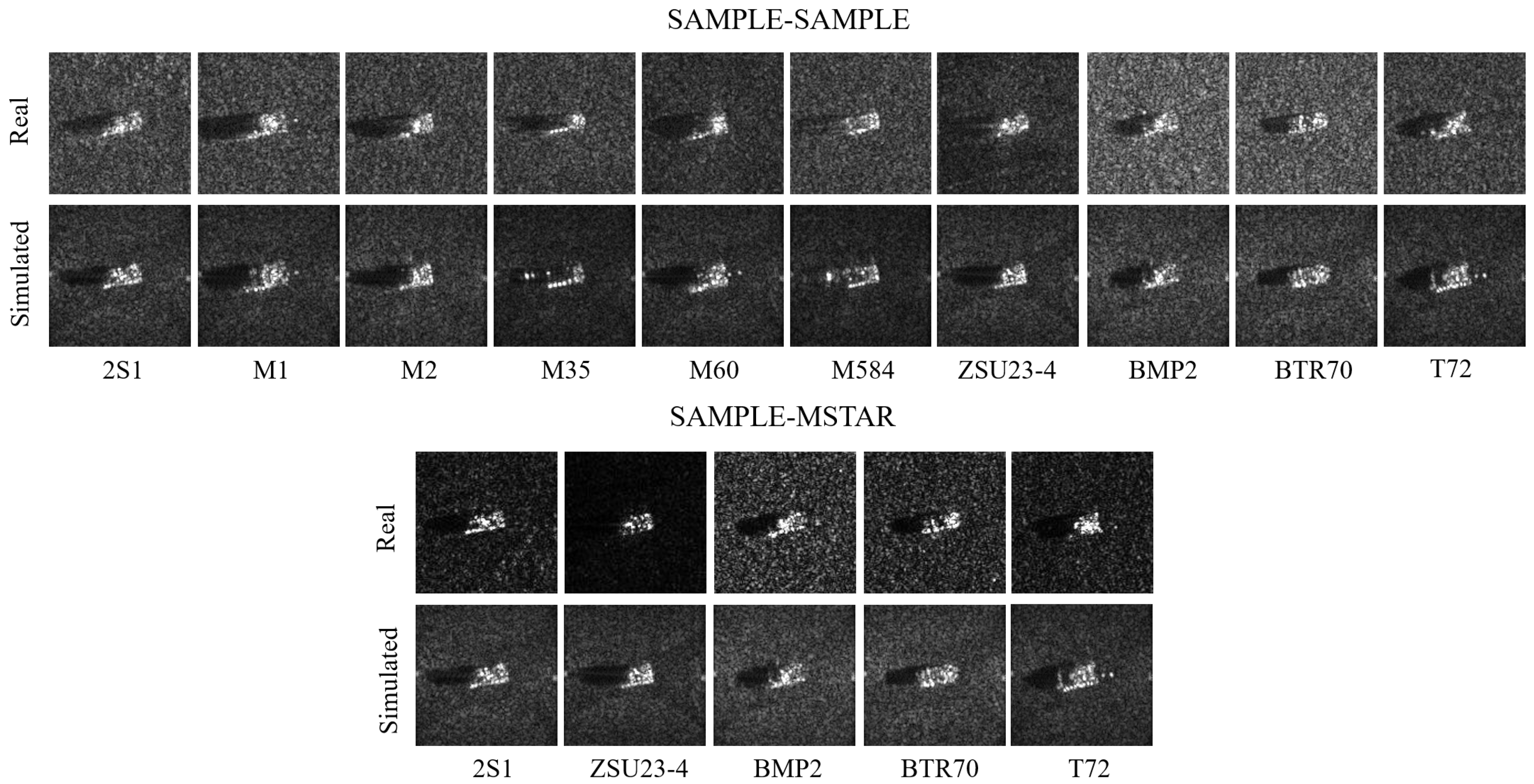
3.1. Datasets
3.2. Effectiveness of the Method
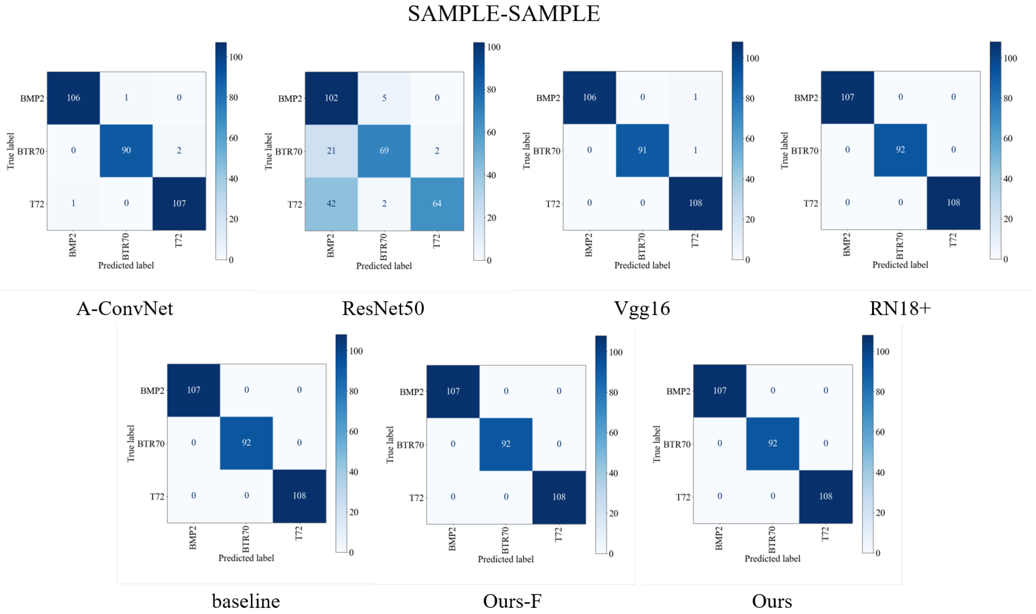
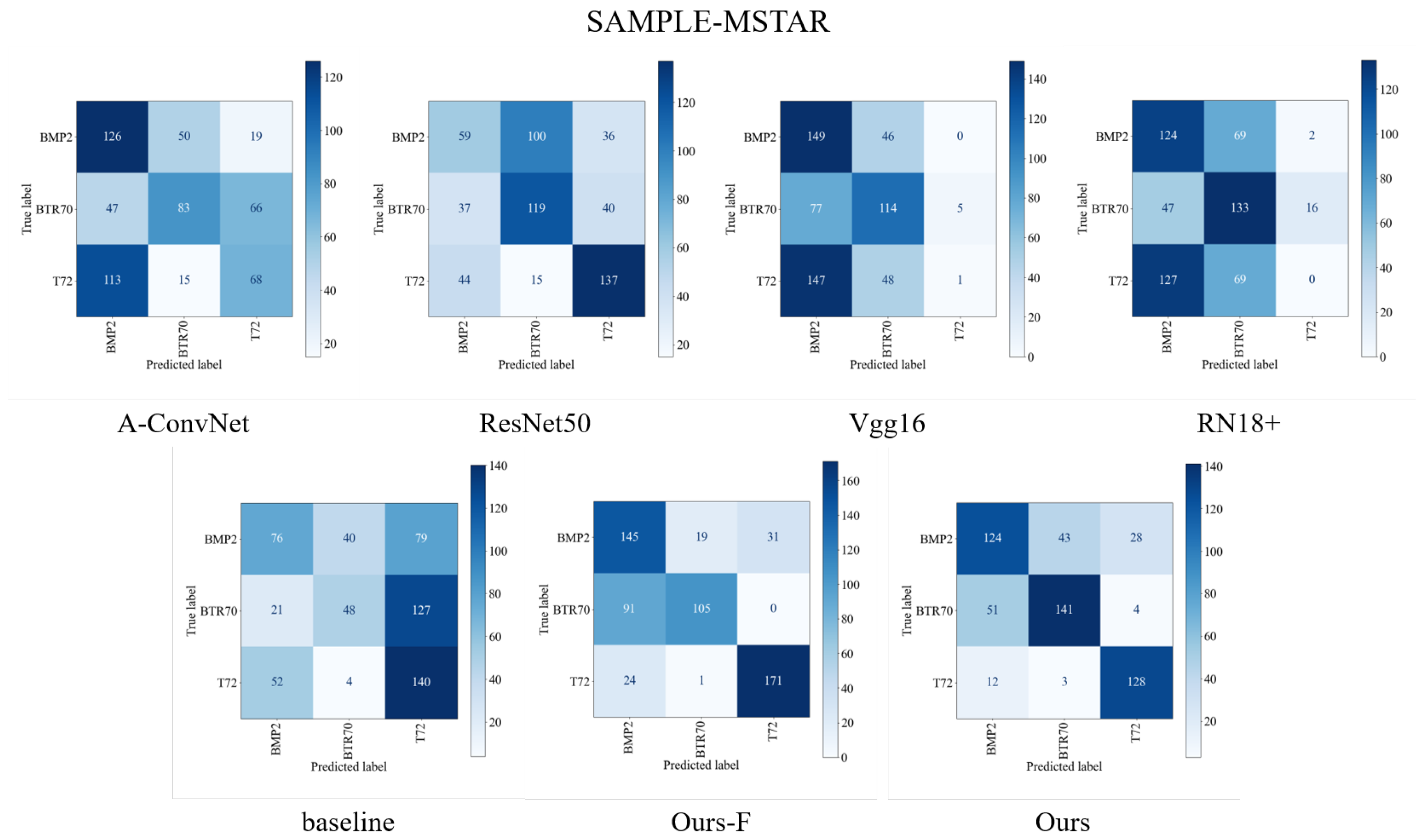
3.2.1. The Analysis of the Experimental Results
3.2.2. The Significance Test of the Experimental Results
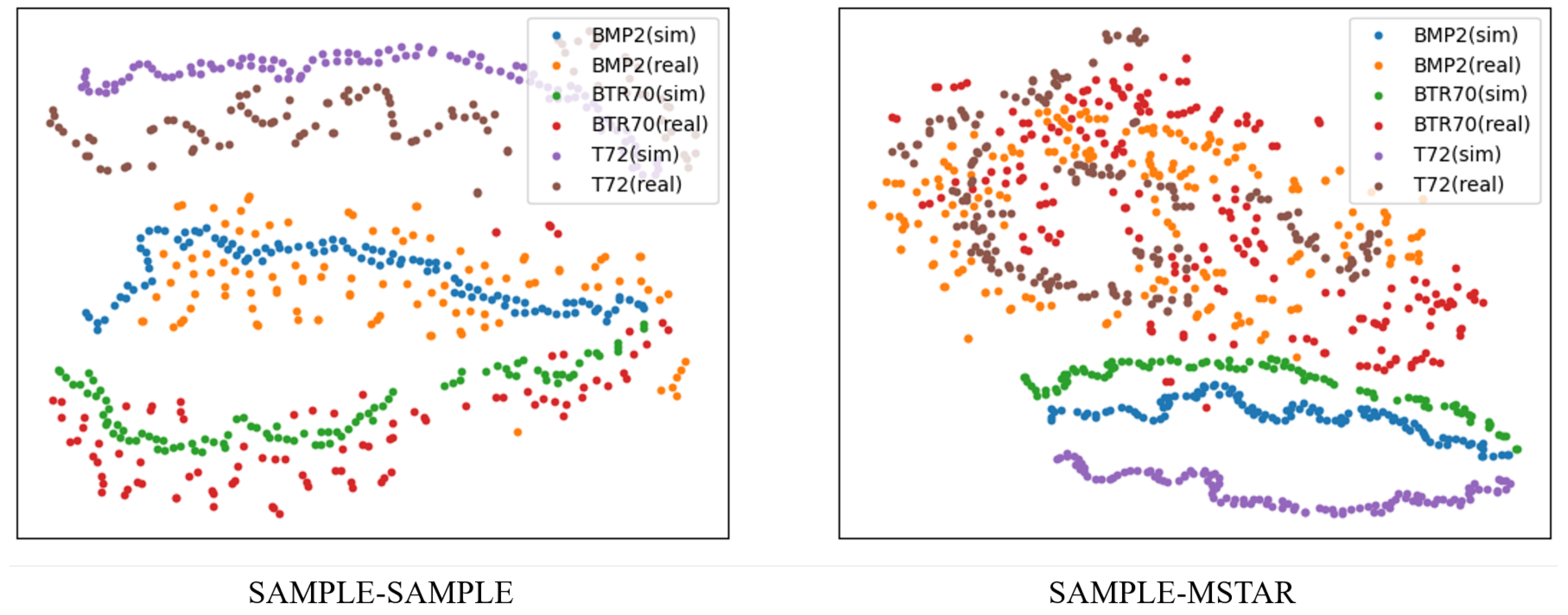
3.2.3. The Analysis of the Differences between the Two Experimental Groups
3.3. Impact of the Intermediate Layer Dimension Size
3.4. Impact of the Number of Simulated and Real Images
3.5. Impact of the Seen Class Number
3.6. Extended Experiments on the Generalized Zero-Shot Recognition
4. Discussion
- The deep features utilized for network learning in this paper are extracted solely from a model pre-trained on seen class real images. It may limit their representational capacity thereby influencing the learning of the network.
- The proposed method relies on the similarity of the features between the seen and the unseen class targets, allowing for the transfer of the mapping learned from the seen classes to the unseen classes. If there is a significant difference between the seen and the unseen classes, the proposed method may have limitations.
5. Conclusions
Author Contributions
Funding
Data Availability Statement
Acknowledgments
Conflicts of Interest
References
- Khoshnevis, S.A.; Ghorshi, S. A tutorial on tomographic synthetic aperture radar methods. SN Appl. Sci. 2020, 2, 1504. [Google Scholar] [CrossRef]
- Dudgeon, D.E.; Lacoss, R.T. An overview of automatic target recognition. Linc. Lab. J. 1993, 6, 3–10. [Google Scholar]
- Popova, M.; Shvets, M.; Oliva, J.; Isayev, O. MolecularRNN: Generating realistic molecular graphs with optimized properties. arXiv 2019, arXiv:1905.13372. [Google Scholar]
- Shaulskiy, D.V.; Evtikhiev, N.N.; Starikov, R.S.; Starikov, S.N.; Zlokazov, E.Y. MINACE filter: Variants of realization in 4-f correlator. In Proceedings of the Optical Pattern Recognition XXV, Baltimore, MD, USA, 5–9 May 2014; SPIE: Bellingham, WA, USA, 2014; Volume 9094, pp. 135–142. [Google Scholar]
- Diemunsch, J.R.; Wissinger, J. Moving and stationary target acquisition and recognition (MSTAR) model-based automatic target recognition: Search technology for a robust ATR. In Proceedings of the Algorithms for Synthetic Aperture Radar Imagery V, Orlando, FL, USA, 13–17 April 1998; SPIE: Bellingham, WA, USA, 1998; Volume 3370, pp. 481–492. [Google Scholar]
- Li, J.; Yu, Z.; Yu, L.; Cheng, P.; Chen, J.; Chi, C. A Comprehensive Survey on SAR ATR in Deep-Learning Era. Remote Sens. 2023, 15, 1454. [Google Scholar] [CrossRef]
- Krizhevsky, A.; Sutskever, I.; Hinton, G.E. Imagenet classification with deep convolutional neural networks. Adv. Neural Inf. Process. Syst. 2012, 25, 1–9. [Google Scholar] [CrossRef]
- Simonyan, K.; Zisserman, A. Very deep convolutional networks for large-scale image recognition. arXiv 2014, arXiv:1409.1556. [Google Scholar]
- He, K.; Zhang, X.; Ren, S.; Sun, J. Deep residual learning for image recognition. In Proceedings of the IEEE Conference on Computer Vision and Pattern Recognition, Las Vegas, NV, USA, 27–30 June 2016; pp. 770–778. [Google Scholar]
- Pearlmutter. Learning state space trajectories in recurrent neural networks. In Proceedings of the International 1989 Joint Conference on Neural Networks, Washington, DC, USA, 18–22 June 1989; IEEE: Piscataway, NJ, USA, 1989; pp. 365–372. [Google Scholar]
- Scarselli, F.; Tsoi, A.C.; Gori, M.; Hagenbuchner, M. Graphical-based learning environments for pattern recognition. In Proceedings of the Structural, Syntactic, and Statistical Pattern Recognition: Joint IAPR International Workshops, SSPR 2004 and SPR 2004, Lisbon, Portugal, 18–20 August 2004; Proceedings. Springer: Berlin/Heidelberg, Germany, 2004; pp. 42–56. [Google Scholar]
- Morgan, D.A. Deep convolutional neural networks for ATR from SAR imagery. In Proceedings of the Algorithms for Synthetic Aperture Radar Imagery XXII, Baltimore, MD, USA, 20–24 April 2015; SPIE: Bellingham, WA, USA, 2015; Volume 9475, pp. 116–128. [Google Scholar]
- Chen, S.; Wang, H.; Xu, F.; Jin, Y.Q. Target classification using the deep convolutional networks for SAR images. IEEE Trans. Geosci. Remote Sens. 2016, 54, 4806–4817. [Google Scholar] [CrossRef]
- Zhang, F.; Hu, C.; Yin, Q.; Li, W.; Li, H.C.; Hong, W. Multi-aspect-aware bidirectional LSTM networks for synthetic aperture radar target recognition. IEEE Access 2017, 5, 26880–26891. [Google Scholar] [CrossRef]
- Zhao, C.; Zhang, S.; Luo, R.; Feng, S.; Kuang, G. Scattering features spatial-structural association network for aircraft recognition in SAR images. IEEE Geosci. Remote. Sens. Lett. 2023, 20, 4006505. [Google Scholar] [CrossRef]
- Zhang, X.; Feng, S.; Zhao, C.; Sun, Z.; Zhang, S.; Ji, K. MGSFA-Net: Multi-Scale Global Scattering Feature Association Network for SAR Ship Target Recognition. IEEE J. Sel. Top. Appl. Earth Obs. Remote. Sens. 2024, 17, 4611–4625. [Google Scholar] [CrossRef]
- Ding, J.; Chen, B.; Liu, H.; Huang, M. Convolutional neural network with data augmentation for SAR target recognition. IEEE Geosci. Remote Sens. Lett. 2016, 13, 364–368. [Google Scholar] [CrossRef]
- Ding, B.; Wen, G.; Huang, X.; Ma, C.; Yang, X. Data augmentation by multilevel reconstruction using attributed scattering center for SAR target recognition. IEEE Geosci. Remote Sens. Lett. 2017, 14, 979–983. [Google Scholar] [CrossRef]
- Guo, J.; Lei, B.; Ding, C.; Zhang, Y. Synthetic aperture radar image synthesis by using generative adversarial nets. IEEE Geosci. Remote Sens. Lett. 2017, 14, 1111–1115. [Google Scholar] [CrossRef]
- Cui, Z.; Zhang, M.; Cao, Z.; Cao, C. Image data augmentation for SAR sensor via generative adversarial nets. IEEE Access 2019, 7, 42255–42268. [Google Scholar] [CrossRef]
- Niu, S.; Qiu, X.; Peng, L.; Lei, B. Parameter prediction method of SAR target simulation based on convolutional neural networks. In Proceedings of the EUSAR 2018; 12th European Conference on Synthetic Aperture Radar, Aachen, Germany, 4–7 June 2018; VDE: Frankfurt am Main, Germany, 2018; pp. 1–5. [Google Scholar]
- Zhai, Y.; Deng, W.; Xu, Y.; Ke, Q.; Gan, J.; Sun, B.; Zeng, J.; Piuri, V. Robust SAR automatic target recognition based on transferred MS-CNN with L 2-regularization. Comput. Intell. Neurosci. 2019, 2019, 9140167. [Google Scholar] [CrossRef] [PubMed]
- Malmgren-Hansen, D.; Kusk, A.; Dall, J.; Nielsen, A.A.; Engholm, R.; Skriver, H. Improving SAR automatic target recognition models with transfer learning from simulated data. IEEE Geosci. Remote Sens. Lett. 2017, 14, 1484–1488. [Google Scholar] [CrossRef]
- Zelong, W.; Xianghui, X.; Lei, Z. Study of deep transfer learning for SAR ATR based on simulated SAR images. J. Univ. Chin. Acad. Sci. 2020, 37, 516. [Google Scholar]
- Wang, K.; Zhang, G. SAR target recognition via meta-learning and amortized variational inference. Sensors 2020, 20, 5966. [Google Scholar] [CrossRef]
- Wang, K.; Zhang, G.; Xu, Y.; Leung, H. SAR target recognition based on probabilistic meta-learning. IEEE Geosci. Remote Sens. Lett. 2020, 18, 682–686. [Google Scholar] [CrossRef]
- Keydel, E.R.; Lee, S.W.; Moore, J.T. MSTAR extended operating conditions: A tutorial. Algorithms Synth. Aperture Radar Imag. III 1996, 2757, 228–242. [Google Scholar]
- Larochelle, H.; Erhan, D.; Bengio, Y. Zero-data learning of new tasks. In Proceedings of the AAAI, Chicago, IL, USA, 13–17 July 2008; Volume 1, p. 3. [Google Scholar]
- Lampert, C.H.; Nickisch, H.; Harmeling, S. Attribute-based classification for zero-shot visual object categorization. IEEE Trans. Pattern Anal. Mach. Intell. 2013, 36, 453–465. [Google Scholar] [CrossRef]
- Chen, L.; Zhang, H.; Xiao, J.; Liu, W.; Chang, S.F. Zero-shot visual recognition using semantics-preserving adversarial embedding networks. In Proceedings of the IEEE Conference on Computer Vision and Pattern Recognition, Salt Lake City, UT, USA, 18–23 June 2018; pp. 1043–1052. [Google Scholar]
- Shigeto, Y.; Suzuki, I.; Hara, K.; Shimbo, M.; Matsumoto, Y. Ridge regression, hubness, and zero-shot learning. In Proceedings of the Machine Learning and Knowledge Discovery in Databases: European Conference, ECML PKDD 2015, Porto, Portugal, 7–11 September 2015; Proceedings, Part I 15. Springer: Berlin/Heidelberg, Germany, 2015; pp. 135–151. [Google Scholar]
- Yang, Y.; Hospedales, T.M. A unified perspective on multi-domain and multi-task learning. arXiv 2014, arXiv:1412.7489. [Google Scholar]
- Liu, Y.; Zhou, L.; Bai, X.; Huang, Y.; Gu, L.; Zhou, J.; Harada, T. Goal-oriented gaze estimation for zero-shot learning. In Proceedings of the IEEE/CVF Conference on Computer Vision and Pattern Recognition, Nashville, TN, USA, 20–25 June 2021; pp. 3794–3803. [Google Scholar]
- Mishra, A.; Krishna Reddy, S.; Mittal, A.; Murthy, H.A. A generative model for zero shot learning using conditional variational autoencoders. In Proceedings of the IEEE Conference on Computer Vision and Pattern Recognition Workshops, Salt Lake City, UT, USA, 18–23 June 2018; pp. 2188–2196. [Google Scholar]
- Xian, Y.; Lorenz, T.; Schiele, B.; Akata, Z. Feature generating networks for zero-shot learning. In Proceedings of the IEEE Conference on Computer Vision and Pattern Recognition, Salt Lake City, UT, USA, 18–23 June 2018; pp. 5542–5551. [Google Scholar]
- Xian, Y.; Sharma, S.; Schiele, B.; Akata, Z. f-vaegan-d2: A feature generating framework for any-shot learning. In Proceedings of the IEEE/CVF Conference on Computer Vision and Pattern Recognition, Long Beach, CA, USA, 15–20 June 2019; pp. 10275–10284. [Google Scholar]
- Narayan, S.; Gupta, A.; Khan, F.S.; Snoek, C.G.; Shao, L. Latent embedding feedback and discriminative features for zero-shot classification. In Proceedings of the Computer Vision–ECCV 2020: 16th European Conference, Glasgow, UK, 23–28 August 2020; Proceedings, Part XXII 16. Springer: Berlin/Heidelberg, Germany, 2020; pp. 479–495. [Google Scholar]
- Song, Q.; Xu, F. Zero-shot learning of SAR target feature space with deep generative neural networks. IEEE Geosci. Remote Sens. Lett. 2017, 14, 2245–2249. [Google Scholar] [CrossRef]
- Wei, Q.R.; He, H.; Zhao, Y.; Li, J.A. Learn to recognize unknown SAR targets from reflection similarity. IEEE Geosci. Remote Sens. Lett. 2020, 19, 4002205. [Google Scholar] [CrossRef]
- Wei, Q.R.; Chen, C.Y.; He, M.; He, H.M. Zero-Shot SAR Target Recognition Based on Classification Assistance. IEEE Geosci. Remote Sens. Lett. 2023, 20, 4003705. [Google Scholar] [CrossRef]
- Cha, M.; Majumdar, A.; Kung, H.; Barber, J. Improving SAR automatic target recognition using simulated images under deep residual refinements. In Proceedings of the 2018 IEEE International Conference on Acoustics, Speech and Signal Processing (ICASSP), Calgary, AB, Canada, 15–20 April 2018; IEEE: Piscataway, NJ, USA, 2018; pp. 2606–2610. [Google Scholar]
- Wang, K.; Zhang, G.; Leung, H. SAR target recognition based on cross-domain and cross-task transfer learning. IEEE Access 2019, 7, 153391–153399. [Google Scholar] [CrossRef]
- Liping, H.; Chunzhu, D.; Jinfan, L.; Hongcheng, Y.; Chao, W.; Chao, N. Non-homologous target recognition of ground vehicles based on SAR simulation image. Syst. Eng. Electron. 2021, 43, 3518–3525. [Google Scholar]
- Zhang, C.; Wang, Y.; Liu, H.; Sun, Y.; Hu, L. SAR target recognition using only simulated data for training by hierarchically combining CNN and image similarity. IEEE Geosci. Remote Sens. Lett. 2022, 19, 4503505. [Google Scholar] [CrossRef]
- Song, Q.; Chen, H.; Xu, F.; Cui, T.J. EM simulation-aided zero-shot learning for SAR automatic target recognition. IEEE Geosci. Remote Sens. Lett. 2019, 17, 1092–1096. [Google Scholar] [CrossRef]
- Inkawhich, N.; Inkawhich, M.J.; Davis, E.K.; Majumder, U.K.; Tripp, E.; Capraro, C.; Chen, Y. Bridging a gap in SAR-ATR: Training on fully synthetic and testing on measured data. IEEE J. Sel. Top. Appl. Earth Obs. Remote Sens. 2021, 14, 2942–2955. [Google Scholar] [CrossRef]
- Kingma, D.P.; Welling, M. Auto-encoding variational bayes. arXiv 2013, arXiv:1312.6114. [Google Scholar]
- Liu, L.; Pan, Z.; Qiu, X.; Peng, L. SAR target classification with CycleGAN transferred simulated samples. In Proceedings of the IGARSS 2018–2018 IEEE International Geoscience and Remote Sensing Symposium, Valencia, Spain, 22–27 July 2018; IEEE: Piscataway, NJ, USA, 2018; pp. 4411–4414. [Google Scholar]
- Lewis, B.; Liu, J.; Wong, A. Generative adversarial networks for SAR image realism. In Proceedings of the Algorithms for Synthetic Aperture Radar Imagery XXV, Orlando, FL, USA, 15–19 April 2018; SPIE: Bellingham, WA, USA, 2018; Volume 10647, pp. 37–47. [Google Scholar]
- Mirza, M.; Osindero, S. Conditional generative adversarial nets. arXiv 2014, arXiv:1411.1784. [Google Scholar]
- Sohn, K.; Lee, H.; Yan, X. Learning structured output representation using deep conditional generative models. In Proceedings of the 28th International Conference on Neural Information Processing Systems, Montreal, QC, Canada, 7–12 December 2015; Volume 28. [Google Scholar]
- Snell, J.; Swersky, K.; Zemel, R. Prototypical networks for few-shot learning. In Proceedings of the 31st International Conference on Neural Information Processing Systems, Long Beach, CA, USA, 4–9 December 2017; Volume 30. [Google Scholar]
- Larsen, A.B.L.; Sønderby, S.K.; Larochelle, H.; Winther, O. Autoencoding beyond pixels using a learned similarity metric. In Proceedings of the International Conference on Machine Learning, New York, NY, USA, 20–22 June 2016; PMLR: Cambridge, MA, USA, 2016; pp. 1558–1566. [Google Scholar]
- Gulrajani, I.; Ahmed, F.; Arjovsky, M.; Dumoulin, V.; Courville, A.C. Improved training of wasserstein gans. In Proceedings of the 31st International Conference on Neural Information Processing Systems, Long Beach, CA, USA, 4–9 December 2017; Volume 30. [Google Scholar]
- Lewis, B.; Scarnati, T.; Sudkamp, E.; Nehrbass, J.; Rosencrantz, S.; Zelnio, E. A SAR dataset for ATR development: The Synthetic and Measured Paired Labeled Experiment (SAMPLE). In Proceedings of the Algorithms for Synthetic Aperture Radar Imagery XXVI, Baltimore, MD, USA, 14–18 April 2019; SPIE: Bellingham, WA, USA, 2019; Volume 10987, pp. 39–54. [Google Scholar]


| Seen Classes | Unseen Classes | |||||||||
|---|---|---|---|---|---|---|---|---|---|---|
| Type | 2S1 | M1 | M2 | M35 | M60 | M584 | ZSU23-4 | BMP2 | BTR70 | T72 |
| Simulated | 108 | 103 | 105 | 105 | 111 | 105 | 108 | 107 | 92 | 108 |
| Real | 108 | 103 | 105 | 105 | 111 | 105 | 108 | 107 | 92 | 108 |
| Seen Classes | Unseen Classes | ||||
|---|---|---|---|---|---|
| Type | 2S1 | ZSU23-4 | BMP2 | BTR70 | T72 |
| Simulated | 108 | 108 | 107 | 92 | 108 |
| Real | 274 | 274 | 195 | 196 | 196 |
| Methods | BMP2 (%) | BTR70 (%) | T72 (%) | Min (%) | Max (%) | Avg (%) |
|---|---|---|---|---|---|---|
| A-ConvNet | 99.44 | 98.59 | 95.74 | 96.74 | 98.70 | 97.88 ± 0.69 |
| ResNet50 | 76.64 | 55.98 | 75.65 | 66.45 | 76.55 | 70.10 ± 3.20 |
| Vgg16 | 99.07 | 98.91 | 96.39 | 94.46 | 99.35 | 98.07 ± 1.29 |
| RN18+ | 100 | 99.78 | 97.87 | 98.05 | 100 | 99.19 ± 0.51 |
| baseline | 98.69 | 98.80 | 98.15 | 97.07 | 100 | 98.53 ± 0.92 |
| Ours -F | 99.91 | 100 | 99.26 | 99.35 | 100 | 99.71 ± 0.23 |
| Ours | 99.81 | 99.89 | 99.72 | 99.35 | 100 | 99.80 ± 0.22 |
| Methods | BMP2 (%) | BTR70 (%) | T72 (%) | Min (%) | Max (%) | Avg (%) |
|---|---|---|---|---|---|---|
| A-ConvNet | 60.98 | 42.50 | 19.39 | 35.95 | 47.19 | 40.92 ± 2.87 |
| ResNet50 | 43.95 | 33.01 | 67.55 | 43.10 | 53.66 | 48.18 ± 3.67 |
| Vgg16 | 60.77 | 63.67 | 2.14 | 38.33 | 44.97 | 42.67 ± 1.90 |
| RN18+ | 69.18 | 54.34 | 0.26 | 38.67 | 42.16 | 41.21 ± 1.9 |
| baseline | 53.13 | 49.49 | 24.24 | 37.48 | 44.97 | 42.27 ± 2.13 |
| Ours -F | 47.39 | 65.20 | 90.15 | 64.91 | 71.72 | 67.62 ± 2.27 |
| Ours | 59.59 | 68.42 | 86.83 | 66.78 | 75.98 | 71.57 ± 2.28 |
| Method | A-ConvNet | ResNet50 | Vgg16 | RN18+ | Baseline | Ours -F |
|---|---|---|---|---|---|---|
| p-value | 0.13 |
| Method | A-ConvNet | ResNet50 | Vgg16 | RN18+ | Baseline | Ours -F |
|---|---|---|---|---|---|---|
| p-value |
| Dimensions | Min (%) | Max (%) | Avg (%) | Time (s) |
|---|---|---|---|---|
| 512 | 99.67 | 100 | 99.77 ± 0.15 | 128.75 |
| 1024 | 99.35 | 100 | 99.80 ± 0.22 | 134.52 |
| 2048 | 99.67 | 100 | 99.84 0.16 | 158.19 |
| 4096 | 99.35 | 100 | 99.71 ± 0.23 | 226.76 |
| Dimensions | Min (%) | Max (%) | Avg (%) | Time (s) |
|---|---|---|---|---|
| 512 | 63.54 | 73.25 | 67.56 ± 2.56 | 130.54 |
| 1024 | 64.05 | 75.13 | 69.30 ± 3.24 | 140.40 |
| 2048 | 66.78 | 75.98 | 71.57 ± 2.28 | 164.37 |
| 4096 | 66.61 | 75.98 | 71.14 ± 2.72 | 237.83 |
| The Aspect Angle Range | 1° | 5° | 10° | 20° | 30° | 40° | 50° | 60° | 70° |
| The Simulated Image Number | 7 | 35 | 147 | 268 | 395 | 504 | 603 | 670 | 745 |
| The Real Image Number | 7 | 35 | 147 | 268 | 395 | 504 | 603 | 670 | 745 |
| Real | ||||||||||
|---|---|---|---|---|---|---|---|---|---|---|
| 1° | 5° | 10° | 20° | 30° | 40° | 50° | 60° | 70° | ||
| Simulated | 1° | 97.92 | 97.79 | 98.14 | 98.79 | 98.86 | 98.70 | 98.99 | 98.63 | 98.79 |
| 5° | 97.62 | 97.65 | 98.53 | 98.50 | 98.08 | 98.40 | 98.37 | 98.53 | 98.60 | |
| 10° | 97.31 | 97.82 | 98.40 | 98.31 | 98.31 | 98.40 | 98.34 | 98.24 | 98.21 | |
| 20° | 98.37 | 98.31 | 98.50 | 98.50 | 98.53 | 98.40 | 98.79 | 98.96 | 98.70 | |
| 30° | 98.91 | 98.70 | 99.06 | 99.06 | 99.06 | 99.25 | 99.32 | 98.93 | 99.35 | |
| 40° | 99.19 | 99.58 | 99.35 | 99.54 | 99.48 | 99.54 | 99.51 | 99.67 | 99.35 | |
| 50° | 99.41 | 99.51 | 99.61 | 99.48 | 99.64 | 99.54 | 99.67 | 99.58 | 99.67 | |
| 60° | 99.48 | 99.48 | 99.77 | 99.67 | 99.45 | 99.61 | 99.84 | 99.67 | 99.67 | |
| 70° | 99.51 | 99.67 | 99.64 | 99.71 | 99.58 | 99.51 | 99.77 | 99.77 | 99.80 | |
| The Seen Class Number | 7 | 6 | 5 | 4 | 3 | 2 | 1 |
| Average Accuracy | 99.80 | 99.74 | 99.90 | 99.32 | 99.48 | 92.41 | 88.83 |
| The Seen Class Number | 2 | 1 |
| Average Accuracy | 71.57 | 69.23 |
| Seen Classes | Unseen Classes | ||||||||||
|---|---|---|---|---|---|---|---|---|---|---|---|
| 2S1 | M1 | M2 | M35 | M548 | ZSU23-4 | M60 | BMP2 | BTR70 | T72 | Accuracy | |
| A-ConvNet | 99.43 | 98.45 | 96.09 | 100 | 100 | 100 | 100 | 0 | 0 | 12.04 | 77.55 |
| ResNet50 | 100 | 100 | 100 | 100 | 100 | 100 | 98.85 | 1.87 | 0 | 0.93 | 77.25 |
| Vgg16 | 100 | 100 | 100 | 100 | 100 | 100 | 100 | 0 | 0 | 3.70 | 77.47 |
| RN18+ | 97.70 | 100 | 96.88 | 95.35 | 100 | 100 | 100 | 3.74 | 60.87 | 64.81 | 85.80 |
| baseline | 100 | 100 | 99.22 | 100 | 100 | 98.86 | 100 | 31.78 | 45.65 | 25.93 | 84.68 |
| Ours | 93.10 | 95.35 | 95.31 | 100 | 100 | 100 | 100 | 95.33 | 51.09 | 84.26 | 91.45 |
| Seen Classes | Unseen Classes | |||||
|---|---|---|---|---|---|---|
| T72 | ZSU23-4 | 2S1 | BMP2 | BTR70 | Accuracy | |
| A-ConvNet | 100 | 100 | 100 | 0 | 0 | 65.55 |
| ResNet50 | 99.49 | 100 | 100 | 2.05 | 0 | 65.81 |
| Vgg16 | 100 | 100 | 100 | 1.54 | 0 | 65.81 |
| RN18+ | 73.98 | 100 | 79.20 | 0 | 0 | 56.04 |
| baseline | 100 | 100 | 100 | 0 | 0.51 | 65.64 |
| Ours | 91.33 | 100 | 86.13 | 51.28 | 67.35 | 81.15 |
Disclaimer/Publisher’s Note: The statements, opinions and data contained in all publications are solely those of the individual author(s) and contributor(s) and not of MDPI and/or the editor(s). MDPI and/or the editor(s) disclaim responsibility for any injury to people or property resulting from any ideas, methods, instructions or products referred to in the content. |
© 2024 by the authors. Licensee MDPI, Basel, Switzerland. This article is an open access article distributed under the terms and conditions of the Creative Commons Attribution (CC BY) license (https://creativecommons.org/licenses/by/4.0/).
Share and Cite
Chen, G.; Zhang, S.; He, Q.; Sun, Z.; Zhang, X.; Zhao, L. Zero-Shot SAR Target Recognition Based on a Conditional Generative Network with Category Features from Simulated Images. Remote Sens. 2024, 16, 1930. https://doi.org/10.3390/rs16111930
Chen G, Zhang S, He Q, Sun Z, Zhang X, Zhao L. Zero-Shot SAR Target Recognition Based on a Conditional Generative Network with Category Features from Simulated Images. Remote Sensing. 2024; 16(11):1930. https://doi.org/10.3390/rs16111930
Chicago/Turabian StyleChen, Guo, Siqian Zhang, Qishan He, Zhongzhen Sun, Xianghui Zhang, and Lingjun Zhao. 2024. "Zero-Shot SAR Target Recognition Based on a Conditional Generative Network with Category Features from Simulated Images" Remote Sensing 16, no. 11: 1930. https://doi.org/10.3390/rs16111930
APA StyleChen, G., Zhang, S., He, Q., Sun, Z., Zhang, X., & Zhao, L. (2024). Zero-Shot SAR Target Recognition Based on a Conditional Generative Network with Category Features from Simulated Images. Remote Sensing, 16(11), 1930. https://doi.org/10.3390/rs16111930