Abstract
The thickness of the Antarctic ice sheet is a crucial parameter for inferring glacier mass and its evolution process. In the literature, the gravity method has been proven to be one of the effective means for estimating ice sheet thickness. And it is a preferred approach when direct measurements are not available. However, few gravity inversion methods are valid in rugged terrain areas with undulating observation surfaces (UOSs). To solve this problem, this paper proposes an improved high-precision 3D density interface inversion method considering terrain and UOSs simultaneously. The proposed method utilizes airborne gravity data at their flight altitudes, instead of the continued data yield from the unstable downward continuation procedure. In addition, based on the undulating right rectangular prism model, the large reliefs of the terrain are included in the iterative inversion. The proposed method is verified on two synthetic examples and is successfully applied to real data in East Antarctica.
1. Introduction
The Antarctic ice sheet covers more than 98% of Antarctica, and approximately 70% of the world’s freshwater is stored as ice in this region. The thickness of the ice sheet directly impacts the total mass and volume of the ice sheet. So, it is a crucial parameter for studying the mass of Antarctic ice sheets [1]. The changes in ice sheet thickness can not only lead to sea level rise but also greatly affect global climate change [2]. In the literature, the determination of ice thickness has become a prominent focus of scientific investigation [3,4,5].
The direct and high-precise thickness measurements are manual drilling, radar sounding, and seismic sounding. Due to radar sounding being nondestructive, continuous, and efficient, it has been widely used in the determination of ice thickness. For example, Stevens et al. [6] utilized a multifrequency ground-penetrating radar to recognize the shallow subsurface features of floating and grounded ice in the nearshore Mackenzie Delta in northwest Canada. Fretwell et al. [7] derived the gridded ice thickness of the Antarctic south at 60°S primary using airborne radar data. Liu et al. [8] measured the ice thickness of the Baishui River Glacier No. 1 of Yulong Snow Mountain using a ground-penetrating radar. Jin et al. [9] used an unmanned aerial vehicle ice-penetrating radar to detect the ice thickness of Qinghai Lake and Gahai Lake. However, radar measurements are often expensive and currently challenging to carry out in extreme surroundings. Therefore, it is of great significance to explore novel methods for determining ice thickness by employing alternative Earth science datasets.
There is a distinct density contrast between ice sheets and the bedrock. So, significant gravity anomalies can be caused by the density interface, named the ice–rock interface [10,11]. In other words, it is feasible to utilize a gravity survey to estimate the elevation of the ice–rock interface and the thickness of ice. In early gravity exploration, the thickness of glaciers was commonly calculated using the infinite slab formula. Bull and Hardy [12] first determined the thickness of a valley glacier from measurements of gravity, and they converted the residuals into depths using the factor for an infinite slab. Thiel et al. [13] used an identical method for a first approximation on Lemon Creek Glacier, Alaska. With the development of computer and geophysical software, some scholars determined ice thickness by using the Geosoft GMSYS-3D software version 9.0 package that implements the Parker [14] method to form a three-dimensional model of an icefield and iteratively adjusting it to obtain the best match with the observed gravity. For example, Gourlet et al. [15] employed helicopter-borne gravity observations of the Northern and Southern Patagonia Icefields in South America to infer ice thickness and bed topography using a three-dimensional model constrained by fjord and lake bathymetry, as well as a land–ice mask. An et al. [16] utilized airborne gravity data to infer the bathymetry of the coastal areas of Northwest Greenland and simultaneously used multibeam echo-sounding data as a constraint. Eisermann et al. [17] presented a bathymetric model for the central Dronning Maud Land margin based on a constrained inversion of airborne gravity data.
Even though the gravity methods mentioned above have made significant contributions to the gravity exploration of ice thickness, there are still some limitations. On the one hand, the validity of the methods is limited to regions characterized by minimal local topography. The distortion of the estimated ice thickness may be caused by the glaciers with large undulations. On the other hand, the implementation of the gravity method is often based on the continuation of the observed data to a plane [18,19]. But the continuation of the gravity is unstable and inaccurate, while the observation surface fluctuates greatly, and the continuation height steps are large. Moreover, for the method that demands the continued plane corresponding to the highest observed altitude, the attenuation of the short wavelengths’ gravity can result from upward continuation [20,21]. Therefore, developing an improved density interface inversion method considering terrain and UOSs is of great significance for the high-precision characterization of glacier thickness.
Aiming at the above-mentioned issue, this study presents an improved high-precision 3D density interface inversion method to estimate the ice sheet thickness. In the proposed method, both terrain and UOSs are considered simultaneously. The airborne gravity at the flight altitude is used in this method, rather than the data on the continuation height. Based on the right rectangular prism model, the rugged topography is contained in the inversion. As a result, the proposed method avoids the distortion and instability caused by the terrain and the UOSs and improves the accuracy of estimating the ice sheet thickness with airborne gravity.
This paper is organized as follows. First, the basic procedure and theoretical formulas of the presented forward modeling and modified inversion are described. Then, the proposed method is tested on two synthetic examples and real data in East Antarctica. Finally, the conclusions are summarized.
2. Methodology
2.1. Forward Modeling Considering Terrain and UOS
Between ice sheets and bedrock, there is a large density contrast. And the density interface that separates the ice sheet from the bedrock is called the ice–rock interface. When the terrain and observation surface are undulating, the forward process that includes the terrain and UOSs is a key prerequisite for the 3D density interface inversion.
In contrast with the conventional methods, the gravity data are calculated at their original elevation, and the terrain effect is included. As shown in Figure 1, the observation surface is undulating, and the ice sheet is divided into a series of juxtaposed vertical prisms. The top surface of the prism represents the terrain, which is the surface of the ice sheet. Moreover, the prism’s bottom symbolizes the ice-rock interface. And the elevations at the bottom of prisms are the parameters to be determined. The gravity anomaly due to the ice–rock interface at observation point can be calculated as the accumulation of gravitation from M vertical prisms,
where is the flight altitude of the ith observed airborne gravity, and N is the number of the observation points. And function represents the gravity anomaly caused by the jth prism at the ith observation point . The elevation of the jth prism is from to .

Figure 1.
Interpretation model of an ice sheet, considering terrain and UOSs. The UOSs are drawn with green lines, and the solid black dots represent the observed points. The ice sheet is divided into a series of juxtaposed vertical prisms in blue, and the parameter to be calculated is the elevation of the prisms’ bottom.
The function can be calculated as
where is the gravitational constant, and is the density contrast between the ice sheet and bedrock. to and to are the x and y coordinate ranges of the jth prism, respectively. In addition, is the terrain elevation of the jth prism, and is the elevation of ice–rock interface. Due to the elevation of the terrain being higher than the ice–rock interface, the ice thickness is .
2.2. Inverse Ice–Rock Interface under Terrain and UOS
Unlike conventional approaches, the proposed inversion method uses gravity at the flight altitude instead of the continued plane. And the topography relief is included. According to the Tikhonov regularization theory [22], the inverse problem of estimating the elevation of ice–rock interface under terrain and UOSs can also be formulated as minimizing the following function:
where is the gravity data fitting function, which is associated with the terrain and flight altitude. is the relative constraint function. is the estimated elevation matrix of the ice–rock interface. And is the regularization parameter.
In order to match the observed data better, the form of the data fitting function is
where is the observed gravity anomaly at the UOS. Based on the undulating right rectangular prism model, the gravity anomaly is calculated by the forward modeling of parameters with the observed altitude and topography elevation . donates the Euclidean norm. And to guarantee the continuity of the ice thickness, the relative constraint function can be expressed as
where is a derivative operator matrix whose elements contain only , , and .
The regularization parameter controls the weight between the data fitting and the relative constraint . The selection of regularization parameter values can be based on the following principles:
where is the iterative number, is an empirical initial value, and is a positive constant less than .
The objective function of 3D density interface inversion considering terrain and UOSs can be given as follows:
The Gauss–Newton method is utilized to optimize the nonlinear inverse problem and minimize the objective function .
To facilitate understanding, the flow chart of the proposed method is shown in Figure 2. For the inversion under terrain and UOSs, the terrain elevation and the position of airborne gravity are the important inputs. Furthermore, the forward modeling considering terrain and UOSs has laid a good foundation for the inversion. Usually, the initial iterative values of an ice–rock interface are set the same as the elevation of terrain. The elevation of an ice–rock interface is obtained by minimizing the objective function , and the ice sheet thickness can be calculated based on the terrain,
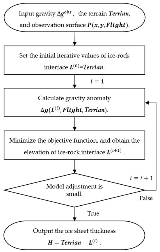
Figure 2.
A flow chart of the interface inversion considering terrain and UOSs simultaneously.
3. Synthetic Examples
In this section, the proposed method is applied to two groups of synthetic models. And all the synthetic models are generated by the numerical simulation of surfaces. To investigate the effectiveness of the presented method for a simple model, the smooth and regular reliefs of the surfaces (terrain, observation surface, and ice–rock interface) are designed in the first synthetic example. And the second synthetic example aims to demonstrate the validity of the proposed method for a complex model with random rough surfaces. To intuitively display the improvements of the proposed method, the results of the proposed method in two examples are compared with the results of the conventional inversion method.
3.1. Simple Synthetic Example
A series of simple and regular models were designed, as shown in Figure 2. In practical applications, the flight altitude often needs to be adjusted based on terrain variations to ensure the accuracy and precision of measurement data. Therefore, the flight altitude of airborne gravity is designed to be correlated with the terrain. The elevations of the observation surface and terrain are shown in Figure 3a,b, respectively. We can see that the terrain is an asymmetrical mountain, and the observation surface has a similar shape. But the elevation of the observation surface is higher than the terrain, and their elevation parameters are shown in Table 1. As shown in Figure 3c, the ice–rock interface is a symmetrical valley with one depocenter. According to the elevations of the terrain and ice–rock interface, we can obtain the ice sheet thickness shown in Figure 3d. The shape of the ice-rock interface is simple and asymmetrical, and its density contrast is set as . This density contrast is the difference between ice density and the average density of the crust. As shown in Table 1, the range of the ice sheet thickness is from m to m, and the mean thickness is m. The gravity anomaly of this group model (Figure 3e) is generated on a grid with points and a 500 m interval. It is obvious that there is no direct correlation between the gravity anomaly and ice sheet thickness.
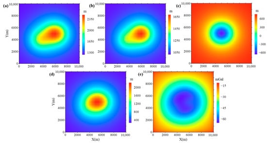
Figure 3.
The models and gravity anomaly in synthetic example 1: (a) The elevation of observation surface. (b) The elevation of terrain. (c) The elevation of ice–rock interface. (d) The ice sheet thickness. (e) The theoretical gravity anomaly due to these models.

Table 1.
Parameters of the models and gravity anomaly in synthetic example 1.
At first, the conventional inversion method without considering the terrain and observation surface is applied for comparison. And the calculated plane of the conventional inversion method is on plane . Figure 4a shows the calculated gravity anomaly of the estimated ice thickness (in Figure 4c) obtained from the conventional inversion method. For ease of comparison, the same color bar as Figure 3e is used in Figure 4a, and the color bar in Figure 4c is also the same as in Figure 3d. As we can see, the shape of the calculated gravity anomaly (Figure 4a) is close to the theoretical gravity anomaly (Figure 3e), but there is a significant morphological difference between the estimated ice thickness (Figure 4c) and the theoretical ice thickness. In addition, the residuals of data fitting and the residuals of estimated ice thickness are shown in Figure 4b,d, respectively. We can find out that the large deformation of the estimated ice thickness is negatively correlated with the morphology of the terrain and observation surface (Figure 3a,b). Combining the data in Table 2, the large residuals of the ice thickness can reach m, while the data misfit is only mGal.
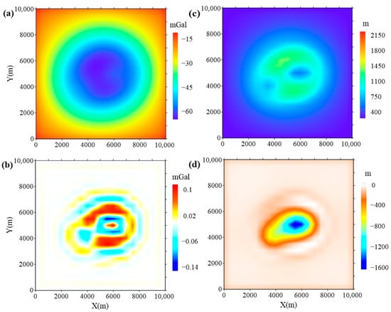
Figure 4.
The results of the simple models obtained by the conventional method: (a) The calculated gravity anomaly. (b) The residuals of data fitting. (c) The estimated ice thickness. (d) The residuals between the inverted thickness and the true value.

Table 2.
Statistical misfit comparison between w/o considering the terrain and UOSs of synthetic example 1.
Then, the presented inversion method considering the terrain and UOSs is applied. The results of the simple models obtained by the proposed inversion method are shown in Figure 5. As shown in Figure 5a,b, this inversion fits the data well. The estimated ice thickness shown in Figure 5c is obtained by subtracting the elevation of the ice–rock interface from the elevation of the terrain (Figure 3b), and the residuals of the thickness are shown in Figure 5d. Similarly, the color bars in Figure 5a,c are modified to be the same as those in Figure 3e,d. It is obvious that the shape of the estimated thickness obtained by the proposed method is similar to the theoretical model, and the amplitude of the estimated result is close to the true value. With the set color bars in Figure 5b,d being the same as those in Figure 4b,d, the comparisons of the residuals between the proposed method and the conventional inversion method are more intuitive. And, as shown in Table 2, the improvements of the presented method are quantified. The numerical interval for the residuals of the estimated ice thickness is reasonable, which is m. Overall, the proposed method can obtain better results, and the reliefs of the terrain and observation surface have a significant negative impact on the estimation of ice thickness.

Figure 5.
The results of the simple models obtained by the proposed method: (a) The calculated gravity anomaly. (b) The residuals of data fitting. (c) The estimated ice thickness. (d) The residuals between the inverted thickness and the true value.
3.2. Complex Synthetic Example
In this example, a series of complex and irregular models are built to validate the ability of the proposed method to estimate the random rough surfaces. As shown in Figure 6b, the terrain exhibits a bimodal shape, with one larger and one smaller protrusion. And the shapes of the observation surface (Figure 6a) and the terrain are approximately similar, but the terrain is more random. But, as shown in Table 3, the elevation of the observation surface is higher than the terrain. These are designed based on geological knowledge. As shown in Figure 6c, the ice–rock interface is a random and rough surface. Utilizing the elevations of the terrain and ice–rock interface, the ice sheet thickness is obtained (Figure 6d). The range of the ice sheet thickness is m, and the average thickness is m. And the density contrast of the ice–rock interface is also set as g/cm3. The gravity anomaly of this group model (Figure 6e) is calculated at the nodes of a grid with a 500 m grid step. And the relationship between the gravity anomaly and ice sheet thickness is also invisible.
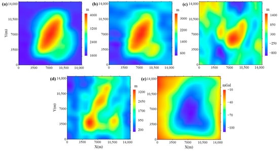
Figure 6.
The models and gravity anomaly in synthetic example 2: (a) The elevation of observation surface. (b) The elevation of terrain. (c) The elevation of ice–rock interface. (d) The ice sheet thickness. (e) The theoretical gravity anomaly due to these models.

Table 3.
Parameters of the models and gravity anomaly in synthetic example 2.
The results of the complex models obtained by the conventional inversion method are shown in Figure 7. And the calculated plane of the conventional inversion method is on plane . For ease of comparison, the color bars of the results in Figure 7a,c are modified to be the same as those in Figure 6e,d. It can be seen that the calculated gravity anomaly (Figure 7a) fits the theoretical gravity anomaly (Figure 6e) well, but there are some large deformations of the estimated ice thickness (Figure 7c) compared with the theoretical ice thickness (Figure 6d). And the terrain and observation surface (Figure 6a,b) have a complex impact on the estimated thickness of the conventional method. As shown in Table 4, the large residuals of the ice thickness are in the range of m.
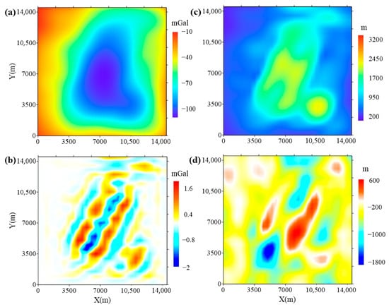
Figure 7.
The results of the complex models obtained by the conventional method: (a) The calculated gravity anomaly. (b) The residuals of data fitting. (c) The estimated ice thickness. (d) The residuals between the inverted ice thickness and the true value.

Table 4.
Statistical misfit comparison between w/o considering the terrain and UOSs of synthetic example 2.
Subsequently, the presented method is applied to the complex models. As shown in Figure 8a,b, the calculated gravity anomaly fits well. Subtracting the elevation of the ice–rock interface from the elevation of the terrain (Figure 6b), the estimated ice thickness shown in Figure 8c is obtained. In order to display the improvements of the proposed method more intuitively, the color bars in Figure 8a,c are set to be the same as those in Figure 6e,d and Figure 8b,d, as well as Figure 7b,d. As we can see, the estimated thickness is very close to the theoretical model. But there still exist some reasonable residuals. And as shown in Table 4, the residuals of the estimated ice thickness are in the range of m. Although the surfaces are complex and irregular, the proposed method can also obtain good results.
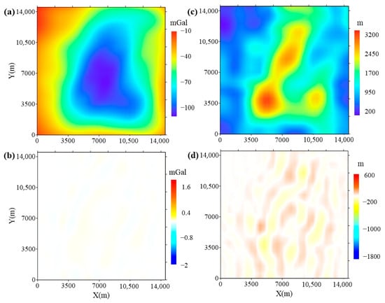
Figure 8.
The results of the complex models obtained by the proposed method: (a) The calculated gravity anomaly. (b) The residuals of data fitting. (c) The estimated ice thickness. (d) The residuals between the inverted thickness and the true value.
4. Real Data Application
To investigate the practicality of the proposed method, we applied it to a region in Antarctica. As shown in Figure 9, the study area is located in East Antarctica. And it is entirely buried under a thick ice sheet. Antarctica’s Gamburtsev Province (AGAP) Project collected the airborne geophysical data in this region. According to the inputs of the presented method, the aerogravity data [23] and radio-echo sounding data [24] from the AGAP are utilized (Figure 10). The residual gravity anomaly caused by the ice–rock interface is shown in Figure 10a, and the aircraft altitude of the aerogravity is shown in Figure 10b. Based on the radio-echo sounding data, we can obtain the elevation of the ice surface (Figure 10c), the derived ice bed elevation (Figure 10d), the and ice thickness (Figure 10e). The elevation of the ice surface is the important input of the presented method. And the radar-derived ice bed elevation and ice thickness are used to verify the accuracy of inversion results. Integrating the analysis of Table 5, it can be found that the reliefs of the aircraft altitude and ice surface elevation in this region are relatively moderate. Therefore, there is a discernible correlation between the shapes of the residual gravity anomaly and the ice bed elevation. Moreover, the range of the radar-derived ice sheet thickness is m, and the average thickness is m.
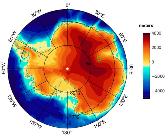
Figure 9.
Location of the study area in Antarctica. The base map is the elevation of the Antarctic topography. The study area is bounded by a green rectangle.
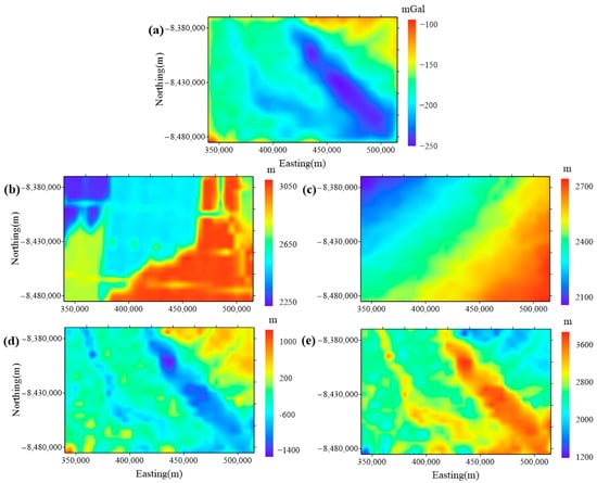
Figure 10.
The airborne geophysical data from the AGAP Project. Aerogravity data: (a) the residual gravity anomaly caused by the ice–rock interface; (b) the aircraft altitude. Radio-echo sounding data: (c) ice surface elevation, (d) ice bed elevation, and (e) ice thickness.

Table 5.
Parameters of the airborne geophysical data from the AGAP Project.
The results obtained by the conventional method in the survey area are shown in Figure 11. And the calculated plane of the conventional inversion method is on plane . To facilitate comparison, the color bars in Figure 11a,c are adjusted to match those in Figure 10a,e. It can be seen that the calculated gravity anomaly (Figure 11a) fits the residual gravity anomaly (Figure 10a) well. But compared with the radar-derived thickness (Figure 10e), notable deviations exist in the estimated ice thickness (Figure 11c). And the estimated thickness of the conventional method is influenced by both the ice surface and aircraft altitude (Figure 10b,c). The large deviations (Figure 11d) are distributed in locations where the ice surface and aircraft altitude fluctuate greatly. As shown in Table 6, the large residuals of the ice thickness are in the range of m.
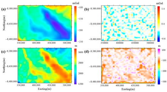
Figure 11.
The results obtained by the conventional method in the survey area: (a) The calculated gravity anomaly. (b) The residuals of data fitting. (c) The estimated ice thickness. (d) The residuals between the estimated ice thickness and the radar-derived ice thickness.

Table 6.
Statistical misfit comparison between w/o considering the terrain and UOSs of the survey area.
Then, the proposed method is applied to the survey area. As shown in Figure 12a,b, the calculated gravity anomaly fits well. By subtracting the elevation of the ice–rock interface from the elevation of the ice’s surface (Figure 10c), we obtain the estimated ice thickness shown in Figure 12c. To present the advancements of the proposed method in a more visual manner, the color bars in Figure 12a,c are aligned with those in Figure 10a,e. Similarly, the color bars in Figure 12b,d are matched to those in Figure 11b,d. As we can observe, the estimated thickness is very close to the radar-derived values. However, there are still some reasonable residuals present. And the residuals of the estimated ice thickness (Table 6) are in the range of m. The application of the real data from East Antarctica shows that our proposed method considering terrain and UOSs can fade the negative influence of terrain and UOSs in density interface inversion.
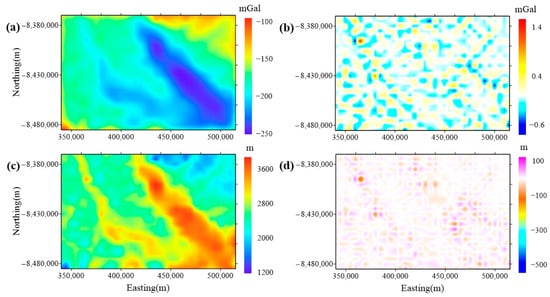
Figure 12.
The results obtained by the proposed method in the survey area: (a) The calculated gravity anomaly. (b) The residuals of data fitting. (c) The estimated ice thickness. (d) The residuals between the inverted thickness and the radar-derived value.
5. Conclusions
In this study, we propose an improved 3D density interface inversion method simultaneously considering terrain and UOSs to estimate ice sheet thickness. The synthetic examples validate the effectiveness of the presented method. And the results of the conventional method in the simple synthetic example intuitively display that the reliefs of the terrain and observation surfaces have a significant negative impact on the estimation of ice thickness. Furthermore, in the complex synthetic example, even though the terrain and UOSs are complex and irregular, the proposed method can still obtain good results.
The real data application in East Antarctica confirms the practicality of the proposed method for estimating ice sheet thickness. Utilizing the aerogravity data and radio-echo sounding data from the AGAP, the ice sheet thickness obtained by the proposed method is very close to the radar-derived ice thickness. Compared with the conventional method, the proposed method fades the deviations caused by the fluctuations of the ice surface and aircraft altitude.
Overall, the proposed method avoids the distortion and instability caused by the terrain and the UOSs and improves the accuracy of estimating ice sheet thickness with airborne gravity. Still, some limitations should also be mentioned. Because of the inherent nonuniqueness of gravity inversion, there exist some reasonable residuals of the estimated ice thickness. Some prior depth points are suggested to be introduced to improve the accuracy of the estimation. And the computational cost of the proposed method may be a bit high when the number of computational grids is large.
Author Contributions
Conceptualization and methodology, Y.L., J.W. and F.L.; visualization and writing—original draft preparation, Y.L. and J.W.; writing review and editing, Y.L., J.W., F.L. and X.M. All authors have read and agreed to the published version of the manuscript.
Funding
This research was funded by the National Key R&D Program of China, grant number 2022YFC2807404.
Data Availability Statement
The aerogravity data and radio-echo sounding data in East Antarctic presented in this paper are available upon request from the British Antarctic Survey at https://www.bas.ac.uk/ (accessed on 27 March 2024).
Acknowledgments
We acknowledge all members of the AGAP project team for their great contributions to the collection and processing of the airborne gravity data and radio-echo sounding data in the GSM.
Conflicts of Interest
The authors declare no conflicts of interest.
References
- Bamber, J.L.; Layberry, R.L.; Gogineni, S.P. A new ice thickness and bed data set for the Greenland ice sheet: 1. Measurement, data reduction, and errors. J. Geophys. Res. Atmos. 2001, 106, 33773–33780. [Google Scholar] [CrossRef]
- Yang, T.; Liang, Q.; Zheng, L.; Li, T.; Chen, Z.; Hui, E.; Cheng, X. Mass Balance of the Antarctic Ice Sheet in the Early 2lst Century. Remote Sens 2023, 15, 1677. [Google Scholar] [CrossRef]
- Corbató, C.E. Thickness and Basal Configuration of Lower Blue Glacier, Washington, Determined by Gravimetry. J. Glaciol. 1965, 5, 637–650. [Google Scholar] [CrossRef]
- Millan, R.; Rignot, E.; Rivera, A.; Martineau, V.; Mouginot, J.; Zamora, R.; Uribe, J.; Lenzano, G.; De Fleurian, B.; Li, X.; et al. Ice thickness and bed elevation of the Northern and Southern Patagonian Icefields. Geophys. Res. Lett. 2019, 46, 6626–6635. [Google Scholar] [CrossRef]
- MacGregor, J.A.; Colgan, W.T.; Paxman, G.J.G.; Tinto, K.J.; Csathó, B.; Darbyshire, F.A.; Fahnestock, M.A.; Kokfelt, T.F.; MacKie, E.J.; Morlighem, M.; et al. Geologic provinces beneath the Greenland Ice Sheet constrained by geophysical data synthesis. Geophys. Res. Lett. 2024, 51, e2023GL107357. [Google Scholar] [CrossRef]
- Stevens, C.W.; Moorman, B.J.; Solomon, S.M.; Hugenholtz, C.H. Mapping subsurface conditions within the near-shore zone of an Arctic delta using ground penetrating radar. Cold Reg. Sci. Technol. 2009, 56, 30–38. [Google Scholar]
- Fretwell, P.; Pritchard, H.D.; Vaughan, D.G.; Bamber, J.L.; Barrand, N.E.; Bell, R.; Bianchi, C.; Bingham, R.G.; Blankenship, D.D.; Casassa, G.; et al. Bedmap2: Improved ice bed, surface and thickness datasets for Antarctica. Cryosphere 2013, 7, 375–393. [Google Scholar] [CrossRef]
- Liu, J.; Wang, S.; He, Y.; Li, Y.; Wang, Y.; Wei, Y.; Che, Y. Estimation of ice thickness and the features of subglacial media detected by ground penetrating radar at the Baishui River Glacier No. 1 in Mt, Yulong, China. Remote Sens 2020, 12, 4105. [Google Scholar] [CrossRef]
- Jin, H.; Yao, X.; Wei, Q.; Zhou, S.; Zhang, Y.; Chen, J.; Yu, Z. Ice Thickness Assessment of Non-Freshwater Lakes in the Qinghai-Tibetan Plateau Based on Unmanned Aerial Vehicle-Bornelce-Penetrating Radar: A Case Study of Qinghai Lake and Gahai Lake. Remote Sens 2024, 16, 959. [Google Scholar] [CrossRef]
- Yan, J.; Lü, Q.; Luo, F.; Cheng, S.; Zhang, K.; Zhang, Y.; Xu, Y.; Zhang, C.; Liu, Z.; Ruan, S.; et al. A gravity and magnetic study of lithospheric architecture and structures of South China with implications for the distribution of plutons and mineral systems of the main metallogenic belts. J. Asian Earth Sci. 2021, 221, 104938. [Google Scholar] [CrossRef]
- Liu, Y.; Huang, Y.; Lü, Q.; Liu, S. Adaptive mesh-free approach for gravity inversion using modified radial basis function. IEEE Trans. Geosci. Remote Sens. 2023, 61, 5907612. [Google Scholar] [CrossRef]
- Bull, C.; Hardy, J.R. The Determination of the Thickness of a Glacier from Measurements of the Value of Gravity. J. Glaciol. 1956, 2, 755–763. [Google Scholar] [CrossRef]
- Thiel, E.; Lachapelle, E.; Behrendt, J. The Thickness of Lemon Creek Glacier, Alaska, As Determined by Gravity Measurements. Eos Trans. Am. Geophys. Union 1957, 38, 745. [Google Scholar]
- Parker, R.L. The rapid calculation of potential anomalies. Geophys. J. Int. 1973, 31, 447–455. [Google Scholar] [CrossRef]
- Gourlet, P.; Rignot, E.; Rivera, A.; Casassa, G. Ice thickness of the northern half of the Patagonia Icefields of South America from high-resolution airborne gravity surveys. Geophys. Res. Lett. 2016, 43, 241–249. [Google Scholar] [CrossRef]
- An, L.; Rignot, E.; Milan, R.; Tinto, K.; Willis, J. Bathymetry of northwest Greenland using ocean melting Greenland (OMG) high-resolution airborne gravity and other data. Remote Sens. 2019, 11, 131. [Google Scholar] [CrossRef]
- Eisermann, H.; Eagles, G.; Jokat, W. Coastal bathymetry in central Dronning Maud Land controls ice shelf stability. Sci. Rep. 2024, 14, 1367. [Google Scholar] [CrossRef] [PubMed]
- Yao, C.; Huang, W.; Guan, Z. Fast splines conversion of curved-surface potential field and vertical gradient data into horizontal-plane data. Oil Geophys. Prospect. 1997, 32, 229–236. [Google Scholar]
- Pilkington, M.; Boulanger, O. Potential field continuation between arbitrary surfaces—Comparing methods. Geophysics 2017, 82, J9–J25. [Google Scholar] [CrossRef]
- Jekeli, C. The downward continuation of aerial gravimetric data without density hypothesis. Bull. Geod. 1987, 61, 319–329. [Google Scholar] [CrossRef]
- Yang, J.; Jekeli, C.; Liu, L. Seafloor topography estimation from gravity gradients using simulated annealing. J. Geophys. Res. Solid Earth 2018, 123, 6958–6975. [Google Scholar] [CrossRef]
- Tikhonov, A.N.; Arsenin, V.Y. Solutions of Ill-Posed Problems; V. H. Winston & Sons: Washington, DC, USA, 1977. [Google Scholar]
- Ferraccioli, F.; Finn, C.; Jordan, T.A.; Bell, R.E.; Anderson, L.M.; Damaske, D. East Antarctic rifting triggers uplift of the Gamburtsev Mountains. Nature 2011, 479, 388–392. [Google Scholar] [CrossRef] [PubMed]
- Bell, R.E.; Ferraccioli, F.; Creyts, T.T.; Braaten, D.; Corr, H.; Das, I.; Damaske, D.; Frearson, N.; Jordan, T.; Rose, K.; et al. Widespread Persistent Thickening of the East Antarctic Ice Sheet by Freezing from the Base. Science 2011, 331, 1592–1595. [Google Scholar] [CrossRef] [PubMed]
Disclaimer/Publisher’s Note: The statements, opinions and data contained in all publications are solely those of the individual author(s) and contributor(s) and not of MDPI and/or the editor(s). MDPI and/or the editor(s) disclaim responsibility for any injury to people or property resulting from any ideas, methods, instructions or products referred to in the content. |
© 2024 by the authors. Licensee MDPI, Basel, Switzerland. This article is an open access article distributed under the terms and conditions of the Creative Commons Attribution (CC BY) license (https://creativecommons.org/licenses/by/4.0/).