Abstract
Digital elevation models (DEMs) are widely used in digital terrain analysis, global change research, digital Earth applications, and studies concerning natural disasters. In this investigation, a thorough examination and comparison of five open-source DEMs (ALOS PALSAR, SRTM1 DEM, SRTM3 DEM, NASADEM, and ASTER GDEM V3) was carried out, with a focus on the Chongqing region as a specific case study. By utilizing ICESat-2 ATL08 data for validation and employing a random forest model to refine terrain variables such as slope, aspect, land cover, and landform type, a study was undertaken to assess the precision of DEM data. Research indicates that spatial resolution significantly impacts the accuracy of DEMs. ALOS PALSAR demonstrated satisfactory performance, reducing the corrected root mean square error (RMSE) from 13.29 m to 9.15 m. The implementation of the random forest model resulted in a significant improvement in the accuracy of the 30 m resolution NASADEM product. This improvement was supported by a decrease in the RMSE from 38.24 m to 9.77 m, demonstrating a significant 74.45% enhancement in accuracy. Consequently, the ALOS PALSAR and NASADEM datasets are considered the preferred data sources for mountainous urban areas. Furthermore, the study established a clear relationship between the precision of DEMs and slope, demonstrating a consistent decline in precision as slope steepness increases. The influence of aspect on accuracy was considered to be relatively minor, while vegetated areas and medium-to-high-relief mountainous terrains were identified as the main challenges in attaining accuracy in the DEMs. This study offers valuable insights into selecting DEM datasets for complex terrains in mountainous urban areas, highlighting the critical importance of choosing the appropriate DEM data for scientific research.
1. Introduction
Digital elevation models (DEMs) are essential datasets for analyzing the heights and features of the Earth’s surface. DEMs are extensively used in agricultural terrain suitability studies, topographic mapping, the distribution of climatic elements, hydrological modeling, and urban planning [1,2,3,4]. DEMs have become essential variables in the creation of land-use and land-cover maps on sloping terrains using machine learning and deep learning techniques. The creation of DEM datasets involves various technical methods [5], such as ground-based field surveys [6], digital topographic maps [7], stereophotogrammetry [8], Interferometric Synthetic Aperture Radar (InSAR) [9], and Airborne Light Detection and Ranging (LiDAR) scanning [10].
With the continuous advancement of remote sensing and Earth observation technologies, the development of large-area, high-resolution DEMs has become crucial. Over the years, the development of these technologies has resulted in a variety of global open-source digital elevation model data products. Examples include the L-band interferometric SAR-based ALOS PALSAR [11], the Space Shuttle Radar Topography Mission SRTM, generated using SAR interferometry [12], the Advanced Spaceborne Thermal Emission and Reflection Radiometer (ASTER) Global Digital Elevation Model (GDEM) [13], and the TanDEM-X DEM [14], which was obtained from radar satellite interferometry. These open-source DEMs provide valuable and extensive data sources for researchers, enhancing understanding of the Earth’s surface in developing countries, particularly in regions with limited geospatial infrastructure.
However, it is crucial to assess the accuracy of global open-source DEMs. Despite their high accuracy potential, models are still only approximations of reality. Due to differences in imaging configurations and data processing methods, the quality of DEMs can vary depending on terrain conditions and land-cover types, leading to inherent errors [15]. These errors have significant implications for various applications of DEMs [16,17,18]. Therefore, accurate elevation data are essential for various applications like terrain analysis, hydrological modeling, decision support, risk assessment, and algorithm enhancement. By assessing the accuracy of DEMs, it is possible to determine if data can be trusted in specific scenarios, improving the reliability of decision making and applications. Furthermore, accuracy assessments can refine DEM generation algorithms, enhancing the quality and precision of the resulting DEM. Therefore, when selecting DEM data, it is essential to consider their accuracy to enhance the quality of experiments, support geographical research, and ensure precision. Conducting accuracy assessments of global free open-source DEMs is crucial to ensure data reliability and effective application.
Currently, the assessment of DEMs for accuracy has become an important area of focus for researchers [19]. One common method for assessing the accuracy of open-source DEM datasets is the traditional method [20] of comparing DEM data with precise Ground Control Points (GCPs). However, traditional field measurement methods for obtaining highly accurate GCPs are both time-consuming and costly, and thus they no longer meet the demands of current accuracy assessments and stereoscopic mapping tasks. In 2003, the Ice, Cloud, and Land Elevation Satellite (ICESat) was launched with the Geoscience Laser Altimeter System [12], making it the first satellite with a laser altimetry system. GLAS emitted laser footprints on the Earth’s surface with a 70 m diameter and 170 m spacing at a 40 kHz frequency. The GLAS system demonstrated high accuracy, with planimetric accuracy at the order of 10 m and vertical accuracy ranging from 0.12 m to 0.50 m [21,22]. Therefore, ICESat/GLAS provides high-precision global elevation data and has been used as a data source for global GCPs [23,24]. On 15 September 2018, the Ice, Cloud, and Land Elevation Satellite-2 (ICESat-2) was successfully launched, equipped with the Advanced Topographic Laser Altimeter System (ATLAS). The ATLAS system reduced the footprint size from 70 m to 17 m, decreased the spacing between footprints from 150 m to 0.7 m, and increased the operating frequency to 10 kHz compared to GLAS, allowing for denser data points. This enables ATLAS to capture almost continuous surface profiles of the Earth’s surface. Consequently, ATLAS effectively captures complex changes in mountainous terrain and resists slope effects, achieving higher precision in mountain measurements.
Research indicates that ICESat-2/ATLAS exhibits higher accuracy. For example, Wang [25] validated the surface elevation of ICESat-2’s Level-2 product ATL03 in the United States using LiDAR data, with an average error of -0.61 m. ATL08, being a more advanced product compared to ATL03, offers data on both terrain and canopy height. Neuenschwander [26] comprehensively validated the horizontal positioning and vertical elevation accuracy of single-track ATL08 data. The results showed that the horizontal positioning offset was 5 m, which falls within the 6.5 m horizontal positioning accuracy range described by ICESat-2/ATLAS. The accuracies of extracting ground elevation and canopy height vertically were 0.85 m and 3.2 m, respectively. Subsequently, Neuenschwander et al. [27] collected ATL08 data in the Finland region for 11 months and validated the accuracy of the data using LiDAR data as a reference. The results showed that the ground elevation extraction error by ATL08 was under 0.75 m, and the canopy height extraction error was 0.56 m. Therefore, ICESat-2 is precise enough to be used as a high-precision ground control point data source for evaluating and improving global open-source DEM data products [28,29,30].
In recent years, many studies have been dedicated to reducing errors in DEMs. However, most current methods for eliminating errors in DEMs rely on traditional approaches, such as improving data collection methods and utilizing high-precision altimetry satellites [31,32,33]. Nevertheless, these methods are often costly and limited to relatively small areas, making them impractical for large-scale regions. Machine learning, especially neural networks, is a mature technology widely used for tasks such as regression analysis and prediction because of its powerful computational capabilities. Therefore, techniques such as machine learning and neural networks have the potential to enhance and improve the accuracy of DEM data. Currently, there are primarily two methods for improving the quality of DEM data. The first involves using artificial intelligence technologies, such as machine learning and neural networks, to enhance the accuracy of existing DEM data [34,35]. The second method involves utilizing multi-source DEM data and merging existing DEM data by calculating weighting coefficients [36].
Chongqing’s complex mountainous terrain and frequent cloud cover create a diverse landscape with mountains, hills, and river valleys. Due to this significant spatial variability, assessing the accuracy of DEMs in Chongqing poses challenges and practical implications. Therefore, this study compares five open-source DEM datasets (ALOS PALSAR, SRTM1 DEM, SRTM3 DEM, NASADEM, and ASTER GDEM V3) using terrain elevation information derived from ICESat-2 ATL08 laser altimetry data to accurately depict the terrain of Chongqing and provide support for various Earth science research endeavors. The study evaluates whether these DEMs exhibit limitations or peculiarities in vertical accuracy in the typical mountainous regions with frequent cloud cover in China (Chongqing). The aim is to provide useful guidance for other researchers using these DEMs in similar terrain conditions.
The structure of this article is as follows. Section 2 provides an overview of the research area, datasets, and research methods. Specifically, this section outlines the preprocessing of ICESat-2 ATL08 data, introduces evaluation metrics and terrain factors, explains the prediction process of the random forest model, and presents a flowchart of the article’s research content. Section 3 provides quality assessments and analysis results before and after corrections. Section 4 discusses how various terrain factors affect the accuracy of DEMs and the selection of DEMs for mountainous urban areas. Section 5 summarizes the conclusions of the entire article.
2. Materials and Methods
2.1. Study Area
Chongqing, situated in the southeastern part of China, serves as a transitional area between the Qinghai–Tibet Plateau and the middle and lower reaches of the Yangtze River Plain (Figure 1). The region spans from approximately 105°11′ to 110°11′ east longitude and 28°10′ to 32°13′ north latitude, covering a total area of approximately 82,400 square kilometers. Chongqing’s terrain combines mountains, river valleys, and hilly areas. The diverse and intricate terrain pattern in this area makes it ideal for evaluating various DEM products. Therefore, this region is highly effective for evaluating the accuracy of various DEM products.
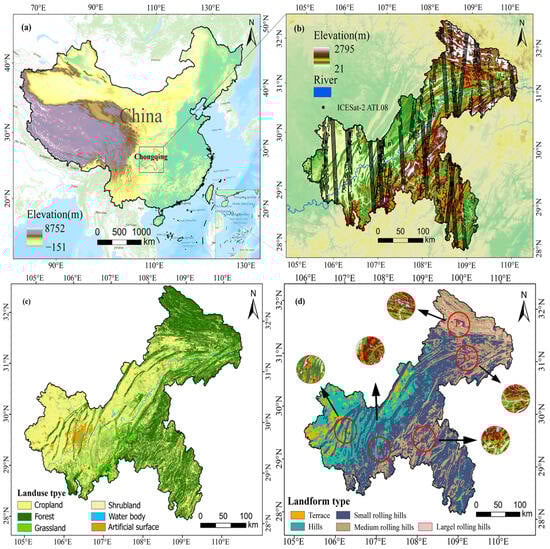
Figure 1.
Study area and ICESat-2 ATL08 tracks. (a) The location of the study area. (b) The overall tracks of ICESat-2 ATL08; the black dots represent the laser footprint of the ICESat-2 satellite on the ground. (c) Land-cover type. (d) Landform type: A–E represent, respectively, terrace, hills, small rolling hills, medium rolling hills, and large rolling hills.
2.2. Data
This study compared five commonly used open-source DEM datasets. The DEM datasets were ALOS PALSAR, SRTM1 DEM, SRTM3 DEM, NASADEM, and ASTER GDEM V3. Table 1 provides basic information on the DEMs and their publicly accessible sources.

Table 1.
Basic parameters of five open-source DEM data products used in this study.
2.2.1. ALOS PALSAR
ALOS PALSAR data are sourced from a satellite launched by the Japan Aerospace Exploration Agency (JAXA) in May 2006. It carries the Phased Array L-band Synthetic Aperture Radar. The primary goal of PALSAR is to provide global land-coverage information, including terrain elevation data. The data have a spatial resolution of 12.5 m and utilize the L-band frequency, providing high-resolution surface observation capabilities that are effective in all weather conditions and can operate day and night.
2.2.2. SRTM DEM
The SRTM1 and SRTM3 datasets originate from the Space Shuttle Radar Topography Mission, which was launched in February 2000. This mission utilized InSAR to produce two land elevation data products with different spatial resolutions. The U.S. product has a spatial resolution of 1 arc second (30 m), while the global product has a resolution of 3 arc seconds (90 m). They cover about 80% of the Earth’s land surface, ranging from 60° north latitude to 56° south latitude. The SRTM sensor uses C-band SAR to measure the heights of ground and non-ground features on the Earth’s surface. According to the SRTM mission objectives, the SRTM DEM is expected to have a linear vertical absolute height error of around 16 m and a linear vertical relative height error of 10 m [13]. This article uses the latest version data of V003 (30 m) and V4.1 (90 m) released in 2014 and 2015.
2.2.3. NASADEM
The NASADEM dataset, released in February 2020, is derived from the original SRTM data through secondary processing with additional datasets such as ASTER GDEM, PRISM, ICESat, and GLAS, providing a 30 m spatial resolution. The main goal is to enhance geographic positioning accuracy by addressing gaps and limitations in the SRTM dataset [37]. The development team utilized ICESat data to conduct a quantitative evaluation in Canada and found that the vertical accuracy of the data was 5.3 m [38], and 6.59 m in China [39].
2.2.4. ASTER GDEM V3
The ASTER GDEM project is a collaboration between NASA and the Ministry of Economy, Trade, and Industry (METI) of Japan. It uses stereophotogrammetry from orbit to create near-infrared images spanning latitudes from 83°N to 83°S. ASTER GDEM has had three versions, with the latest upgrade being ASTER GDEM V3, which was released on 5 August 2019. This version incorporates 360,000 pairs of optical stereo data to reduce elevation discrepancies and anomalies in water bodies. Previous studies indicate a slight improvement in vertical accuracy using ASTER GDEM V3, with RMSE ranging from 6.92 m to 9.25 m across different land-cover types in the United States [40].
2.2.5. ICESat-2 ATL08 Data
NASA’s ICESat-2, a satellite-borne laser satellite carrying the Advanced Topographic Laser Altimeter System (ATLAS), released on 15 September 2018, is a follow-up mission to ICESat. ATLAS can emit three pairs of laser beams with a 532 nm wavelength at a 10 kHz pulse repetition rate. Each overlapping footprint has a diameter of approximately 17 m, with a spacing of about 0.7 m between orbits. Each pair of beams consists of a strong beam and a weak beam, with a strong-to-weak energy ratio of 4:1, spaced approximately 3.3 km apart, with a 90 m spacing per pair [41]. Consequently, ICESat-2 demonstrates significant enhancements in data coverage density, data accuracy, and spatial resolution. Additionally, ICESat-2 demonstrates strong resistance to slope effects, enabling more precise measurements of mountainous terrain [27,42,43].
Data collected by ATLAS are processed into 22 products (ATL00-ATL21). Among these, ATL08 products are derived from ATL03 (global geolocated photon cloud) and provide global coverage of terrain and canopy height data. ATL08 provides height information (h_te_interp) at 100 m intervals, along with the most suitable terrain elevation (h_te_bestfit) at the midpoint of each 100 m segment [44]. Due to the inclusion of detailed parameters like latitude, longitude, slope, cloud cover, acquisition time, terrain, and canopy information, ATL08 is a crucial source of information for control points. Previous studies have shown that the vertical accuracy of ground elevation in ATL08 data is 0.75 m [27], making it a suitable reference for surface elevation.
As ground and vegetation reflectance is low, the return signal in remote sensing data mainly originates from the strong beam, which provides more accurate ground elevation precision than the weak beam. Therefore, our experimental data consist solely of strong beam trajectories. Additionally, there is a significant amount of noise photons during data acquisition, with background noise in night-time data notably lower than during the daytime. Hence, data filtering is performed using night flags (night_flag), cloud flags (cloud_flag_atm), and low slope information (terrain_slope) to ensure reliable ground elevation information is obtained [45,46,47].
2.2.6. GlobeLand30
GlobeLand30, a global surface coverage dataset with 30 m spatial resolution, developed in China, was initially released in 2014 for the 2000 and 2010 editions. The Ministry of Natural Resources (MNR) updated the dataset in 2017 to create the 2020 edition. This product utilizes existing land-cover data, global MODIS NDVI data, global basic geographic information data, global DEMs, and online high-resolution imagery to assist in sample selection and auxiliary classification. It has been reported that the overall accuracy of this dataset is 85.72%. Considering that land cover has different effects on the reflection, absorption, and scattering characteristics of the Earth’s surface, utilizing land-cover data can help evaluate and enhance DEM elevation products. Therefore, in our study, we utilized both the 2010 and 2020 versions of the GlobeLand30 dataset.
2.3. Methods
2.3.1. Pre-Processing of ICESat-2 ATL08 Data
Initially, elevation data (Table 2) were extracted from the original HDF5 files of ATL08 using Python (v3.9.12). We extracted the laser point data for Chongqing City for the entire year of 2020, totaling 74,972 control points. Previous studies [48,49] have indicated that ATLAS photon data may be influenced by various factors such as slope, cloud cover, and imaging time. These factors can lead to a reduction in photon energy and introduce errors in distance measurements. Among these factors, slope has a particularly significant impact on elevation accuracy, with accuracy decreasing significantly as slope increases. Additionally, elevation accuracy is typically higher during night-time observations, and clearer skies also reduce photon obstructions, thereby improving accuracy.
Table 2.
Descriptions of ATL08 data product parameters.
We set filtering thresholds based on relevant criteria, such as “terrain_slope < 0.01”, “cloud_flag_atm < 2”, and “night_flag = 1”. After a series of meticulous filtering rounds, the dataset was reduced to 51,642 control points. To enhance the credibility of the results and ensure the accuracy of the elevation data, we calculated the height differences (Δh) between each ground control point and all DEM datasets. Points with height differences exceeding ±100 were identified as outliers and removed. Ultimately, we obtained 50,998 high-quality control points that met the experimental criteria.
Due to differences in vertical reference systems and spatial resolutions among the five DEM datasets, there may be discrepancies in elevation information. Before extracting elevation data, it is essential to standardize the vertical reference systems of all datasets. We converted orthometric heights (EGM96) to ellipsoidal heights (WGS84) to eliminate errors from vertical datum differences. The conversion relationship is as follows:
In the equation, represents the ellipsoidal height, represents the orthometric height, and G denotes the difference between ellipsoidal height and orthometric height, which can be obtained from the ‘WG84.img’ file provided by ArcGIS 10.8.
Subsequently, we utilized bilinear interpolation to align DEM data with ICESat-2 laser data, ensuring consistency across various data sources. Through this process, we interpolated lower-resolution DEM data to match the spatial locations of the higher-resolution DEM data. This ensures data accuracy and reliability, establishing a strong foundation for further analysis and applications.
2.3.2. Assessment of Vertical Accuracy
Accurately speaking, all global open-source digital elevation models (DEMs) are digital surface models (DSMs) [33,50]. Typically, we uniformly consider them as DEMs. Therefore, in this paper, we will use the term “DEM” [51,52]. To comprehensively evaluate the differences in elevation distribution between ATL08 and the DEMs and measure the vertical accuracy of the DEMs, we selected four key evaluation metrics: mean error, mean absolute error, standard deviation, and root mean square error. Additionally, these metrics help us understand the accuracy of elevation data and provide detailed insights into errors. The specific formulas are as follows:
In the equations, represents the elevation value from ICESat-2, represents the elevation value from the DEM corresponding to each ICESat-2 laser point, and represents the difference in elevation between ICESat-2 and the DEM.
2.3.3. Elevation Accuracy Response Considering Different Slope, Aspect, Land Cover and Landform Types
In our study, slope, aspect, land cover, and terrain type are identified as crucial factors for evaluating the accuracy of global open-source DEMs. These factors are essential components of terrain data and are critical for various geographic information applications. Research has shown a positive correlation between slope and DEM accuracy [30]. Therefore, we categorized slope into five groups (≤5°, 5–10°, 10–15°, 15–20°, and ≥20°) to evaluate the effect of slope on DEM accuracy in mountainous urban areas. Aspect was divided into eight primary directions based on cardinal directions: north (337.5–22.5°), northeast (22.5–67.5°), east (67.5–112.5°), southeast (112.5–157.5°), south (157.5–202.5°), southwest (202.5–247.5°), west (247.5–292.5°), and northwest (292.5–337.5°).
To quantitatively assess the impact of land cover on DEM accuracy, we identified six land-cover categories from the 30 m GlobeLand30 data: cropland, forest, grassland, shrubland, water bodies, and artificial surfaces. Additionally, Chongqing is known as a “mountain city” because of its unique terrain features. Since terrain type is a crucial factor reflecting surface morphology, we identified six terrain types in the Chongqing region based on 1:1,000,000 topographic maps: plain, terrace, hills, small rolling hills, medium rolling hills, and large rolling hills. Considering terrain factors comprehensively enables a more thorough assessment of DEM data performance and applicability in specific geographic regions.
2.3.4. Random Forest Model
In this study, we utilized the random forest (RF) model to correct the five DEMs. Random forest is an ensemble learning algorithm based on decision trees and bagging, proposed by Breiman and Cutler in 2001 [53].
Compared to traditional decision tree models, the random forest model shows outstanding generalization ability. This method constructs multiple decision trees and combines their results through voting or averaging to decrease the model’s variance and improve stability [54]. Additionally, random forest reduces overfitting risk by randomly selecting feature subsets to build multiple decision trees. This process enhances generalization capability and improves robustness against outliers. Random forest has been shown in previous studies [34,55,56] to be a superior choice for DEM correction compared to other models like MLR, GRNN, BPNN, and GBT in predicting surface elevation.
We implemented the random forest model using the “Random Forest” package in the R programming language. We utilized 50,998 filtered ATL08 high-precision laser points as elevation data, randomly splitting them into a 70% training set and a 30% testing set to evaluate the accuracy improvements after correcting the five DEMs.
To achieve accurate random forest correction results, we established a mapping function to describe the relationship between seven factors: longitude, latitude, elevation, slope, aspect, land cover, terrain type, and ICESat-2 ATL08. The general relationship can be represented as follows:
In the equation, represent the mapping function used to quantitatively describe the functional relationship between the target variable and the feature variables. Here, represents the target variable, and represent the seven feature variables of longitude, latitude, elevation, slope, aspect, land cover, and terrain type. We denote the random forest model’s predictions for ICESat-2 ATL08 as the corrected elevation.
To determine the best parameter combination, we utilized the grid search method to perform three rounds of tuning for five parameters. These parameters were the number of trees (n_estimators), maximum depth (max_depth), minimum samples required to split a node (min_samples_split), minimum samples required at a leaf node (min_samples_leaf), and the maximum number of leaf nodes (max_leaf_nodes). The aim of adjusting parameters is to control the model’s complexity and performance to prevent overfitting. During the grid search parameter tuning process, cross-validation was used to evaluate each model’s performance and identify the best parameter combination to improve its generalization capability. Specifically, we utilized five-fold cross-validation for model evaluation to determine the best values for the five parameters. Additionally, we chose RMSE as the model’s loss function to evaluate its performance. The disparities between adjusted elevation and ICESat-2 ATL08 data aid in assessing a model’s fit and predictive accuracy. The process of evaluating and correcting the five DEMs’ accuracies is illustrated in Figure 2.
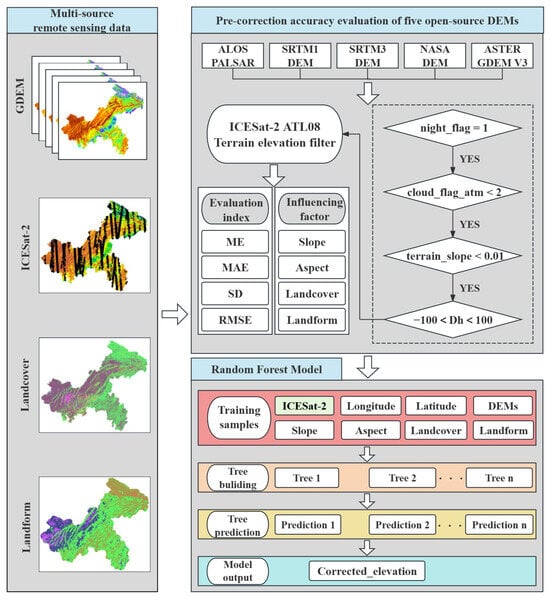
Figure 2.
Accuracy evaluation and correction flow chart of five DEMs using ICESat-2.
3. Results
3.1. Accuracy Evaluation of Five DEMs before and after Correction
For convenience, we will use the abbreviations ALOS, SRTM1, SRTM3, NASA, and ASTER to refer to ALOS PALSAR, SRTM1 DEM, SRTM3 DEM, NASADEM, and ASTER GDEM V3, respectively.
In this study, we first assessed elevation variations among the five DEMs to understand their accuracy before using the random forest model for correction. After analyzing the histograms (Figure 3), we found that the elevation variances of all five DEMs conformed to a normal distribution. Compared to the reference data from ICESat-2 ATL08, all five DEMs generally showed negative ME values, indicating a consistent elevation overestimation in the Chongqing region. Possible reasons for this result include (1) the complex terrain of the Chongqing region, especially in terrain depressions such as gorges and valleys, where satellite-measured elevation values may be lower than the actual ground elevation; (2) dense vegetation in the Chongqing region, which may affect the penetration and reflection of satellite radar signals, resulting in underestimated measurement results; and (3) terrain masking effects, where mountainous terrain may have shadowed areas, leading to weaker satellite signals and lower elevation measurements.
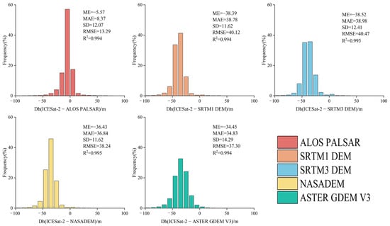
Figure 3.
Histogram of the elevation error for ALOS PALSAR, SRTM1 DEM, SRTM3 DEM, NASADEM, and ASTER GDEM V3.
All the DEMs showed a significant negative bias. ALOS demonstrated the best performance, with an ME of −5.57 m and an RMSE of 13.29 m, indicating a symmetrical distribution around zero. Conversely, SRTM3 performed the worst, with an ME of −38.52 m and an RMSE of 40.47 m. The accuracy ranking of the other three DEMs was as follows: ASTER, NASA, and SRTM1. This comprehensive evaluation outcome is a crucial reference for our subsequent correction using the random forest model. It helps understand elevation change characteristics in various DEM datasets and guides the need and direction for corrections.
Figure 4 displays the error distributions and scatter plots of the five DEM products before and after correction. The application of the random forest model greatly enhances the accuracy of all DEMs, reducing the average error value to nearly zero, representing a significant improvement. Among them, NASA achieved the highest accuracy after correction, with an RMSE of 9.77 m, which improved by 74.45% compared to before the correction. The remaining four DEMs ranked in the following order after correction: SRTM1, SRTM3, ASTER, and ALOS, with RMSE values of 10.37 m, 11.23 m, 10.49 m, and 9.15 m, respectively. These values represent accuracy improvements of 74.15%, 72.25%, 71.12%, and 31.15%. Although the improvement in ALOS was only 31.15%, its high spatial resolution of 12.5 m resulted in the highest accuracy after correction (RMSE = 9.15 m), surpassing the other four DEM products. This shows that the random forest model has a significant effect in improving the accuracy of the DEMs.
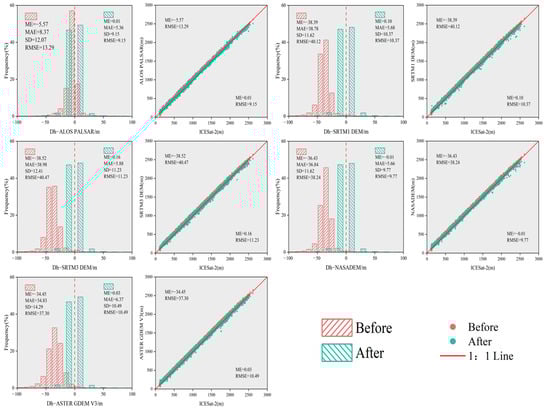
Figure 4.
ALOS PALSAR, SRTM1 DEM, SRTM3 DEM, NASADEM, and ASTER GDEM V3 elevation error histograms and scatter plots before and after the random forest model correction.
3.2. Comparison of the Accuracy of Five DEMs before and after Correction
3.2.1. DEM Accuracy Analysis before and after Correction Based on Slope
To comprehensively compare the accuracy and consistency of the five DEMs against different slope levels, precision analyses were conducted on the five DEMs before and after correction for different slope levels to observe the relationship between elevation differences and slope levels.
Before correction, we found that all DEMs exhibited negative biases and were in a significantly unstable state of dispersion. This means that under different slope levels, the DEM error distribution in Chongqing is inconsistent and there is a tendency for a large negative deviation from the true value. However, after applying random forest correction, we observed significant improvement. After correction, the error distributions of the five DEMs were symmetrically distributed around zero, indicating that the corrected DEMs more accurately reflected the terrain features of the various slope categories. Additionally, all DEMs showed uniformly distributed dispersion, resulting in more stable and consistent results, thereby largely eliminating negative biases. This result demonstrates the significant role of the random forest model in improving the accuracy and consistency of DEMs under different terrain conditions.
Table 3 presents the ME and RMSE of each DEM before and after correction for various slope levels, demonstrating a notable correlation between elevation accuracy and terrain slope. From Figure 5 and Table 3, it can be observed that as the slope level increases, the accuracy of each DEM exhibits a noticeable decrease both before and after correction. At the ≤5° level, SRTM3, NASA, and ASTER exhibit the highest accuracy, with cRMSE values of 3.74 m, 4.63 m, and 5.78 m, respectively. When the slope is greater than or equal to 20°, all DEM products exhibit the highest errors. Therefore, an increase in slope is positively correlated with a decrease in data accuracy, confirming the significant impact of terrain slope on DEM data quality.
Table 3.
Errors of the five DEMs before and after correction based on different slope grades.
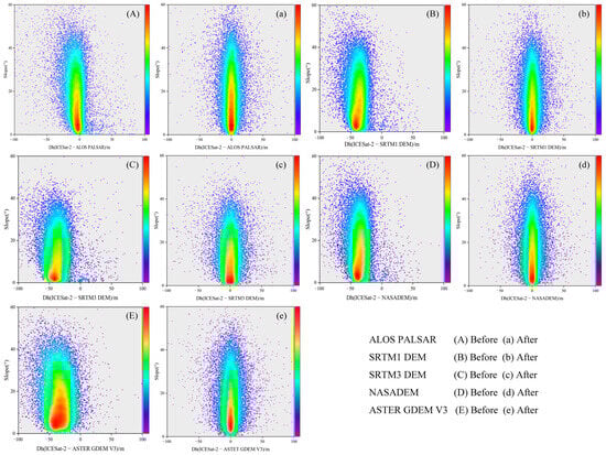
Figure 5.
Scatter density plots of the altimetric error before and after correction for ALOS PALSAR (A,a), SRTM1 DEM (B,b), SRTM3 DEM (C,c), NASADEM (D,d), and ASTER GDEM V3 (E,e) at different slopes.
3.2.2. DEM Accuracy Analysis before and after Correction Based on Aspect
Figure 6 depicts a radial radar chart illustrating the elevation errors of each DEM under different aspects. Before correction, all five DEMs exhibit noticeable errors in eight directions, with relatively consistent errors in each direction. Specifically, the error distribution range of the ALOS data is the smallest, ranging from 11.82 m to 14.47 m. The maximum error occurs in the due north direction, while the minimum error is in the due west direction. Similarly, the error distribution of the SRTM3 data is the largest, ranging from 39.66 m to 40.72 m, with the maximum errors occurring in the due east and southwest directions, and the minimum error in the northwest direction. The remaining three products are ranked in descending order of error as follows: ASTER, NASA, and SRTM1. Overall, before correction, the maximum error distributions of all DEMs are in the northeast and due east directions, while the minimum error distributions are in the northwest and due north directions.
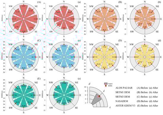
Figure 6.
Differences between five DEMs and ICESat-2 ATL08 depicted by radial radar plots for different slope directions before and after correction (red diamonds in the figure indicate RMSE): (A,a) ALOS PALSAR, (B,b) SRTM1 DEM, (C,c) SRTM3 DEM, (D,d) NASADEM, and (E,e) ASTER GDEM V3.
After correction, there were no significant differences in elevation errors among the five DEMs across the eight directions. The random forest model improved accuracy across all aspects. Among them, the smallest improvement was observed in the ALOS data, with the corrected cRMSE ranging from 8.71 m to 12.43 m. The maximum values occurred in the due north and southeast directions, while the minimum value occurred in the southwest direction. This may be because ALOS PALSAR itself has high data quality with a spatial resolution of 12.5 m, and already contains relatively accurate terrain information, hence the relatively small improvement after correction. In contrast, other digital elevation model products with lower spatial resolutions showed more significant improvements after correction. Additionally, the random forest model may not be suitable for correcting ALOS PALSAR data. Therefore, other correction methods or models, such as those based on deep learning or other nonlinear regression models, could be considered. SRTM1 showed the best correction effect, with a corrected cRMSE range of 8.50 m to 12.13 m. The maximum error occurred in the due north direction, while the minimum error occurred in the southeast direction. The other three DEMs were ranked in descending order of error as follows: NASA, ASTER, and SRTM3, with their maximum and minimum errors consistent with the former.
In summary, the random forest model improved the accuracy of the five DEM datasets in various aspects. Although no significant differences in elevation were observed across directions before and after correction, errors generally decreased after the correction.
3.2.3. DEM Accuracy Analysis before and after Correction Based on Land Cover Type
Figure 7 shows the elevation error distribution of five DEMs and ICESat-2 ATL08 in six land cover types, and uses histograms to statistically analyze the data before and after correction.
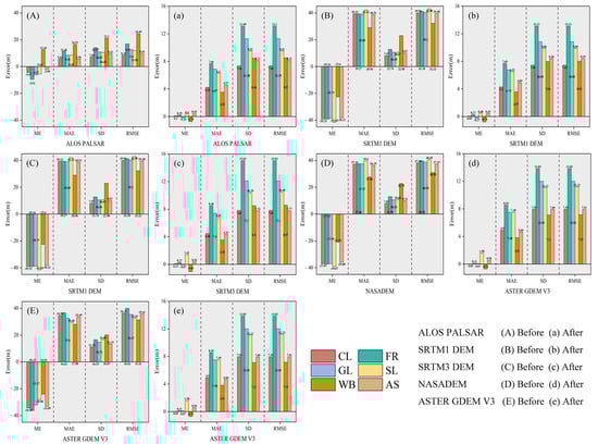
Figure 7.
Error histograms of ALOS PALSAR, SRTM1 DEM, SRTM3 DEM, NASADEM and ASTER GDEM V3 before and after correction under different land cover types. CL: cropland, FR: forest, GL: grassland, SL: shrubland, WB: water body, AS: artificial surface.
Before correction, ALOS data had the largest error in water bodies, with an RMSE of 24.49 m, while grassland had the smallest error, with an RMSE of 8.35 m. The minimum errors for the other four DEM products occurred in water bodies, except for ASTER, whose maximum error occurred in forests. The maximum values for the other three DEMs occurred in shrublands.
After correction, ALOS showed the most significant improvement for water bodies, with a decrease in cRMSE to 8.50m. Among them, NASA data showed the most significant improvement for forests, with a cRMSE of 12.94 m, while ASTER performed the least effectively for forests, with a cRMSE of 13.83 m. In terrain conditions with dense vegetation, the absorption and reflection effects of leaves, branches, and trunks cause the elevation information obtained by DEMs to fall within the vertical range of the vegetation rather than the actual land surface. Additionally, after correction, the minimum errors for ALOS and SRTM1 occurred in grassland types, with error proportions of 13%. The cRMSE values were 7.36 m and 7.45 m, respectively. The minimum errors for NASA and ASTER were observed in water bodies, with error proportions of 12% and cRMSE values of 6.39 m and 7.15 m, respectively. In contrast, the minimum error for SRTM3 shifted from water bodies to artificial surfaces, with an error proportion of 13% and a cRMSE of 7.77 m.
3.2.4. DEM Accuracy Analysis before and after Correction Based on Landform Types
Figure 8 illustrates the error distribution before and after correction for various terrain types. Due to the sparse sample points for the plain terrain type, it is not extensively described in this paper.
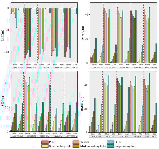
Figure 8.
Normal curve and axis whisker plots of error distribution of five DEMs before and after correction for different landform types.
By observing the visualized results, it is evident that all terrain types exhibited a significant decrease in all indicators before and after correction. All DEMs showed negative biases in the various types of terrain. After correction, the negative biases in all terrain types were significantly reduced. However, in the category of rugged mountains, negative biases still persisted even after correction, and the degree of bias was relatively significant. This complexity may be attributed to the rugged terrain in mountainous areas, which includes features such as cliffs and valleys. These features might have been misinterpreted or overlooked in the original data, leading to residual biases in the corrected data. Additionally, rugged mountainous terrain may be influenced by weather conditions such as cloud and fog, which could increase the uncertainty of the collected data and consequently affect accuracy.
Table 4 summarizes the ME and RMSE indicators of the five DEMs before and after correction. The minimum errors for all DEMs occurred in the plains, while the maximum errors were observed in the large rolling hills. Specifically, NASA performed the best in plains, terraces, and large rolling hills, with cRMSE values of 0.44 m, 2.67 m, and 23.31 m, respectively. However, ASTER performed the worst in plateaus and hills, with cRMSE values ranging from 3.25 m to 6.12 m. It is noteworthy that SRTM3 data exhibited the highest accuracy in terraces and hills. However, with increasing ruggedness, significant errors were observed, reaching a cRMSE of 38.41 m in rugged mountainous terrain. The cRMSE values for ALOS ranged from 2.84 m to 23.80 m. Compared to the other four DEM products, the correction effect of ALOS was consistent with the other terrain features. However, NASA exhibited better accuracy after correction compared to ALOS, with cRMSE values ranging from 2.67 m to 23.31 m. Following NASA, the order of performance was SRTM1, ASTER, and SRTM3, with cRMSE values ranging from 2.81 m to 24.23 m, 3.25 m to 24.62 m, and 2.77 m to 38.41 m, respectively.
Table 4.
Error of the five DEMs before and after correction based on landform types.
3.3. Global and Local Analysis of Five Types of DEM before and after Correction
Figure 9 shows the overall effects of the five DEMs before and after correction. To highlight the visual features of the five DEMs, we standardized their elevation ranges. No significant terrain variations were observed in the initial data. However, after correction with the random forest model, the terrain features of all global open-source DEMs were significantly improved. Especially in areas such as “Southwestern Chongqing” and “Northeast Chongqing”, the undulations of the terrain and the sense of vertical and horizontal terrain are more obvious. ALOS, NASA, and ASTER showed wide error ranges from −49 to 49. On the other hand, SRTM1 and SRTM3 had narrow error ranges, with variances of approximately ±1 m. Additionally, error distribution varied among the different DEMs. The error distributions of ALOS and NASA were relatively uniform, indicating consistent correction effects across different terrain conditions. However, ASTER’s error distribution was uneven, indicating potential limitations in the optical product’s data processing. Of SRTM1 and SRTM3, positive errors were more significant in SRTM1, while negative errors were more pronounced in SRTM3. This variation may result from the differences in data acquisition time and processing methods used in various DEM products. For example, SRTM data were released earlier, and may show slight terrain variations compared to other DEM products. In densely populated regions like “Southwest Chongqing,” human-induced changes may have caused variations in positive and negative errors between SRTM1 and SRTM3.
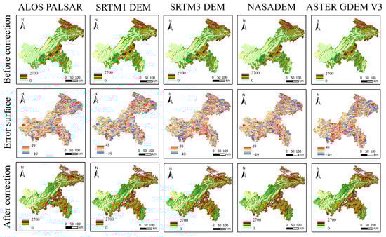
Figure 9.
Before and after comparison of five DEM corrections in Chongqing.
In our statistical analysis, we found that the maximum elevation recorded in the ALOS dataset was the lowest. According to a report from the Chongqing Forestry Bureau, the highest elevation in Chongqing is 2796.8 m (source: https://lyj.cq.gov.cn/, accessed on 4 May 2024). However, the highest elevation recorded in the ALOS dataset is 2700 m. This indicates that the elevation values in high-altitude areas in the ALOS dataset were underestimated before correction. After correction with the random forest model, a significant increase in the maximum elevation value was observed, reaching 2771 m. This finding further validates the effectiveness of the random forest model in improving the accuracy of DEMs. The corrected elevation values are now closer to the officially reported data, suggesting that the corrected data more accurately reflect geographical reality. These enhancements establish the groundwork for accurate terrain modeling in the Chongqing region, allowing for a more precise understanding and analysis of terrain features. This provides reliable geographic information support for urban planning, natural disaster prevention, and resource management.
Based on visual analysis, we extracted the local landform features of five different landform types within the study area. As shown in Figure 10, there were notable enhancements and adjustments in the globally available DEMs following correction. Particularly in areas with significant terrain variations, the corrected DEMs could more accurately depict mountainous terrain details. This included increasing terrain complexity, refining contour lines, and enhancing descriptions of terrain attributes. Through analyzing local features, we gained a better understanding of the impact of correcting DEM data. The corrected data showed improved performance across the different landform categories, highlighting the importance of these variations for terrain analysis and practical applications. The improvements provide more accurate terrain data, supporting research and decision making for urban planning in mountainous areas, resource management, and environmental planning. The corrected DEMs have improved accuracy and offer detailed terrain information, facilitating a better understanding and management of terrain features and environmental changes in mountainous regions.
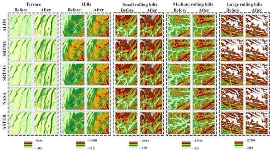
Figure 10.
Local features presented by the DEM data before and after the five corrections for different landforms.
4. Discussion
4.1. The Impact of Spatial Resolution on DEM Accuracy
We observed that the corrected RMSE values reflected the improvement in the accuracy of the individual DEM products. The ALOS data with a 12.5 m resolution showed a significant enhancement in precision. The RMSE values decreased from 13.29 m to 9.15 m after correction, indicating the notable effectiveness of the correction algorithm. In contrast, the 30 m resolution data from NASA and SRTM1 exhibited more significant improvements in accuracy post-correction, with RMSE values of 9.77 m and 10.37 m, respectively. These results may be closely related to the characteristics of the correction algorithm and the data source. The 90 m resolution SRTM3 data performed the poorest, with an RMSE of 11.23 m post-correction, highlighting the direct impact of spatial resolution on DEM accuracy. Higher spatial resolution enables a better representation of terrain details. Therefore, the ALOS product, with a 12.5 m resolution, maintained higher accuracy both pre- and post-correction, while the 90 m resolution SRTM3 exhibited the lowest overall accuracy. Further analysis revealed that different types of DEM products exhibit varying levels of accuracy at different spatial resolutions. This difference arises from the ability of higher spatial resolution to capture terrain details more effectively. It is worth noting that ALOS, SRTM, and NASA are all SAR products, while ASTER is an optical stereophotogrammetric product. Previous studies [57,58,59] have indicated that optical photogrammetric products inevitably produce shadows on images when observing the same area from different directions, resulting in void values and limited accuracy. Optical image capture and processing techniques are susceptible to weather and imaging conditions, such as cloud, fog, and sunlight. Therefore, lower accuracy is observed in the cloudy and foggy mountainous areas of Chongqing.
Furthermore, the random forest correction method not only enhanced the quality of the high-resolution DEM data, but also improved medium- and low-resolution DEM products, particularly in complex terrain areas [11,60,61]. Among them, the enhancement was most significant for NASA data, with the product being improved to meet practical application demands. Given the complex terrain of Chongqing, using suitable correction methods to improve DEM accuracy is crucial. These results highlight the significance of choosing suitable DEM products and correction methods for terrain modeling and related applications [62,63].
4.2. Slope and Aspect
Slope is one of the most important features of topography: it describes the degree of inclination of the ground surface relative to the horizontal axis and is a quantitative indicator of the steepness of terrain [32]. However, abrupt changes in slope can lead to discontinuities in surface elevation, making it challenging for sensors to accurately capture subtle terrain features during data collection and DEM generation [64].
Our results are consistent with previous studies [65,66] showing that the accuracy of DEMs exhibits significant uncertainty as slope class increases. This uncertainty may stem from two aspects. Firstly, the terrain in high-slope-class areas is usually steeper and more complex, resulting in sparser sample points, and this data imbalance may cause the model to favor terrain features with more sample points when learning, and the model may not be able to fully learn the complexity of terrain features, which affects the correction effect. Secondly, the random forest model may suffer from overfitting during the training process, resulting in poor extrapolation ability for terrain features with slopes >20°. This means that the model learns better for low-slope terrain in the training phase and performs poorly for high-slope terrain in the testing phase. These factors make it difficult for the model to accurately learn and predict terrain features in areas with higher slopes, which affects the effectiveness of the correction.
Additionally, we observed that aspect has a relatively minor impact on DEM accuracy. Although there was some improvement in accuracy in all aspects after correction, no significant features were observed in any aspect. This could be attributed to the random forest model showcasing consistent performance when handling aspect information, as it does not yield notable variances in accuracy among various aspects. These findings provide important insights into understanding the impact of terrain features on DEM accuracy and offer guidance for future improvements to correction methods and models.
4.3. Land Cover and Landform
Land-cover and terrain types exhibit distinct error features in DEMs, primarily due to the significant influence of vegetation cover. The reflection and scattering effects of vegetation can lead to fluctuations in remotely sensed signals, which can result in artifacts or blurring in DEMs, posing a challenge to the sensor in accurately detecting the ground [32,67]. This effect is particularly pronounced in areas with significant terrain variations. Shadow effects and vegetation obstruction make it more difficult to obtain accurate elevation information, thereby affecting the quality of the DEM.
Figure 9 and Figure 10 show notable changes in terrain features before and after correcting the DEM data. After correction, all DEM data show excellent performance in representing terrain features, especially in mountainous regions with significant elevation variations. However, there were noticeable differences in the surface errors of the SRTM1 and SRTM3 data compared to the other DEMs. This issue may arise from their earlier production times, leading to potential noise or data gaps during collection and processing. Despite using the latest released data and addressing noise and missing values, challenges may persist due to temporal differences and inadequate data processing techniques.
Among the correction methods we selected, the random forest algorithm effectively improved data accuracy and precision. However, even after correction, subtle errors or uncertainties may still exist due to limitations in the original data. Therefore, visualization may not effectively highlight subtle changes after correction, necessitating more sensitive visualization techniques or tools. To improve the accuracy of DEMs for different land-cover and terrain types, it is crucial to utilize advanced and adaptive algorithms for terrain features. In densely vegetated areas, adjustments to vegetation height can be made by integrating vegetation indices, vegetation height models, and leaf area indices to accurately estimate ground elevation. This approach helps reduce errors in elevation caused by vegetation. In addition, the accuracy of various land-cover types must be taken into account, along with the Bayesian average method [68] to merge different DEM data. These improvements are crucial for terrain analysis and practical applications in densely vegetated areas like Chongqing with complex landforms, and improve the credibility and accuracy of DEMs.
4.4. The Best DEM Choice for Mountainous Cities
Mountainous terrain is even more demanding on the accuracy of digital elevation models. Therefore, special attention is needed when selecting DEM data for applied research. Our results show that data with high spatial resolution are more suitable for application in studies that require higher data quality. For instance, the 12.5 m resolution ALOS data are better suited for extracting finer hydrological features and studying terrain in mountainous urban areas. However, considering issues related to data volume and storage, they may not be as suitable for extensive applications.
In contrast, the 30 m resolution SRTM1, NASA, and ASTER data are more suitable for comprehensive studies. Among them, NASA data exhibit higher robustness and are thus applicable to steep slopes and rugged terrain, and can rival higher-resolution data in describing terrain details. Secondly, SRTM1 data can be considered as an alternative.
However, it is not advisable to use the 30 m resolution ASTER data produced by optical photogrammetry techniques or the 90 m low-resolution SRTM3 data for mountainous urban areas. This is because mountainous urban terrain is complex, with shadow effects and dense vegetation cover posing challenges to the accuracy of optical products and low-resolution data [69,70,71]. It should be noted that although the accuracy of ASTER is higher than that of SRTM3, it is still not as good as high-resolution ALOS and high-quality NASA and SRTM1 data. In addition, ASTER and SRTM3 data have certain applicability in areas with simple terrain (plains, mesas, and hills), but they should be used with caution in mountainous cities with complex terrain.
4.5. Limitations and Recommendations
There are limitations to this work that must be acknowledged. Temporal inconsistencies in land-cover data can cause variability in results. The use of 2010 and 2020 data versions may not align with the production dates of the DEM data, potentially causing elevation changes, particularly in dynamic areas like water bodies and man-made surfaces. Therefore, the impact on the assessment results needs to be studied and analyzed in more depth. Secondly, this study did not consider the effect of factors such as the height and type of vegetation and seasonal changes in water bodies on topographic elevation. Future research could utilize high-precision vegetation data, such as global forest product and GEDI LiDAR data, in combination with long time series of water body area and water level height data, and incorporate these parameters into machine learning models to more comprehensively assess the accuracy and reliability of terrain data.
In addition, future research could explore the accuracy of other 30 m resolution optical and radar products in mountainous cities, like AW3D30 and COPERNICUS. The TanDEM-X product, a free 90 m LiDAR product, was recently released. However, further research is needed to assess its accuracy in representing terrain features in complex mountainous urban areas. Although open-source DEMs are globally accessible, variations in technical methods and collection timing result in differences in DEM quality. This necessitates the secondary verification of global DEM data, adding to the workload of other researchers.
In the future, it is important to consider researchers’ global DEM assessment results when producing DEMs. Especially in complex terrains like high-undulating mountains, glaciers, or karst terrain with broken features, it is essential to consider the impact of topographic factors. The application effects of new data products on terrain data should be explored to enhance research depth and accuracy.
5. Conclusions
This study conducted a comprehensive comparison and analysis of the accuracy of five DEMs using the case study of Chongqing. The aim was to evaluate their accuracy and applicability in mountainous urban environments. By analyzing the impact of terrain factors on DEM data quality and applying a random forest model for correction, we obtained some key findings.
- We found that spatial resolution is a major factor influencing the accuracy of DEMs. Data with higher spatial resolution, such as ALOS PALSAR, provide greater accuracy, especially in challenging terrains and dense vegetation areas. Additionally, we observed a positive correlation between slope and DEM accuracy. As the slope increases, the accuracy of the DEM generally decreases. The influence of aspect on DEM accuracy is relatively weak, but our correction method can improve the consistency of DEMs across various aspects.
- Vegetation cover and medium-to-large rolling hills pose significant challenges to the accuracy of DEMs. Before and after correction, all DEMs exhibited high error characteristics in vegetation types such as shrublands and forests. These factors are particularly important for complex mountainous urban terrain as they affect the quality and accuracy of DEM data.
- In mountainous urban areas like Chongqing, ALOS PALSAR and NASADEM demonstrate higher robustness and accuracy, especially after correction. Although the random forest model improved the accuracy of all DEMs, the correction effect was most significant for NASADEM, with its accuracy increasing by 74.44%. This was followed by SRTM1 DEM (74.15%), SRTM3 DEM (72.25%), ASTER GDEM V3 (71.12%), and ALOS PALSAR (31.15%). Therefore, selecting appropriate DEM datasets is crucial for research in mountainous urban areas. ALOS PALSAR and NASADEM outperformed the other datasets, mitigating the impact of terrain factors on DEM accuracy. This resulted in a more dependable and precise terrain data framework for research in mountainous urban areas.
In summary, these study results offer valuable insights for researching mountainous urban terrain and provide practical guidance on selecting DEM datasets and correction methods. Future research can explore new data products and correction methods to improve the accuracy and applicability of DEM data in complex terrain environments.
Author Contributions
Data curation, J.J., H.X. and D.W.; Formal analysis, W.X. and H.Y.; Methodology, W.X. and H.Y.; Resources, J.J., H.X. and D.W.; Supervision, J.L. and D.P.; Validation, W.X. and H.Y.; Visualization, J.L.; Writing—original draft, W.X.; Writing—review and editing, J.L. All authors have read and agreed to the published version of the manuscript.
Funding
This research was funded by Grant Program: National Key R&D Program, China; grant number 2019YFE0115200.
Data Availability Statement
The raw data supporting the conclusions of this article will be made available by the authors on request.
Conflicts of Interest
The authors declare no conflicts of interest.
References
- Berthier, E.; Arnaud, Y.; Kumar, R.; Ahmad, S.; Wagnon, P.; Chevallier, P. Remote sensing estimates of glacier mass balances in the Himachal Pradesh (Western Himalaya, India). Remote Sens. Environ. 2007, 108, 327–338. [Google Scholar] [CrossRef]
- Scown, M.W.; Thoms, M.C.; De Jager, N.R. Floodplain complexity and surface metrics: Influences of scale and geomorphology. Geomorphology 2015, 245, 102–116. [Google Scholar] [CrossRef]
- Courty, L.G.; Soriano-Monzalvo, J.C.; Pedrozo-Acuña, A. Evaluation of open-access global digital elevation models (AW3D30, SRTM, and ASTER) for flood modelling purposes. J. Flood Risk Manag. 2019, 12, e12550. [Google Scholar] [CrossRef]
- Natsagdorj, B.; Dalantai, S.; Sumiya, E.; Bao, Y.; Bayarsaikhan, S.; Batsaikhan, B.; Ganbat, D. Assessment of Some Meteorology Data of Average Monthly Air Temperature over Mongolia Using Digital Elevation Model (Dem) and Gis Techniques. Int. Arch. Photogramm. Remote Sens. Spat. Inf. Sci. 2021; 43, 117–121. [Google Scholar] [CrossRef]
- Elkhrachy, I. Vertical accuracy assessment for SRTM and ASTER Digital Elevation Models: A case study of Najran city, Saudi Arabia. Ain Shams Eng. J. 2018, 9, 1807–1817. [Google Scholar] [CrossRef]
- Sun, G.; Ranson, K.J.; Kharuk, V.I.; Kovacs, K. Validation of surface height from shuttle radar topography mission using shuttle laser altimeter. Remote Sens. Environ. 2003, 88, 401–411. [Google Scholar] [CrossRef]
- Peter, N.; Emmanuel, A.; Chukwuma, O. Determination of the Impacts of Landscape Offsets on the 30-metre SRTM DEM through a comparative analysis with Bare-Earth Elevations. In Proceedings of the FIG Working Week 2017, Helsinki, Finland, 29 May–2 June 2017. [Google Scholar]
- Greve, C. Digital Photogrammetry—An Addendum to the Manual of Photogrammetry; Publication of the American Society for Photogrammetry and Remote Sensing: Bethesda, MA, USA, 1996. [Google Scholar]
- Hanssen, R.F. Radar Interferometry: Data Interpretation and Error Analysis; Springer: New York, NY, USA, 2001. [Google Scholar]
- Lohr, U. Digital Elevation Models by Laser scanning. Photogramm. Rec. 1998, 16, 105–109. [Google Scholar] [CrossRef]
- Nitheshnirmal, S.; Thilagaraj, P.; Rahaman, S.A.; Jegankumar, R. Erosion risk assessment through morphometric indices for prioritisation of Arjuna watershed using ALOS-PALSAR DEM. Model. Earth Syst. Environ. 2019, 5, 907–924. [Google Scholar] [CrossRef]
- Farr, T.G.; Rosen, P.A.; Caro, E.; Crippen, R.; Duren, R.; Hensley, S.; Kobrick, M.; Paller, M.; Rodriguez, E.; Roth, L.; et al. The shuttle radar topography mission. Rev. Geophys. 2007, 45, 1–33. [Google Scholar] [CrossRef]
- Hirt, C.; Filmer, M.S.; Featherstone, W.E. Comparison and validation of the recent freely available ASTER-GDEM ver1, SRTM ver4.1 and GEODATA DEM-9S ver3 digital elevation models over Australia. Aust. J. Earth Sci. 2010, 57, 337–347. [Google Scholar] [CrossRef]
- Zink, M.; Bachmann, M.; Brautigam, B.; Fritz, T.; Hajnsek, I.; Moreira, A.; Wessel, B.; Krieger, G. TanDEM-X: The new global DEM takes shape. IEEE Geosci. Remote Sens. Mag. 2014, 2, 8–23. [Google Scholar] [CrossRef]
- Carter, J.R. Digital Representations of Topographic Surfaces. Photogramm. Eng. Remote Sens. 1988, 54, 1577–1580. [Google Scholar]
- Oksanen, J.; Sarjakoski, T. Error propagation of DEM-based surface derivatives. Comput. Geosci. 2005, 31, 1015–1027. [Google Scholar] [CrossRef]
- Cem, G.; Bedri, A.; Zeki, Y.Y.; Edip Müftüoğlu, A.; Güneysu, C.; Ertek, T.A.; Volkan, D.; Kaya, H. Morphologic Features of Kapıdağ Peninsula and its Coasts (NWTurkey) using by Remote Sensing and DTM. Int. J. Environ. Geoinformatics 2014, 1, 48–63. [Google Scholar] [CrossRef]
- KiliÇ, B.; GÜLgen, F.; ÇElen, M.; ÖNcel, S.; OruÇ, H.; Vural, S. Morphometric Analysis of Saz-Çayırova Drainage Basin using Geographic Information Systems and Different Digital Elevation Models. Int. J. Environ. Geoinformatics 2022, 9, 177–186. [Google Scholar] [CrossRef]
- Lakshmi, S.E.; Yarrakula, K. Review and critical analysis on digital elevation models. Geofizika 2019, 35, 129–157. [Google Scholar] [CrossRef]
- Athmania, D.; Achour, H. External Validation of the ASTER GDEM2, GMTED2010 and CGIAR-CSI- SRTM v4.1 Free Access Digital Elevation Models (DEMs) in Tunisia and Algeria. Remote Sens. 2014, 6, 4600–4620. [Google Scholar] [CrossRef]
- Fricker, H.A.; Borsa, A.; Minster, B.; Carabajal, C.; Quinn, K.; Bills, B. Assessment of ICESat performance at the salar de Uyuni, Bolivia. Geophys. Res. Lett. 2005, 32, L21S06. [Google Scholar] [CrossRef]
- Siegfried, M.R.; Hawley, R.L.; Burkhart, J.F. High-Resolution Ground-Based GPS Measurements Show Intercampaign Bias in ICESat Elevation Data Near Summit, Greenland. IEEE Trans. Geosci. Remote Sens. 2011, 49, 3393–3400. [Google Scholar] [CrossRef]
- Satgé, F.; Bonnet, M.P.; Timouk, F.; Calmant, S.; Pillco, R.; Molina, J.; Lavado-Casimiro, W.; Arsen, A.; Crétaux, J.F.; Garnier, J. Accuracy assessment of SRTM v4 and ASTER GDEM v2 over the Altiplano watershed using ICESat/GLAS data. Int. J. Remote Sens. 2015, 36, 465–488. [Google Scholar] [CrossRef]
- Gonzalez, J.H.; Bachmann, M.; Scheiber, R.; Krieger, G. Definition of ICESat Selection Criteria for Their Use as Height References for TanDEM-X. IEEE Trans. Geosci. Remote Sens. 2010, 48, 2750–2757. [Google Scholar] [CrossRef]
- Wang, C.; Zhu, X.; Nie, S.; Xi, X.; Li, D.; Zheng, W.; Chen, S. Ground elevation accuracy verification of ICESat-2 data: A case study in Alaska, USA. Opt. Express 2019, 27, 38168–38179. [Google Scholar] [CrossRef]
- Neuenschwander, A.L.; Magruder, L.A. Canopy and terrain height retrievals with ICESat-2: A first look. Remote Sens. 2019, 11, 1721. [Google Scholar] [CrossRef]
- Neuenschwander, A.; Guenther, E.; White, J.C.; Duncanson, L.; Montesano, P. Validation of ICESat-2 terrain and canopy heights in boreal forests. Remote Sens. Environ. 2020, 251, 112110. [Google Scholar] [CrossRef]
- Magruder, L.; Neuenschwander, A.; Klotz, B. Digital terrain model elevation corrections using space-based imagery and ICESat-2 laser altimetry. Remote Sens. Environ. 2021, 264, 112621. [Google Scholar] [CrossRef]
- Li, Y.; Fu, H.; Zhu, J.; Wu, K.; Yang, P.; Wang, L.; Gao, S. A method for SRTM DEM elevation error correction in forested areas using ICESat-2 data and vegetation classification data. Remote Sens. 2022, 14, 3380. [Google Scholar] [CrossRef]
- Xu, W.; Li, J.; Peng, D.; Jiang, J.; Xia, H.; Yin, H.; Yang, J. Multi-source DEM accuracy evaluation based on ICESat-2 in Qinghai-Tibet Plateau, China. Int. J. Digit. Earth 2023, 17, 2297843. [Google Scholar] [CrossRef]
- Ernesto, R.; Charles, S.M.; Eric, B.J. A Global Assessment of the SRTM Performance. Photogramm. Eng. Remote Sens. 2006, 72, 249–260. [Google Scholar] [CrossRef]
- Varga, M.; Bašić, T. Accuracy validation and comparison of global digital elevation models over Croatia. Int. J. Remote Sens. 2015, 36, 170–189. [Google Scholar] [CrossRef]
- Yap, L.; Kandé, L.H.; Nouayou, R.; Kamguia, J.; Ngouh, N.A.; Makuate, M.B. Vertical accuracy evaluation of freely available latest high-resolution (30 m) global digital elevation models over Cameroon (Central Africa) with GPS/leveling ground control points. Int. J. Digit. Earth 2018, 12, 500–524. [Google Scholar] [CrossRef]
- Chen, C.; Yang, S.; Li, Y. Accuracy assessment and correction of SRTM DEM using ICESat/GLAS data under data coregistration. Remote Sens. 2020, 12, 3435. [Google Scholar] [CrossRef]
- Du, P.; Bai, X.; Tan, K.; Xue, Z.; Samat, A.; Xia, J.; Li, E.; Su, H.; Liu, W. Advances of Four Machine Learning Methods for Spatial Data Handling: A Review. J. Geovisualization Spat. Anal. 2020, 4, 13. [Google Scholar] [CrossRef]
- Zhao, S.; Liu, J.; Cheng, W.; Zhou, C. Fusion Scheme and Implementation Based on SRTM1, ASTER GDEM V3, and AW3D30. ISPRS Int. J. Geo-Inf. 2022, 11, 207. [Google Scholar] [CrossRef]
- Crippen, R.; Buckley, S.; Agram, P.; Belz, E.; Gurrola, E.; Hensley, S.; Kobrick, M.; Lavalle, M.; Martin, J.; Neumann, M.; et al. Nasadem Global Elevation Model: Methods and Progress. ISPRS-Int. Arch. Photogramm. Remote Sens. Spat. Inf. Sci. 2016; 41, 125–128. [Google Scholar] [CrossRef]
- Buckley, S.M.; Agram, P.S.; Belz, J.E.; Crippen, R.E.; Gurrola, E.M.; Hensley, S.; Kobrick, M.; Lavalle, M.; Martin, J.M.; Neumann, M.; et al. NASA DEM: User Guide (Technical Report January). 2020. Available online: https://lpdaac.usgs.gov/documents/592/NASADEM_User_Guide_V1.pdf (accessed on 4 May 2024).
- Li, H.; Zhao, J.; Yan, B.; Yue, L.; Wang, L. Global DEMs vary from one to another: An evaluation of newly released Copernicus, NASA and AW3D30 DEM on selected terrains of China using ICESat-2 altimetry data. Int. J. Digit. Earth 2022, 15, 1149–1168. [Google Scholar] [CrossRef]
- Gesch, D.; Oimoen, M.; Danielson, J.; Meyer, D. Validation of the Aster Global Digital Elevation Model Version 3 over the Conterminous United States. ISPRS-Int. Arch. Photogramm. Remote Sens. Spat. Inf. Sci. 2016; 41, 143–148. [Google Scholar] [CrossRef]
- Markus, T.; Neumann, T.; Martino, A.; Abdalati, W.; Brunt, K.; Csatho, B.; Farrell, S.; Fricker, H.; Gardner, A.; Harding, D.; et al. The ice, cloud, and land elevation satellite-2 (ICESat-2): Science requirements, concept, and implementation. Remote Sens. Environ. 2017, 190, 260–273. [Google Scholar] [CrossRef]
- Neumann, T.A.; Martino, A.J.; Markus, T.; Bae, S.; Bock, M.R.; Brenner, A.C.; Brunt, K.M.; Cavanaugh, J.; Fernandes, S.T.; Hancock, D.W.; et al. The ice, cloud, and land elevation satellite—2 mission: A global geolocated photon product derived from the advanced topographic laser altimeter system. Remote Sens. Environ. 2019, 233, 111325. [Google Scholar] [CrossRef]
- Neuenschwander, A.; Pitts, K. The ATL08 land and vegetation product for the ICESat-2 Mission. Remote Sens. Environ. 2019, 221, 247–259. [Google Scholar] [CrossRef]
- Amy Neuenschwander, K.P.; Jelley, B.; Robbins, J. Ice, Cloud, and Land Elevation Satellite-2 (ICESat-2) Algorithm Theoretical Basis Document (ATBD); icesat2_atl08_atbd_r005_1; NASA: Greenbelt, MA, USA, 2022; Volume 2, p. 2022. [Google Scholar]
- Liu, A.; Cheng, X.; Chen, Z. Performance evaluation of GEDI and ICESat-2 laser altimeter data for terrain and canopy height retrievals. Remote Sens. Environ. 2021, 264, 112571. [Google Scholar] [CrossRef]
- Osama, N.; Shao, Z.; Ma, Y.; Yan, J.; Fan, Y.; Magdy Habib, S.; Freeshah, M. The ATL08 as a height reference for the global digital elevation models. Geo-Spat. Inf. Sci. 2022, 27, 327–346. [Google Scholar] [CrossRef]
- Li, B.; Xie, H.; Tong, X.; Liu, S.; Xu, Q.; Sun, Y. Extracting accurate terrain in vegetated areas from ICESat-2 data. International J. Appl. Earth Obs. Geoinf. 2023, 117, 103200. [Google Scholar] [CrossRef]
- Atmani, F.; Bookhagen, B.; Smith, T. Measuring Vegetation Heights and Their Seasonal Changes in the Western Namibian Savanna Using Spaceborne Lidars. Remote Sens. 2022, 14, 2928. [Google Scholar] [CrossRef]
- Shang, D.; Zhang, Y.; Dai, C.; Ma, Q.; Wang, Z. Extraction Strategy for ICESat-2 Elevation Control Points Based on ATL08 Product. IEEE Trans. Geosci. Remote Sens. 2022, 60, 5705012. [Google Scholar] [CrossRef]
- del Rosario González-Moradas, M.; Viveen, W. Evaluation of ASTER GDEM2, SRTMv3.0, ALOS AW3D30 and TanDEM-X DEMs for the Peruvian Andes against highly accurate GNSS ground control points and geomorphological-hydrological metrics. Remote Sens. Environ. 2020, 237, 111509. [Google Scholar] [CrossRef]
- Yamazaki, D.; Ikeshima, D.; Sosa, J.; Bates, P.D.; Allen, G.H.; Pavelsky, T.M. MERIT Hydro: A High-Resolution Global Hydrography Map Based on Latest Topography Dataset. Water Resour. Res. 2019, 55, 5053–5073. [Google Scholar] [CrossRef]
- Nardi, F.; Annis, A.; Di Baldassarre, G.; Vivoni, E.R.; Grimaldi, S. GFPLAIN250m, a global high-resolution dataset of Earth’s floodplains. Sci. Data 2019, 6, 180309. [Google Scholar] [CrossRef] [PubMed]
- Breiman, L. Random Forests. Mach. Learn. 2001, 45, 5–32. [Google Scholar] [CrossRef]
- He, X.; Chaney, N.W.; Schleiss, M.; Sheffield, J. Spatial downscaling of precipitation using adaptable random forests. Water Resour. Res. 2016, 52, 8217–8237. [Google Scholar] [CrossRef]
- Su, Y.; Guo, Q. A practical method for SRTM DEM correction over vegetated mountain areas. ISPRS J. Photogramm. Remote Sens. 2014, 87, 216–228. [Google Scholar] [CrossRef]
- Hu, M.; Ji, S. Accuracy evaluation and improvement of common DEM in Hubei Region based on ICESat/GLAS data. Earth Sci. Inform. 2021, 15, 221–231. [Google Scholar] [CrossRef]
- Li, H.; Deng, Q.; Wang, L. Automatic co-registration of digital elevation models based on centroids of subwatersheds. IEEE Trans. Geosci. Remote Sens. 2017, 55, 6639–6650. [Google Scholar] [CrossRef]
- Liu, X.; Ran, M.; Xia, H.; Deng, M. Evaluating Vertical Accuracies of Open-Source Digital Elevation Models over Multiple Sites in China Using GPS Control Points. Remote Sens. 2022, 14, 2000. [Google Scholar] [CrossRef]
- Huang, J.; Wei, L.; Chen, T.; Luo, M.; Yang, H.; Sang, Y. Evaluation of DEM Accuracy Improvement Methods Based on Multi-Source Data Fusion in Typical Gully Areas of Loess Plateau. Sensors 2023, 23, 3878. [Google Scholar] [CrossRef] [PubMed]
- Das, A.; Agrawal, R.; Mohan, S. Topographic correction of ALOS-PALSAR images using InSAR-derived DEM. Geocarto Int. 2014, 30, 145–153. [Google Scholar] [CrossRef]
- Mesa-Mingorance, J.L.; Ariza-López, F.J. Accuracy Assessment of Digital Elevation Models (DEMs): A Critical Review of Practices of the Past Three Decades. Remote Sens. 2020, 12, 2630. [Google Scholar] [CrossRef]
- Ouyang, Z.; Zhou, C.; Xie, J.; Zhu, J.; Zhang, G.; Ao, M. SRTM DEM correction using ensemble machine learning algorithm. Remote Sens. 2023, 15, 3946. [Google Scholar] [CrossRef]
- Meadows, M.; Wilson, M. A Comparison of Machine Learning Approaches to Improve Free Topography Data for Flood Modelling. Remote Sens. 2021, 13, 275. [Google Scholar] [CrossRef]
- Li, H.; Zhao, J. Evaluation of the newly released worldwide AW3D30 DEM over typical landforms of China using two global DEMs and ICESat/GLAS data. IEEE J. Sel. Top. Appl. Earth Obs. Remote Sens. 2018, 11, 4430–4440. [Google Scholar] [CrossRef]
- Uuemaa, E.; Ahi, S.; Montibeller, B.; Muru, M.; Kmoch, A. Vertical accuracy of freely available global digital elevation models (ASTER, AW3D30, MERIT, TanDEM-X, SRTM, and NASADEM). Remote Sens. 2020, 12, 3482. [Google Scholar] [CrossRef]
- Li, M.; Yin, X.; Tang, B.-H.; Yang, M. Accuracy Assessment of High-Resolution Globally Available Open-Source DEMs Using ICESat/GLAS over Mountainous Areas, A Case Study in Yunnan Province, China. Remote Sens. 2023, 15, 1952. [Google Scholar] [CrossRef]
- Zhao, X.; Su, Y.; Hu, T.; Chen, L.; Gao, S.; Wang, R.; Jin, S.; Guo, Q. A global corrected SRTM DEM product for vegetated areas. Remote Sens. Lett. 2018, 9, 393–402. [Google Scholar] [CrossRef]
- Zhou, C.; Zhang, G.; Yang, Z.; Ao, M.; Liu, Z.; Zhu, J. An adaptive terrain-dependent method for SRTM DEM correction over mountainous areas. IEEE Access 2020, 8, 130878–130887. [Google Scholar] [CrossRef]
- Pham, H.T.; Marshall, L.; Johnson, F.; Sharma, A. A method for combining SRTM DEM and ASTER GDEM2 to improve topography estimation in regions without reference data. Remote Sens. Environ. 2018, 210, 229–241. [Google Scholar] [CrossRef]
- Guan, L.; Pan, H.; Zou, S.; Hu, J.; Zhu, X.; Zhou, P. The impact of horizontal errors on the accuracy of freely available Digital Elevation Models (DEMs). Int. J. Remote Sens. 2020, 41, 7383–7399. [Google Scholar] [CrossRef]
- Shen, X.; Zhou, C.; Zhu, J. Improving the Accuracy of TanDEM-X Digital Elevation Model Using Least Squares Collocation Method. Remote Sens. 2023, 15, 3695. [Google Scholar] [CrossRef]
Disclaimer/Publisher’s Note: The statements, opinions and data contained in all publications are solely those of the individual author(s) and contributor(s) and not of MDPI and/or the editor(s). MDPI and/or the editor(s) disclaim responsibility for any injury to people or property resulting from any ideas, methods, instructions or products referred to in the content. |
© 2024 by the authors. Licensee MDPI, Basel, Switzerland. This article is an open access article distributed under the terms and conditions of the Creative Commons Attribution (CC BY) license (https://creativecommons.org/licenses/by/4.0/).