Article

Validation of Red-Edge Vegetation Indices in Vegetation Classification in Tropical Monsoon Region—A Case Study in Wenchang, Hainan, China

1
Key Laboratory of Earth Observation of Hainan Province, Hainan Aerospace Information Research Institute, Wenchang 571300, China
2
Aerospace Information Research Institute, Chinese Academy of Sciences, Beijing 100094, China
3
College of Civil Engineering, Henan University of Engineering, Zhengzhou 451191, China
4
North China Institute of Aerospace Industry, Langfang 065000, China
5
School of Geography and Remote Sensing, Guangzhou University, Guangzhou 510006, China
*
Author to whom correspondence should be addressed.
Remote Sens. 2024, 16(11), 1865; https://doi.org/10.3390/rs16111865
Submission received: 31 March 2024 / Revised: 20 May 2024 / Accepted: 21 May 2024 / Published: 23 May 2024

Abstract

:
Vegetation classification has always been the focus of remote sensing applications, especially for tropical regions with fragmented terrain, cloudy and rainy climates, and dense vegetation. How to effectively classify vegetation in tropical regions by using multi-spectral remote sensing with high resolution and red-edge spectrum needs to be further verified. Based on the experiment in Wenchang, Hainan, China, which is located in the tropical monsoon region, and combined with the ZY-1 02D 2.5 m fused images in January, March, July, and August, this paper discusses whether NDVI and four red-edge vegetation indices (VIs), CIre, NDVIre, MCARI, and TCARI, can promote vegetation classification and reduce the saturation. The results show that the schemes with the highest classification accuracies in all phases are those in which the red-edge VIs are involved, which suggests that the red-edge VIs can effectively contribute to the classification of vegetation. The maximum accuracy of the single phase is 86%, and the combined accuracy of the four phases can be improved to 92%. It has also been found that CIre and NDVIre do not reach saturation as easily as NDVI and MCARI in July and August, and their ability to enhance the separability between different vegetation types is superior to that of TCARI. In general, red-edge VIs can effectively promote vegetation classification in tropical monsoon regions, and red-edge VIs, such as CIre and NDVIre, have an anti-saturation performance, which can slow down the confusion between different vegetation types due to saturation.

1. Introduction

Vegetation resources are the material bases for human survival, including crops, woodlands, grasslands, and other categories, which provide important ecosystem services for human production and life. Adequate monitoring of vegetation resources is therefore an important prerequisite for assisting decision-making and tracking management. Multi-spectral remote sensing technology has become an effective means of monitoring vegetation resources because of its advantages such as rich data resources, wide coverage and fast timeliness. Multi-spectral remote sensing has been fully utilized in vegetation classification with the help of various types of remote sensing features, but the number of types that can be distinguished and the accuracy of classification still need to be improved. Especially in the tropical monsoon region, where the terrain is fragmented, the weather is cloudy and rainy, and the vegetation is dense, the uncertainty of remote sensing observation has been enhanced, and the complexity of vegetation classification has been greatly increased [1,2]. The tropical monsoon climate is distributed in most parts of South Asia and Southeast Asia from 10°N to the Tropic of Cancer, such as Southern Taiwan Province, Leizhou Peninsula of Guangdong Province, Hainan Province and Southern Yunnan Province of China, Indochina Peninsula, most of the Indian Peninsula, Philippines and other places. It is of great significance to strengthen the research on vegetation classification in the tropical monsoon region.
VIs as an indicator that can reflect the growth and coverage of vegetation, are widely used in land cover classification, inversion of vegetation physiological and ecological parameters, vegetation type identification, and so on. Among them, the Normalized Difference Vegetation Index (NDVI) is the most widely used [3,4]. NDVI can clearly differentiate green vegetation from the soil background with long-term observation availability and ease of use. However, the vegetation in tropical monsoon regions is generally dense. Due to the saturation of the red light channel and the inherent saturation defect of its formula, NDVI is prone to saturation in areas with high vegetation coverage, resulting in decreased sensitivity to dense vegetation and reduced vegetation identification efficiency [5,6]. Based on Difference Vegetation Index (DVI), Enhanced Vegetation Index (EVI), Green Normalized Difference Vegetation Index (GNDVI), NDVI, Ratio Vegetation Index (RVI), Soil Adjusted Vegetation Index (SAVI) and other VIs, by using the images of Sentinel, Landsat and the standard vegetation products of MODIS, SPOT4, scholars have carried out some studies on vegetation classification in tropical monsoon climate regions [7,8,9,10,11,12,13,14]. However, most of these studies are based on middle- and low-resolution images, and adopt VIs based on visible, near-infrared, and short-wave infrared. There are few studies on the effectiveness of red edge and its vegetation index, which are closely related to the pigmentation status of vegetation.
The red edge is closely related to the physicochemical parameters of green vegetation and can change with vegetation species and growth stage. Red-edge information was first applied in hyperspectral remote sensing and is commonly used in the inversion of vegetation physiological and biochemical parameters such as chlorophyll content, Leaf Area Index (LAI), biomass, nitrogen content, as well as in the monitoring of crop growth and pests [15]. Previous studies have shown that the red-edge VIs are more sensitive to plant physiological conditions than NDVI, and have certain anti-saturation performance [16,17]. For example, compared with NDVI, Delegido et al. obtained the strongest linear correlation between red-edge normalized difference index (NDI) and LAI in combination with 674 nm and 712 nm bands, and NDI was not saturated at a large value [18]. At present, more and more multispectral satellites have increased the red-edge spectrum, such as RapidEye, WorldView-2/3, Sentinel-2, and China’s GF-6 and ZY1-02D/E satellites. A few studies have shown that the red-edge VIs can enhance the separability for vegetation classification and identification. Üstüner et al. explored the effects of NDVI, GNDVI, and Normalized Difference Red-Edge Index (NDRE) on crop classification in the Aegean region based on the RapidEye images, and found that the NDRE contributed the most to the classification accuracy [19]. Wu Jing et al., conducted a fine classification of crops in Jingtai County based on Sentinel-2A data, confirming that the Red-Edge Normalized Vegetation Index (RENDVI) can assist NDVI in improving the classification accuracy [20]. Huang et al. classified the plantation types of Gaofeng Forest Farm in Guangxi based on the GF-6 WFV image, and the classification accuracy was the highest by using the combination of 8-band, Chlorophyll Index red edge (CIre) and New Inverted Red Edge Chlorophyll Index (IRECI) [21]. However, these classifications mainly explore the vegetation classification performance of the red-edge VIs. Few studies have been conducted on the effectiveness and anti-saturation properties of red-edge VIs in vegetation classification in tropical monsoon areas.
The saturation condition of NDVI will change with the growth stages of different vegetation types, that is, the saturation characteristics of NDVI have phenological changes. Time series VIs can reflect the growth process and phenological characteristics of different vegetation types, and it is a commonly used method in existing research. Yan et al. extracted the phenological characteristics of vegetation on the basis of constructing the time series NDVI and EVI and realized the high-precision classification of eight vegetation types. The result shows that adding phenological characteristics to the time series VIs is helpful to further improve the classification accuracy [22]. Combined with the time series red-edge VIs, related application research has also been carried out in a small amount. Zheng et al., constructed time series CIre and NDVI based on the ground spectrum to detect the main phenological phases of rice [23]. The result shows that CIre can accurately estimate the jointing, booting, and graining stages of rice and combined with CIre and NDVI can effectively serve the management of irrigation, fertilization, and harvest.
This paper takes Wenchang, Hainan, China as the study area, which is located in the tropical monsoon region and uses multi-temporal ZY1-02D visible near-infrared (VNIR) sensor images as the data source. The main research objectives are: (1) to make full use of the red-edge VIs of multi-temporal images to realize high-precision vegetation classification of fragmented terrain; (2) to explore whether the red-edge VIs are sensitive to the tropical vegetation types and whether they can solve the saturation problem of NDVI in the vegetation classification, so as to promote the effective application of the red-edge VIs.

2. Materials and Methods

2.1. Study Area and Data Sources

2.1.1. Overview of the Study Area and Field Survey

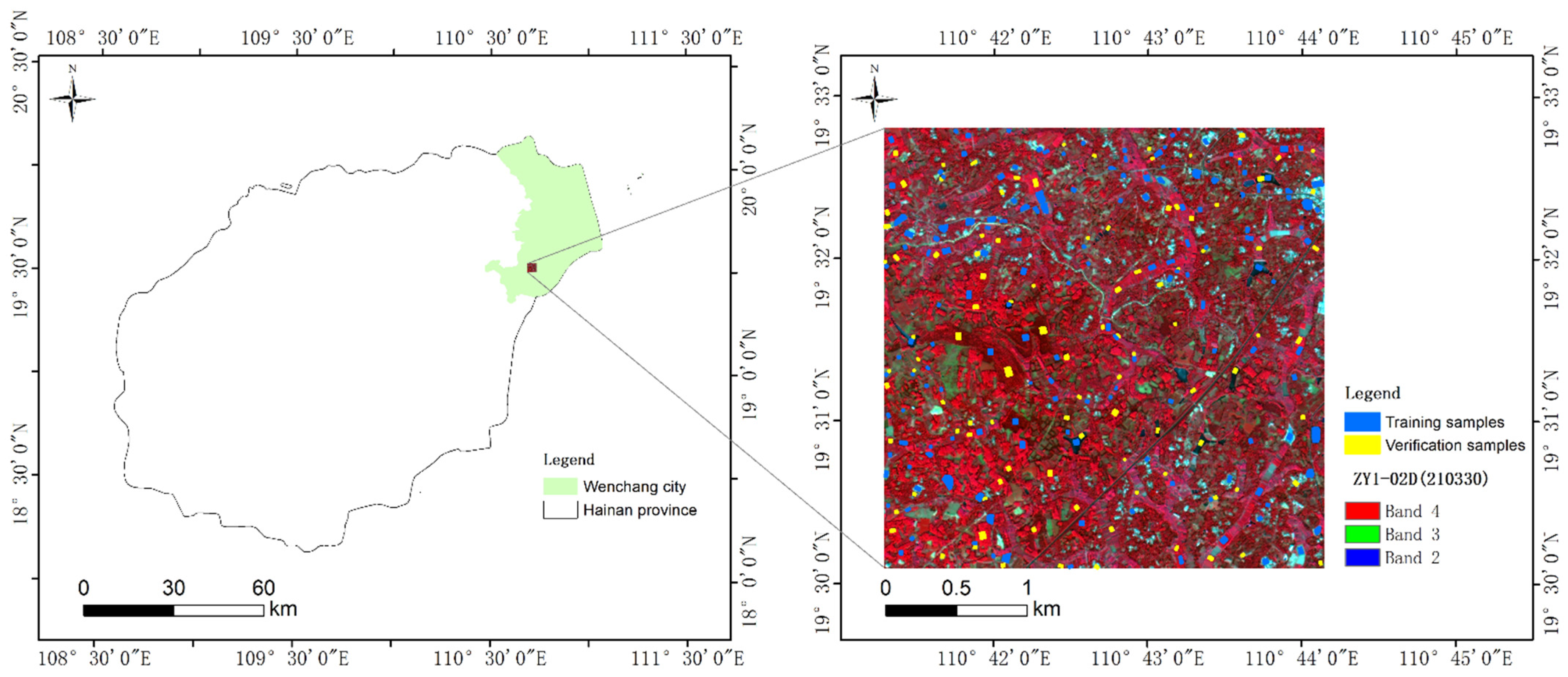
The study area is located in Wenchang City, Hainan Province, China (Figure 1). The geographic coordinates of Wenchang lie between 19°21′–20°1′N latitude and 110°28′–111°03′E longitude. The terrain is a low-hill plain with flat terrain in the northeast and undulating terrain in the southwest. Wenchang City is a tropical monsoon marine climate, characterized by abundant rainfall and sunshine, and is frost-free all year round. The four seasons are not distinct, which is reflected in the absence of hot summer and cold winter, and the annual temperature difference is small, with an annual average temperature of 24.4 °C, the average temperature of the coldest month is 18.5 °C, and that of the hottest month is 28.5 °C. Wenchang has obvious dry and rainy seasons, among which winter and spring are dry, summer and autumn are rainy, and the rainy season is mainly concentrated from May to October, accounting for 79% of the annual precipitation. Wenchang is rich in vegetation types, mainly including rubber, coconut, mangrove, mixed secondary forest, tropical fruit trees, pepper, and short scrub sparse grass, etc. Crops mainly include rice, vegetables, and melon fruits.
From 23 to 25 March 2021, a field survey was conducted in the central part of Wenchang City in an area of about 20 km × 20 km. At this time, early rice is in the booting and heading stage, winter melons and vegetables are in the maturity stage, and tropical fruits are in the small fruit expansion stage. Samples of forest, cultivated land, garden, water area, impervious surface, and other cover types were collected by the hand-held Global Navigation Satellite System (GNSS) receiver (Haida Zhong, Guangzhou, China), and photographs were taken. The survey routes covered most of the vegetation types with a relatively even distribution. A total of 459 valid sample points and 415 valid polygonal samples were obtained in this survey, which can provide a sample data base for the vegetation classification.

2.1.2. Remote Sensing Images

In view of the fact that the study area requires high resolution of images due to the fragmented terrain, multi-temporal ZY1-02D VNIR sensor images were used as the data source.
ZY1-02D satellite, an important model in China’s space infrastructure planning, was launched on 12 September 2019 and is China’s first civil hyperspectral operational satellite, carrying a 9-band VNIR camera and a 166-band hyperspectral camera, providing 2.5 m panchromatic, 10 m multispectral and 30 m hyperspectral image data. The VNIR camera’s Pan and B1~B4 (R, G, B, and NIR) spectral bands are the five most widely used spectral band configurations at home and abroad. The configuration of these spectral bands is the same as that of general remote sensing satellites, which is convenient for data fusion and image comparison. The configuration of B5~B8 spectral bands is the same as that of the new spectral bands of WordView-2, of which B7 spectral band is a red-edge spectral band. These spectral bands have important applications in resource distribution, soil water monitoring, atmospheric composition analysis, crop yield estimation, and so on. The main parameter information of ZY1-02D VNIR camera is shown in Table 1.
All available time series images of ZY1-02D VNIR camera in the field survey area in 2021 have been collected, covering four phases of January, March, July, and August, which are 2 January, 30 March, 24 July, and 19 August, 2021, respectively. The images of 30 March and 19 August are nearly cloudless and of good quality, and 30 March coincides with the time of the field survey. But there are a large number of cloud-covered areas in the images on 2 January and 24 July, obscuring part of the field survey area. In this study, ENVI processing software (version 5.3.1) was used to preprocess the ZY1-02D VNIR image by atmospheric correction, image fusion, and image registration. The FLAASH atmospheric correction module was applied to obtain the surface reflectance data [24,25]. The multispectral and panchromatic images were fused by the Gram–Schmidt procedure to produce the pan-sharpened multispectral images [26]. The geometric registration was carried out with reference to the 1.2 m Google Earth image by controlling the accuracy of less than 1 pixel. The fused and registered 2.5 m resolution surface reflectance products were obtained, so as to facilitate the subsequent calculation and application of VIs.

2.1.3. Sample Data

Due to the serious cloud coverage of the ZY1-02D images on 20 January and 24 July 2021, in order to make full use of the four time series images, a 5 km × 5 km nearly cloud-free area was selected as the study area in the 20 km × 20 km field survey area. The study area is a gently sloping terrace, and the vegetation types mainly contain tropical forest fruits such as lychee and pineapple, coconut groves, rubber, rice, pepper, etc., which are characterized by diverse landscape types and high degree of fragmentation. The vegetation types in the study area are divided into woodland, garden, paddy field, and dry land. Among them, the woodland includes coconut forest, rubber forest, miscellaneous wood secondary forest, etc. The gardens are mainly tropical fruit and pepper gardens. Dry land mainly includes vegetables, melon fruits, peanuts, and corn. Combined with the four time series images, Wenchang is in the dry season in January and March, and the leaves of coconut trees and other woodlands grow slowly, and fewer new leaves are extracted. In July and August, the woodlands grow rapidly. In gardens such as lychee, shoot branching controlling is carried out in January and March to promote flowering, with vigorous summer and autumn branch growth in July and August. Early rice is booted in March, harvested successively in July and August, followed by late rice, and harvested before the end of the year. Vegetables, melon fruits, and other crops on dry land can be grown all year round.
Combined with field survey samples and manual interpretation of high-resolution Google Earth images, a total of 256 polygon samples are marked (Figure 1). A total of 60% of the samples are randomly selected as training samples and the rest as verification samples, which are used for vegetation classification and subsequent precision verification. The number of polygons for training and verification and their corresponding pixel numbers are shown in Table 2.

2.2. Research Method

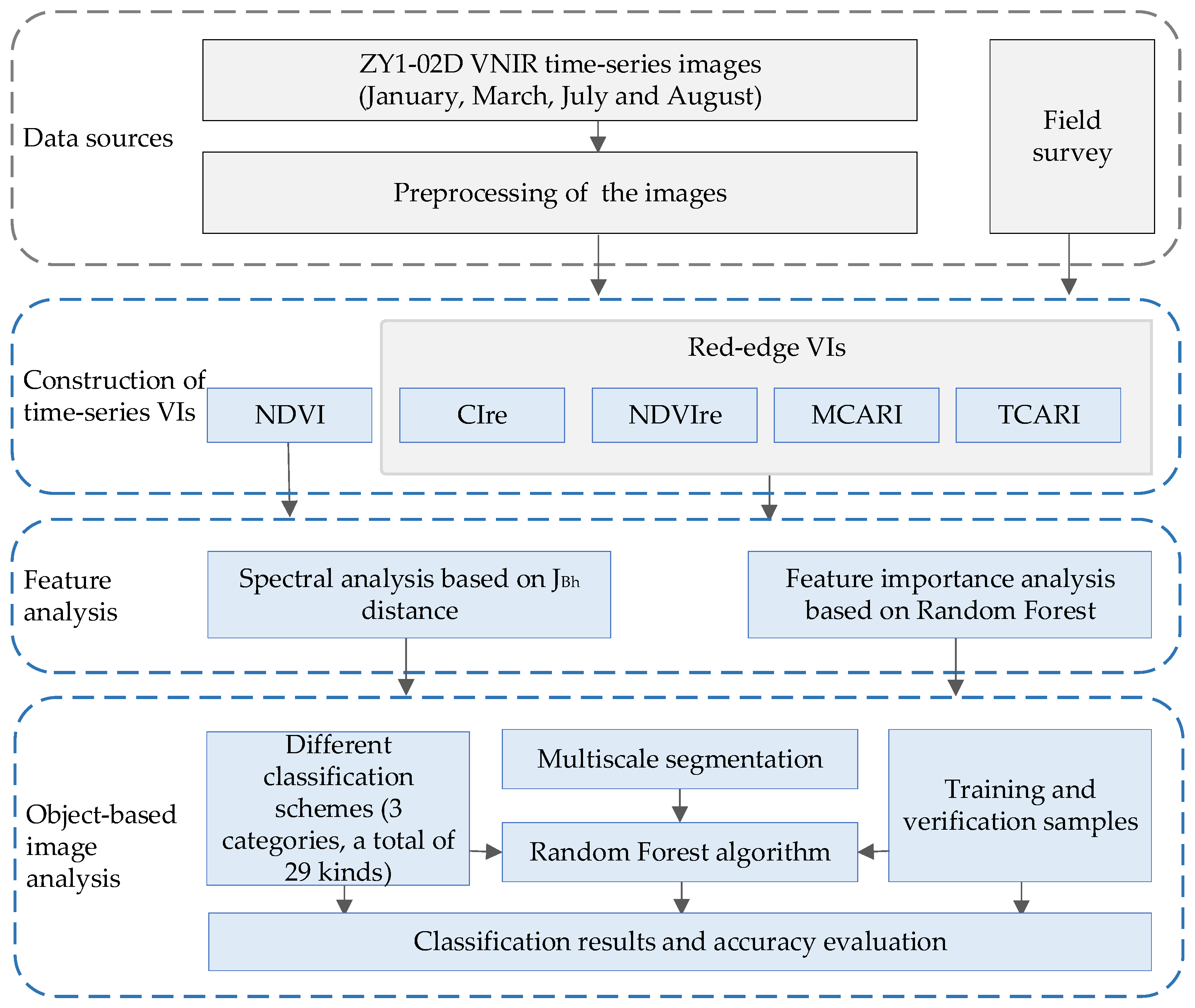
In this study, five VIs are constructed by taking advantage of the ZY1-02D VNIR imagery with the red-edge band and using the four time series imagery in January, March, July, and August 2021. Firstly, the spectral characterization of the red-edge bands for inter-class separability is carried out by using the JBh distance. Subsequently, the importance of different spectra and VIs for the four time series images is evaluated by using the Random Forest (RF) feature selection method. Finally, different classification schemes are designed, and vegetation types are classified by using object-based image analysis (OBIA) method, and the anti-saturation performance of different VIs is analyzed. The technical route of the study is shown in Figure 2.

2.2.1. Dataset Construction of Red-Edge Time Series VIs

Combined with the characteristics of ZY1-02D VNIR image with red-edge band, five VIs are constructed in this paper, including NDVI and four red-edge VIs, and the calculation formulas are shown in Table 3. The VIs of different time series imagery are obtained by band math.

2.2.2. Feature Analysis Method

  • Spectral feature analysis
The classification of remote-sensing images mainly uses the spectral features of the image and uses JBh distance method based on inter-class separability to analyze the spectral features of ZY1-02D VNIR image.
The performance of classifier depends largely on whether features can accurately describe the nature of objects, so separability criteria such as J-M distance are needed to measure the separability between various features. J-M distance can well reflect the actual relationship with classification accuracy, but it can only measure the separability between every two kinds and has the defect that it cannot reflect the separability among multiple kinds of ground objects. Therefore, this paper introduces JBh distance to measure the separability of various ground objects [33]. According to the difference of sample number among various categories, JBh distance is based on Bhattacharyya principle to give higher weight to the category with higher probability of a priori, and its calculation method is shown in Formula (1):
J B h = i = 1 N j > i N p ( w i ) × p ( w j ) × J M 2 ( i , j )
In the formula: N is the number of categories; p(wi) and p(wj) are the a priori probability for categories i and j. A priori is calculated based on the number of samples [34].
2.
Feature importance evaluation
The significance of feature importance evaluation before machine learning is to strengthen the knowledge and understanding of features and improve the model performance. The method of mean decrease accuracy of Random Forest (RF) was adopted to select features. RF is a new machine learning algorithm consisting of Classification and Regression Tree (CART) proposed by American scientist Breiman [35], which is widely used in measuring the importance of variables and selecting high-dimensional features [36,37]. Mean decrease accuracy method disrupts the eigenvalue order of each feature and then evaluates the importance of the feature by measuring the influence of this change on the accuracy of the model. If a feature is important, its order change will significantly reduce the accuracy of the model.

2.2.3. Object-Based Image Analysis

Object-based image analysis (OBIA), which considers both spectral and spatial information to characterize ground objects, is generally superior to pixel-based method, especially when using high-resolution images in fragmented terrain areas [38,39,40].
  • Multiscale segmentation
Image segmentation is the first step of object-based image analysis (OBIA), which is a process of dividing an image into several disjoint sub-regions with unique properties according to certain criteria [41]. The accuracy of image segmentation significantly affects the accuracy of OBIA [42]. The multiscale segmentation method adopts bottom-up region merging technology, which can generate highly homogeneous image segmentation regions, thus separating and representing ground objects at the best scale, and is a widely used image segmentation method [43].
2.
Classifier
RF is a nonparametric ensemble learning algorithm [20], composed of several decision trees, which is an improvement of traditional decision trees. In the process of building decision trees, the split of each node is judged based on Gini coefficient criterion, and the optimal variable split is realized. Compared with traditional classification algorithms such as Maximum Likelihood Method and Support Vector Machine (SVM), RF algorithm has fast training speed, high intelligence, less over-fitting, and high classification accuracy, and is widely used in computer vision, human body recognition, image processing and other fields [44].

2.2.4. Classification Scheme and Accuracy Evaluation

In order to analyze the influence of red-edge VIs on vegetation classification, based on the data containing only the four bands (R, G, B, and NIR), this paper designs three groups of vegetation classification schemes by adding VIs, namely 4-band scheme, 5-band scheme, and 8-band scheme, and then subdivides the three groups into 29 specific schemes, with 4 schemes in the 4-band scheme group, 20 schemes in the 5-band scheme group and 5 schemes in the 8-band scheme group. Firstly, in the 4-band scheme group, on the basis of the four bands (R, G, B, and NIR) in January, March, July, and August, the group is subdivided into 4 specific schemes, namely A1, A2, A3, and A4. Secondly, in the 5-band scheme group, each vegetation index of the five different VIs is added to the four bands (R, G, B, NIR), respectively, which are combined into five bands, continuing to be subdivided into 20 specific schemes: AB, AC, AD, AE and AF in four time series. Furthermore, in order to evaluate the vegetation classification ability of multi-temporal VIs, based on the data of the four bands on 30 March, which are consistent with the field survey time, five different VIs of the four time series are added, respectively, and the eight bands are combined, thus being subdivided into 5 specific schemes: A2B, A2C, A2D, A2E, and A2F. The design of different classification schemes is shown in Table 4.
The evaluation of classification accuracy is based on the Confusion Matrix. Indices such as Overall Accuracy (OA), Kappa Coefficient, Producer Accuracy (PA), and User Accuracy (UA) are selected to evaluate the accuracy of different classification schemes [45], and F1 is used to evaluate the recognition accuracy of a certain category. The precision of F1 is the weighted harmonic average of UA and PA [46], and the specific calculation formula is shown in Formula (2):
F 1 = 2 × U A × P A / ( U A + P A ) × 100 %
Based on the Confusion Matrix of two different classification schemes, McNemar’s test is used to evaluate the statistical significance of differences in classification accuracy between the two schemes [47,48]. The chi-squared statistic value (χ2) with one degree of freedom is as follows:
χ 2 = ( | f 12 f 21 | 1 ) 2 f 12 + f 21
where fij is the number of samples that classification scheme i misclassifies but classification scheme j correctly classifies (i = 1, 2; j = 1, 2). The difference between two classification schemes is statistically significant at the 95% confidence level (p = 0.05) when the χ2 value is greater than or equal to 3.84.

3. Results

3.1. Feature Analysis Results

3.1.1. Spectral Analysis Based on JBh Distance

According to the red-edge band of the ZY1-02D VNIR image, two different spectral analysis schemes were designed: “4-band (R, G, B, NIR)” and “5-band (4-band + red edge)”. Based on the training samples of various vegetation types shown in Table 2, with a total of 43,104 pixels, the influence of the red-edge band on the separability of vegetation types was analyzed by calculating JBh distance, so as to reflect the separability of the red-edge band in different phases on vegetation classification. The JBh distance results in four phases are shown in Figure 3.
The JBh distance of the 4-band in four phases is between 4.8 and 5.8 with little difference in separability. The result of the 5-band is between 5.1 and 6.0, which is increased to some extent compared with that of the 4-band in each phase, in which the JBh distance on 30 March increased the most by 0.8. By calculating the JBh distance of different spectral schemes, it is confirmed that the addition of a red-edge band is beneficial to improve the separability of vegetation types.

3.1.2. Feature Importance Analysis

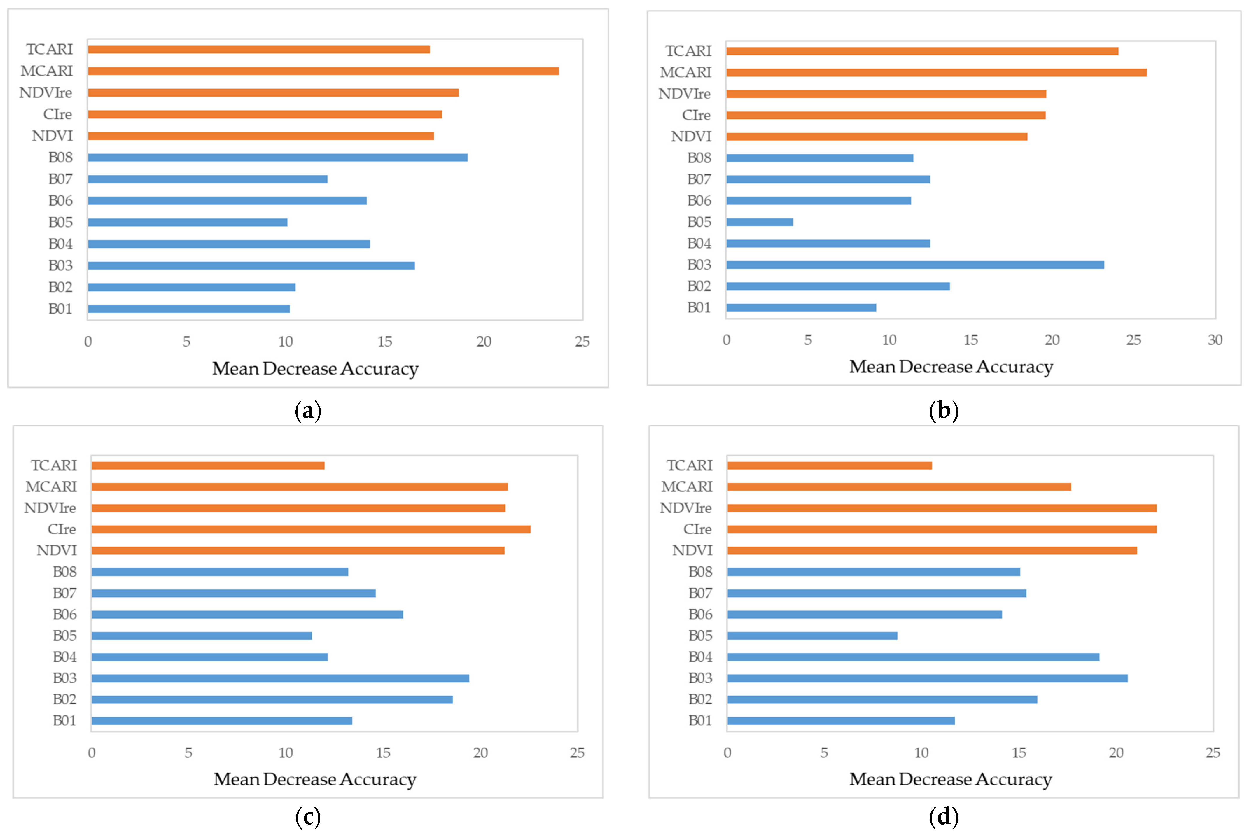
The importance of eight spectral bands and five VIs in four phases was measured by the mean decrease accuracy method, and the importance scores of thirteen features were obtained, respectively (Figure 4).
  • Importance analysis of spectral features in each phase
The most important spectral bands of the images on 2 January and 19 August are located in the near-infrared and red-light regions, while the most important regions on 30 March and 24 July are the red and green bands. The importance of the red-edge band is ranked fifth on 2 January and in fourth place for other phases.
2.
Importance analysis of VIs in each phase
VIs are the most important features of each phase. Taking the image on March 30 as an example, except for the red band, the top six features are all VIs. Compared with NDVI, the red-edge VIs are at the forefront. In January, March, July, and August images, NDVI ranks fourth, fifth, fourth, and third, respectively, among the five VIs. The top two VIs of January, March, July, and August are MCARI and NDVIre, MCARI and TCARI, CIre and MCARI, and CIre and NDVIre, respectively.

3.2. Vegetation Classification Results

3.2.1. Multiscale Segmentation Results

As the first step of OBIA, multiscale segmentation was carried out. The segmentation scale is the most important parameter, which seriously affects the results of vegetation classification. The “trial and error” method was used to segment the image [49,50]. Based on the ZY1-02D VNIR image synchronized with the field survey time on 30 March, the near-infrared, red, green, and blue bands were used as inputs, and the weight of each band was set to 1. Through the “trial and error” method and previous research experience [51,52], the scales were set to 25, 50, and 100, respectively, and the appropriate segmentation scale was determined by the classification accuracy under the conditions of spectral parameter of 0.9, shape parameter of 0.1, compactness of 0.5 and smoothness of 0.5 (Table 5).
The segmentation scale of 50 is suitable with the highest classification accuracy. According to the segmentation results in Figure 5, it can be seen that when the scale parameter is too small, which is 25, the object is too fragmented. Once it is too big, such as a scale of 100, for vegetation types with similar spatial and spectral features, it will increase the probability that the object contains different vegetation types.

3.2.2. Classification Results of Single-Temporal Red-Edge VIs

According to the single-temporal classification schemes in Section 2.2.4, a total of 24 schemes of A, AB, AC, AD, AE, and AF for four phases were carried out based on the RF algorithm. The OA and Kappa coefficient of different schemes are shown in Figure 6, and the classification accuracies of different vegetation types in each phase are shown in Table 6, Table 7, Table 8 and Table 9. McNemar’s test χ2 values for pair comparisons of the classification schemes of each image are shown in Table 10.
Through McNemar’s test, all the single-temporal classification schemes listed in Table 10 have significant differences apart from the test between scheme AB and AF in March, based on which, we can analyze the accuracy differences between different classification schemes.
In January, the OA of the 4-band was 72.03%, and the OA of the 5-band ranged from 72.71% to 76.43%, all of which improved the classification accuracy to a certain extent, among which the accuracy of the MCARI-assisted scheme was the highest, with an increase of more than 4%, followed by CIre. In March, the OA of the 4-band was 81.76%, and the OA of the 5-band ranged from 80.92% to 86.29%. The Cire-, NDVIre-, and MCARI-assisted schemes improved the accuracy, among which NDVIre improved the accuracy by more than 4%, followed by CIre. In July, the OA of the 4-band was 77.84%, and the OA of the 5-band ranged from 76.39% to 79.29%. The three schemes of CIre, NDVIre, and MCARI improved the accuracies, among which CIre improved the accuracy the most, with the accuracy increased by 1.45%, followed by NDVIre. In August, the OA of the 4-band was 77.62%, the OA of the 5-band ranged from 76.05% to 81.55%, and the accuracies of the Cire-, NDVIre-, and NDVI-assisted schemes were improved, among which NDVIre had the highest accuracy, with an improvement of nearly 4%, followed by CIre. Generally speaking, the classification results are consistent with the feature importance evaluations, and the red-edge VIs have a stronger ability to improve vegetation classification than NDVI. Among the four red-edge VIs, CIre and NDVIre acquire better vegetation classification results.
Compared with the vegetation classification results of January, July, and August, the image classification accuracy of 30 March is the highest, and the OA of different classification schemes reaches 80.92% to 86.29%, which is related to the fact that the image time is consistent with the field survey time and the difference among vegetation types in March is greater than that in January, July, and August. The seasons of 24 July and 19 August are similar, and just have a little difference in classification accuracy. The image of 2 January has the lowest accuracy.
In terms of the vegetation types, the accuracies of dry land and garden are poor in January, July, and August, and better in March, reaching 79.87% and 89.28%, respectively, in the classification of the NDVIre-assisted scheme. The woodland and paddy field have achieved good results in all four phases. The highest accuracies are 90.60% for woodland in August and 84.31% for paddy fields in January, respectively.

3.2.3. Classification Results of Multi-Temporal Red-Edge VIs

According to the multi-temporal classification schemes in Section 2.2.4, a total of five schemes of A2B, A2C, A2D, A2E, and A2F were carried out based on the RF algorithm. The vegetation classification accuracies of different multi-temporal VIs are shown in Table 11. McNemar’s test χ2 values for pair comparisons of the classification schemes of multi-temporal red-edge Vis-assisted classifications are shown in Table 12.
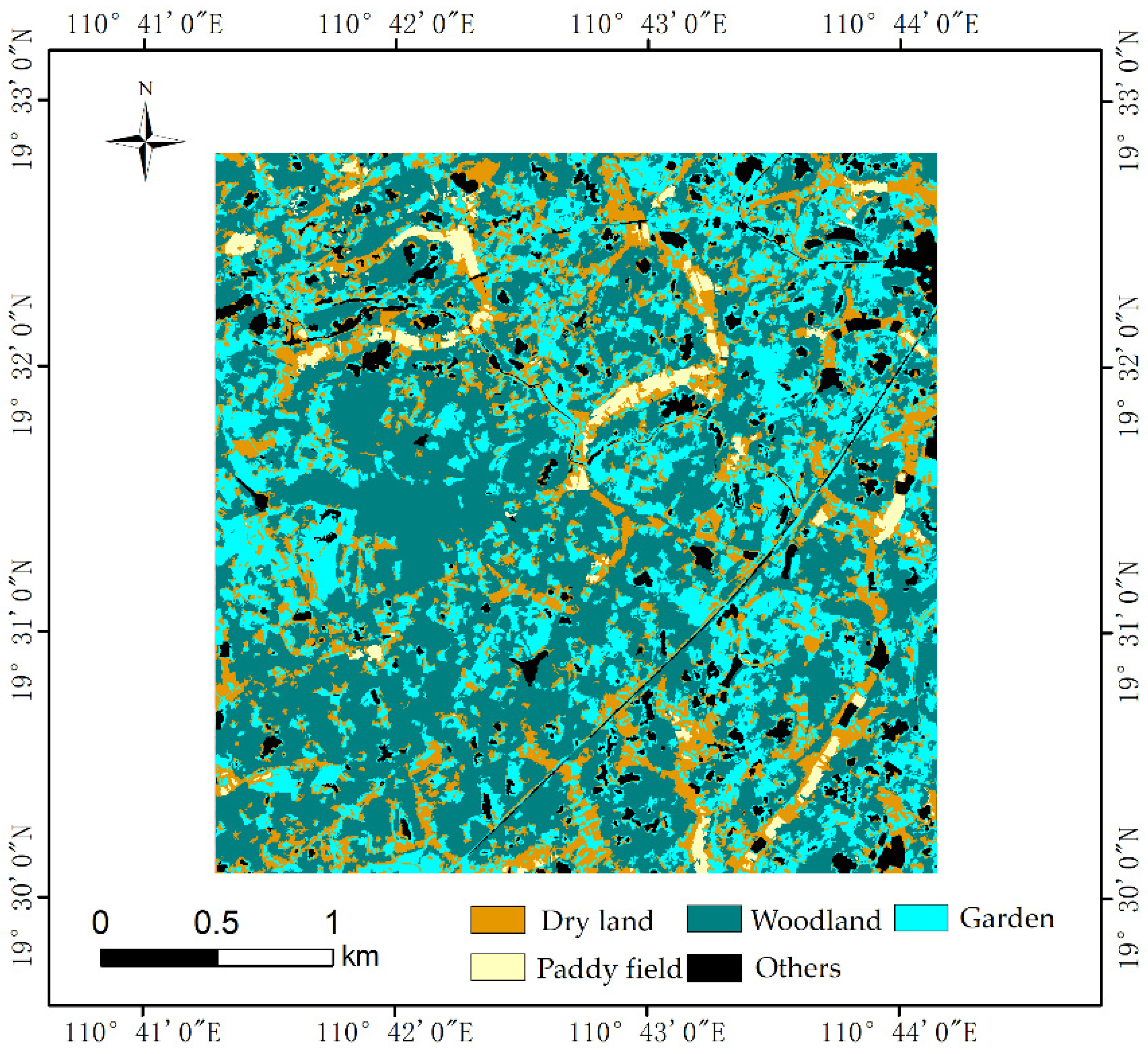
Through McNemar’s test, all the different classification schemes listed in Table 12 have significant differences apart from the test between schemes A2B and A2E. The classification accuracy of the multi-temporal schemes is improved from 86.29% of the highest single-temporal accuracy to 92.36%, an increase of 6%. Among them, multi-temporal Cire- and NDVIre-assisted schemes achieve the highest accuracies, followed by TCARI, MCARI, and NDVI, and the difference in accuracy between MCARI- and NDVI-assisted schemes is not statistically significant. The vegetation classification result of the multi-temporal Cire-assisted scheme is shown in Figure 7, which shows the specific categories of each pixel.

4. Discussion

Vegetation leaf surface has strong absorption characteristics in the red band of visible light and strong reflection characteristics in the near-infrared band, which is the physical basis of vegetation remote sensing monitoring. Based on the above characteristics of vegetation in the visible near-infrared band, five VIs, including four red-edge VIs were calculated from different combinations of spectral bands to analyze their performance in vegetation classification.
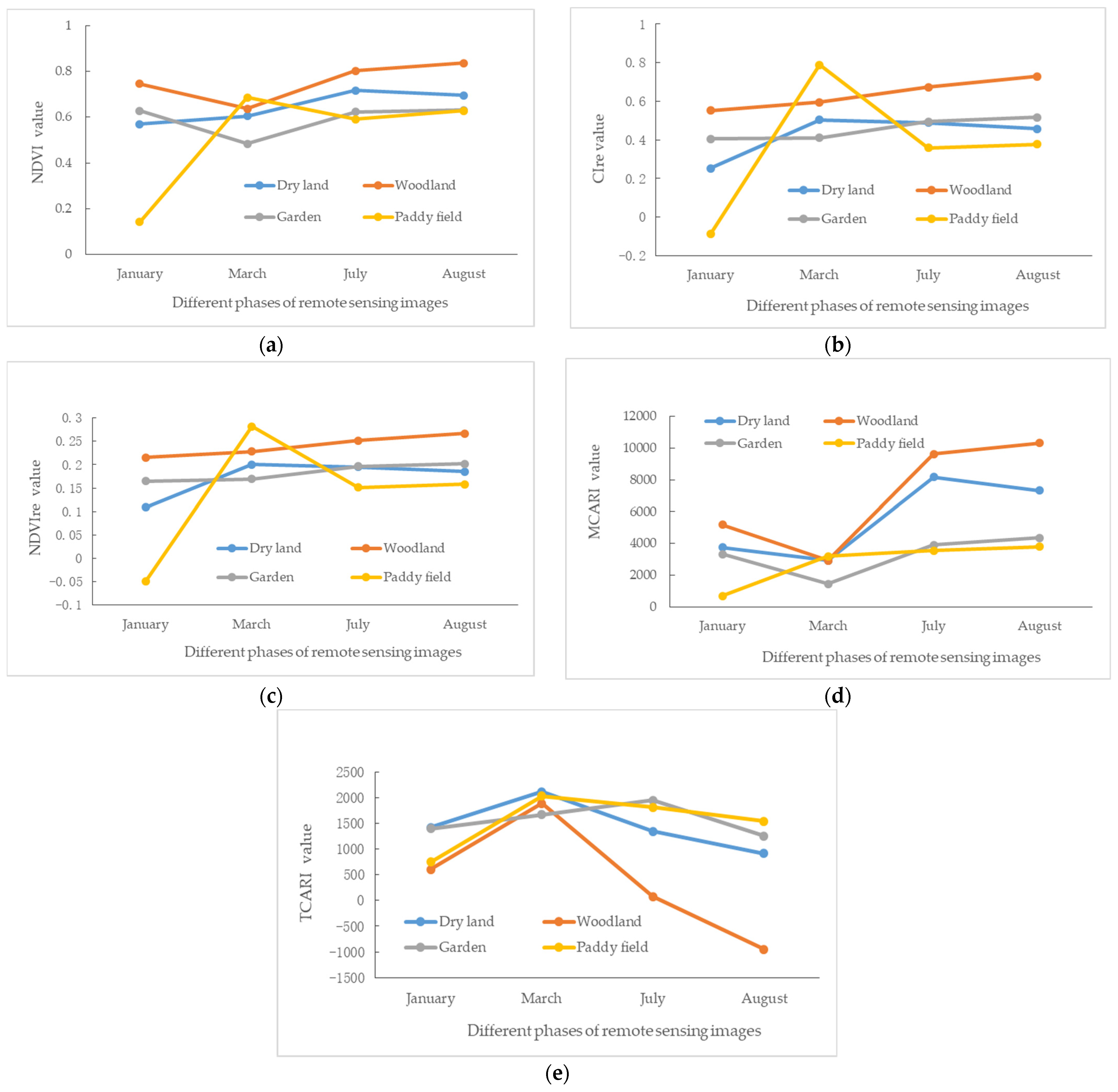
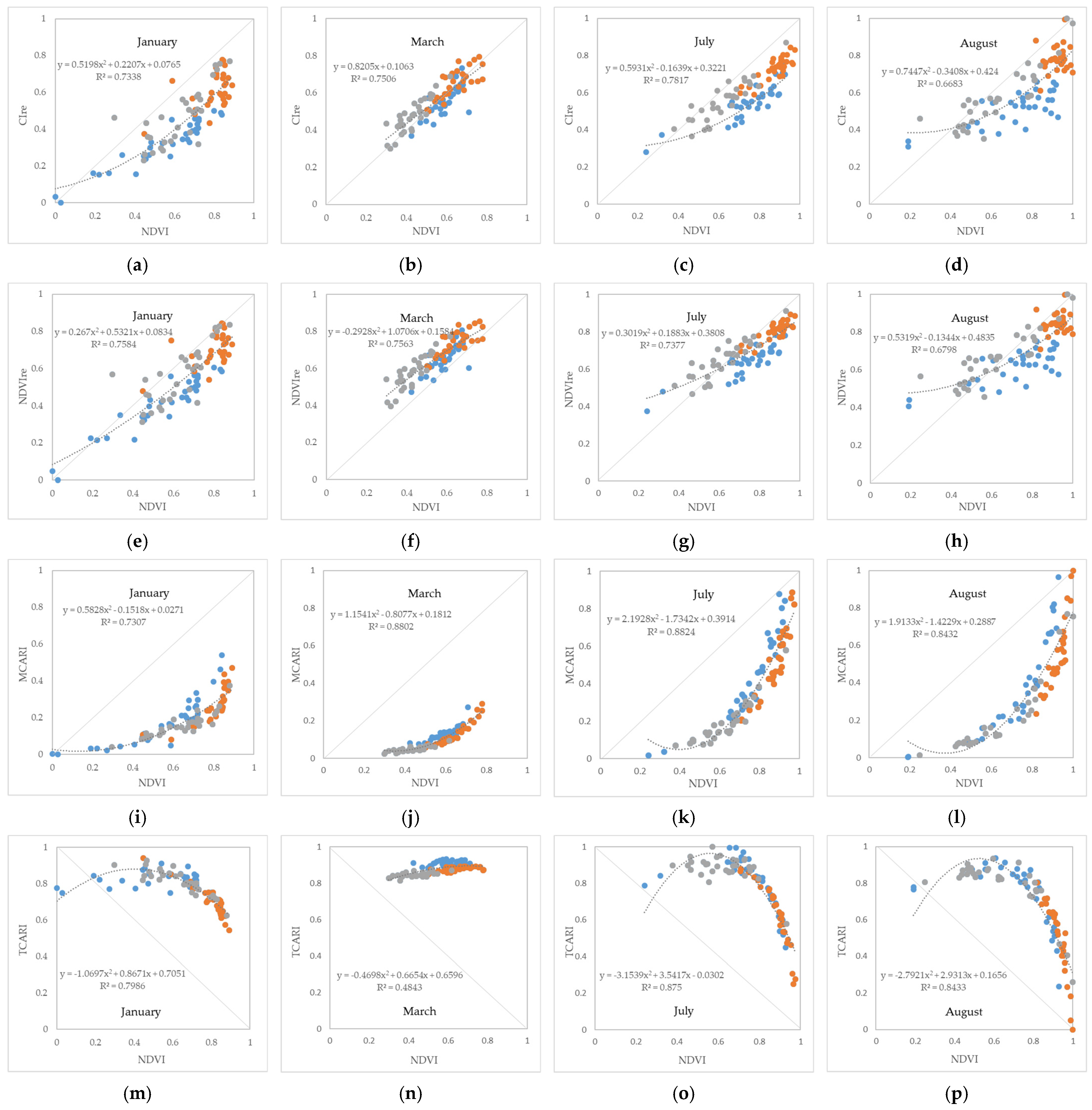
The variation and saturation of VIs for various vegetation types with different seasons were analyzed. On the one hand, based on the training samples of various vegetation types (dry land, woodland, garden, and paddy field) shown in Table 2, with a total of 123 polygons, the mean values of VIs for various vegetation types were calculated and the changes in the five VIs on four phases were plotted (Figure 8). On the other hand, in order to facilitate the comparison between red-edge VIs and NDVI, the VIs of January, March, July, and August were normalized for each vegetation type. It is worth noting that because some rice was harvested in July and August, only three types of dry land, woodland, and garden, a total of 93 polygon samples are contained. With normalized NDVI as the abscissa and normalized CIre, NDVIre, MCARI, and TCARI as the ordinates, respectively, the scatter plots of the relationship between each red-edge vegetation index and NDVI with different seasons were drawn (Figure 9).
As shown in Figure 8, in the rapid growth stage of various vegetation types from March to July, the VIs of NDVI, MCARI, and TCARI increased more than those of CIre and NDVIre. At the same time, from July to August, the VIs of NDVI and MCARI changed slightly, that is, they reached saturation more quickly. According to the scatter plot of Figure 9, CIre, NDVIre, and MCARI are positively correlated with NDVI, among which MCARI in March, July, and August shows a strong correlation with NDVI. TCARI in January, July, and August is negatively correlated with NDVI. In July and August, when the vegetation growth almost reached the peak, the normalized numerical scatters of each red-edge VI deviated from the 1: 1 standard line, showing a state of better anti-saturation performance than NDVI. This is consistent with the research results of Sun [53], who established the hyperspectral image-based vegetation index (HSVI), which obtained a high correlation with NDVI and could effectively alleviate the saturation problem caused by high vegetation coverage.
Through Figure 9, we can also analyze the separability of various vegetation types. It can be seen from the scatter plots that the vegetation in January, July, and August are more dispersed and the intersection situation is more serious than that in March, which also explains why the classification accuracy in March is higher. In early January, crops such as peanuts are in planting season, and winter melons and vegetables are in the harvesting stage, which increases the confusion between the types of dry land and others. In gardens such as lychee, those before controlling shoot branching would increase the confusion with woodland and those after the controlling would increase the confusion with dry land. At the end of March, the garden is still in the spring controlling shoot branching stage, the forest leaves have begun to grow, and the differences among vegetation types increase, which promotes classification accuracy. With the growth of vegetation, in July and August, when the growth of vegetation tends to peak, the VIs of vegetation are concentrated in the high-value range, which reduces the separability between different vegetation types and lowers the classification accuracy. At this time, the red-edge VIs with better anti-saturation performance than NDVI tend to obtain higher accuracy in vegetation classification, such as CIre and NDVIre, which has been verified in previous study [54]. However, we should also see that in this study area, although the anti-saturation performance of MCARI and TCARI is also better than NDVI, the confusion between garden and dry land, and woodland and dry land has also increased significantly.
Therefore, according to the classification accuracy of each vegetation index and the analysis of its saturation state, Cire- or NDVIre-assisted models can be used to classify vegetation in tropical monsoon regions to ensure the accuracies, especially in the rapid growth stage of vegetation where VIs are easily saturated. In this study, the classification accuracy has a certain correlation with the anti-saturation performance. It seems that the stronger the ability of VIs to improve classification accuracy, the better its anti-saturation performance. But the reverse is not necessarily true, that is, the stronger the anti-saturation performance of VIs, the classification accuracy does not necessarily tend to be better. This requires a comprehensive analysis with other factors such as the inter-class separability of VIs.

5. Conclusions

In this study, we try to evaluate the accuracy changes in several red-edge VIs on vegetation classification in tropical monsoon regions and analyze their anti-saturation performance. Taking the Wenchang study area in Hainan, China as an example, we have extracted NDVI and four red-edge VIs of CIre, NDVIre, MCARI and TCARI by using the 2.5 m fused images of ZY-102D in January, March, July and August. The significant differences between various classification schemes were carried out by McNemar’s test. The results show that the classification accuracy of NDVI-assisted schemes has little change, with only a slight improvement in two phases. Consistent with the previous research results, the red-edge information can improve the accuracy of vegetation classification. For the four phases in the study area, the vegetation classification accuracy achieves the highest with the participation of the red-edge VIs, which proves the effectiveness of the red-edge VIs in the vegetation classification in tropical monsoon regions. Among them, CIre and NDVIre are robust and improve the classification accuracy in all single-temporal and multi-temporal classifications. In the analysis of the saturation state of red-edge VIs, we find that the increase in VIs gradually slows down with the growth of vegetation, and by August, NDVI, MCARI, etc., tend to be saturated. According to the scatter plots between the normalized red-edge VIs and NDVI, we find that the anti-saturation performance of each red-edge vegetation index is better than NDVI. After further analyzing the seasonal changes in red-edge VIs, it can be found that the robust red-edge VIs, such as CIre and NDVIre, which can effectively improve the classification accuracy in each phase, are not only difficult to saturate in the month when vegetation growth is near the peak, but also can ensure the separability of different vegetation types.
Several directions for future research are clear. First of all, in this study, only images of 2 January, 30 March, 24 July, and 19 August 2021 were collected in the study area, without images of rapid vegetation growth in May, peak vegetation growth in September, and vegetation decline in October. Therefore, it is particularly necessary to add more phases to analyze the seasonal change in vegetation growth and the saturation of red-edge VIs. It is a challenge to fuse the temporal and spatial features of the red-edge band, construct the time series spectrum of red-edge VIs with high resolution, and make up for the phase deficiency of high-resolution images. In addition, this study only discussed the validity and anti-saturation performance of four kinds of red-edge VIs, namely CIre, NDVIre, MCARI, and TCARI. According to the changes in the reflective spectra of various vegetation types with the seasons, the new red-edge vegetation index with strong anti-saturation performance for tropical vegetation is worth looking forward to, so as to deepen the understanding and cognitive improvement of the mechanism to promote classification, and strengthen the effective application of red-edge VIs in tropical vegetation classification.
Author Contributions

Conceptualization, J.Y., Y.Z. and X.G.; methodology, M.L. and J.Y.; investigation and data acquisition, M.L. and Y.K.; data analysis and original draft preparation, M.L., Y.Z., J.L. and X.S.; validation, writing, review and editing, X.W., C.W., L.L. and H.G.; All authors contributed to the discussion, provided suggestions to improve the manuscript and checked the writing. All authors have read and agreed to the published version of the manuscript.

Funding

This study was funded by the Hainan Provincial Natural Science Foundation of China (322QN347), the Major Project of High-Resolution Earth Observation System (30-Y60B01-9003-22/23) and the Common Application Support Platform for National Civil Space Infrastructure Land Observation Satellites (2017-000052-73-01-001735).

Data Availability Statement

Data are contained within the article.

Conflicts of Interest

The authors declare no conflicts of interest.

References

  1. Wang, J.; Huang, J.; Zhang, K.; Li, X.; She, B.; Wei, C.; Gao, J.; Song, X. Rice fields mapping in fragmented area using multi-temporal HJ-1A/B CCD images. Remote Sens. 2015, 7, 3467–3488. [Google Scholar] [CrossRef]
  2. Domaç, A.; Süzen, M. Integration of environmental variables with satellite images in regional scale vegetation classification. Int. J. Remote Sens. 2006, 27, 1329–1350. [Google Scholar] [CrossRef]
  3. Tucker, C.J. Red and photographic infrared linear combinations for monitoring vegetation. Remote Sens. Environ. 1979, 8, 127–150. [Google Scholar] [CrossRef]
  4. Tucker, C.J.; Elgin, J.H.; Iii, M.M.; Fan, C.J. Monitoring corn and soybean crop development with hand-held radiometer spectral data. Remote Sens. Environ. 1979, 8, 237–248. [Google Scholar] [CrossRef]
  5. Camps-Valls, G.; Campos-Taberner, M.; Moreno-Martínez, Á.; Walther, S.; Duveiller, G.; Cescatti, A.; Mahecha, M.D.; Muñoz-Marí, J.; García-Haro, F.J.; Guanter, L.; et al. A unified vegetation index for quantifying the terrestrial biosphere. Sci. Adv. 2021, 7, eabc7447. [Google Scholar] [CrossRef] [PubMed]
  6. Jiang, Z.; Huete, A.R.; Didan, K.; Miura, T. Development of a 2-band enhanced vegetation index without a blue band. Remote Sens. Environ. 2008, 112, 3833–3845. [Google Scholar] [CrossRef]
  7. Lin, S.; Liu, R. A simple method to extract tropical monsoon forests using NDVI based on MODIS data: A case study in South Asia and Peninsula Southeast Asia. Chin. Geogr. Sci. 2016, 26, 22–34. [Google Scholar] [CrossRef]
  8. Zhu, Q.; Guo, H.; Zhang, L.; Liang, D.; Liu, X.; Wan, X.; Liu, J. Tropical Forests Classification Based on Weighted Separation Index from Multi-Temporal Sentinel-2 Images in Hainan Island. Sustainability 2021, 13, 13348. [Google Scholar] [CrossRef]
  9. Qin, Y.; Xiao, X.; Dong, J.; Zhang, G.; Roy, P.S.; Joshi, P.K.; Gilani, H.; Murthy, M.S.R.; Jin, C.; Wang, J. Mapping forests in monsoon Asia with ALOS PALSAR 50-m mosaic images and MODIS imagery in 2010. Sci. Rep. 2016, 6, 20880. [Google Scholar] [CrossRef]
  10. Stibig, H.; Beuchle, R.; Achard, F. Mapping of the tropical forest cover of insular Southeast Asia from SPOT4-Vegetation images. Int. J. Remote Sens. 2003, 24, 3651–3662. [Google Scholar] [CrossRef]
  11. Dong, J.; Xiao, X.; Sheldon, S.; Biradar, C.; Xie, G. Mapping tropical forests and rubber plantations in complex landscapes by integrating PALSAR and MODIS imagery. ISPRS J. Photogramm. Remote Sens. 2012, 74, 20–33. [Google Scholar] [CrossRef]
  12. Nguyen Trong, H.; Nguyen, T.D.; Kappas, M. Land cover and forest type classification by values of vegetation indices and forest structure of tropical lowland forests in central Vietnam. Int. J. For. Res. 2020, 2020, 8896310. [Google Scholar] [CrossRef]
  13. Zhang, L.; Wan, X.; Sun, B. Tropical natural forest classification using time-series Sentinel-1 and Landsat-8 images in Hainan Island. In Proceedings of the IGARSS 2019—2019 IEEE International Geoscience and Remote Sensing Symposium, Yokohama, Japan, 28 July–2 August 2019. [Google Scholar]
  14. De Alban, J.D.T.; Connette, G.M.; Oswald, P.; Webb, E.L. Combined Landsat and L-band SAR data improves land cover classification and change detection in dynamic tropical landscapes. Remote Sens. 2018, 10, 306. [Google Scholar] [CrossRef]
  15. Qin, Z.; Chang, Q.; Shen, J.; Yu, Y.; Liu, J. Red Edge Characteristics and SPAD Estimation Model Using Hyperspectral Data for Rice in Ningxia Irrigation Zone. Geomat. Inf. Sci. Wuhan Univ. 2016, 41, 1168–1175. [Google Scholar]
  16. Cho, M.A.; Skidmore, A.K.; Atzberger, C. Towards red-edge positions less sensitive to canopy biophysical parameters for leaf chlorophyll estimation using properties optique spectrales des feuilles (PROSPECT) and scattering by arbitrarily inclined leaves (SAILH) simulated data. Int. J. Remote Sens. 2008, 29, 2241–2255. [Google Scholar] [CrossRef]
  17. Kanke, Y.; Tubaña, B.; Dalen, M.; Harrell, D. Evaluation of red and red-edge reflectance-based vegetation indices for rice biomass and grain yield prediction models in paddy fields. Precis. Agric. 2016, 17, 507–530. [Google Scholar] [CrossRef]
  18. Delegido, J.; Verrelst, J.; Meza, C.M.; Rivera, J.P.; Alonso, L.; Moreno, J. A red-edge spectral index for remote sensing estimation of green LAI over agroecosystems. Eur. J. Agron. 2013, 46, 42–52. [Google Scholar] [CrossRef]
  19. Üstüner, M.; Sanli, F.B.; Abdikan, S.; Esetlili, M.T.; Kurucu, Y. Crop Type Classification Using Vegetation Indices of RapidEye Imagery. ISPRS Int. Arch. Photogramm. Remote Sens. Spat. Inf. Sci. 2014, 40, 195–198. [Google Scholar] [CrossRef]
  20. Jing, W.U.; Yuna, L.; Chunbin, L.I.; Quanhong, L.I. Fine Classification of County Crops Based on Multi-temporal Images of Sentinel-2A. Trans. Chin. Soc. Agric. Mach. 2019, 50, 194–200. [Google Scholar]
  21. Jianwen, H.; Zengyuan, L.; Erxue, C.; Lei, Z.; Bingping, M. Classification of plantation types based on WFV multispectral imagery of the GF-6 satellite. Natl. Remote Sens. Bull. 2021, 25, 539–548. [Google Scholar]
  22. Yan, E.; Wang, G.; Lin, H.; Xia, C.; Sun, H. Phenology-based classification of vegetation cover types in Northeast China using MODIS NDVI and EVI time series. Int. J. Remote Sens. 2015, 36, 489–512. [Google Scholar] [CrossRef]
  23. Zheng, H.; Cheng, T.; Yao, X.; Deng, X.; Tian, Y.; Cao, W.; Zhu, Y. Detection of rice phenology through time series analysis of ground-based spectral index data. Field Crops Res. 2016, 198, 131–139. [Google Scholar] [CrossRef]
  24. Cooley, T.; Anderson, G.P.; Felde, G.W.; Hoke, M.L.; Ratkowski, A.J.; Chetwynd, J.H.; Gardner, J.A.; Adler-Golden, S.M.; Matthew, M.W.; Berk, A. FLAASH, a MODTRAN4-based atmospheric correction algorithm, its application and validation. In Proceedings of the IEEE International Geoscience and Remote Sensing Symposium, Toronto, ON, Canada, 24–28 June 2002. [Google Scholar]
  25. Ke, Y.; Im, J.; Lee, J.; Gong, H.; Ryu, Y. Characteristics of Landsat 8 OLI-derived NDVI by comparison with multiple satellite sensors and in-situ observations. Remote Sens. Environ. 2015, 164, 298–313. [Google Scholar] [CrossRef]
  26. Laben, C.A.; Brower, B.V. Process for Enhancing the Spatial Resolution of Multispectral Imagery Using Pan-Sharpening. U.S. Patent 6011875, 4 January 2000. [Google Scholar]
  27. Rouse, J.W., Jr.; Haas, R.H.; Schell, J.A.; Deering, D.W. Monitoring the Vernal Advancement and Retrogradation (Green Wave Effect) of Natural Vegetation; Remote Sensing Center, Texas A&M University: College Station, TX, USA, 1973. [Google Scholar]
  28. Gitelson, A.A.; Gritz, Y.; Merzlyak, M.N. Relationships between leaf chlorophyll content and spectral reflectance and algorithms for non-destructive chlorophyll assessment in higher plant leaves. J. Plant Physiol. 2003, 160, 271–282. [Google Scholar] [CrossRef] [PubMed]
  29. Gitelson, A.A.; Keydan, G.P.; Merzlyak, M.N. Three-band model for noninvasive estimation of chlorophyll, carotenoids, and anthocyanin contents in higher plant leaves. Geophys. Res. Lett. 2006, 33. [Google Scholar] [CrossRef]
  30. Barnes, E.M.; Clarke, T.R.; Richards, S.E.; Colaizzi, P.D.; Thompson, T. Coincident detection of crop water stress, nitrogen status, and canopy density using ground based multispectral data. In Proceedings of the 5th International Conference on Precision Agriculture and Other Resource Management, Bloomington, MN, USA, 16–19 July 2000. [Google Scholar]
  31. Daughtry, C.S.T.; Walthall, C.L.; Kim, M.S.; Colstoun, E.B.D.; Iii, M.M. Estimating corn leaf chlorophyll concentration from leaf and canopy reflectance. Remote Sens. Environ. 2000, 74, 229–239. [Google Scholar] [CrossRef]
  32. Haboudane, D.; Miller, J.R.; Tremblay, N.; Zarco-Tejada, P.J.; Dextraze, L. Integrated narrow-band vegetation indices for prediction of crop chlorophyll content for application to precision agriculture. Remote Sens. Environ. 2002, 81, 416–426. [Google Scholar] [CrossRef]
  33. Bruzzone, L.; Roli, F. An extension of the Jeffreys-Matusita distance to multiclass cases for feature selection. IEEE Trans. Geosci. Remote Sens. 1995, 33, 1318–1321. [Google Scholar] [CrossRef]
  34. Hao, P.; Wu, M.; Niu, Z.; Wang, L.; Zhan, Y. Estimation of different data compositions for early-season crop type classification. PeerJ 2018, 6, e4834. [Google Scholar] [CrossRef]
  35. Breiman, L. Random Forests. Mach. Learn. 2001, 45, 5–32. [Google Scholar] [CrossRef]
  36. Strobl, C.; Boulesteix, A.L.; Kneib, T.; Augustin, T.; Zeileis, A. Conditional variable importance for random forests. BMC Bioinform. 2008, 9, 307. [Google Scholar] [CrossRef] [PubMed]
  37. Gislason, P.O.; Benediktsson, J.A.; Sveinsson, J.R. Random Forests for land cover classification. Pattern Recognit. Lett. 2006, 27, 294–300. [Google Scholar] [CrossRef]
  38. Piazza, G.A.; Vibrans, A.C.; Liesenberg, V.; Refosco, J.C. Object-oriented and pixel-based classification approaches to classify tropical successional stages using airborne high–spatial resolution images. GIScience Remote Sens. 2016, 53, 206–226. [Google Scholar] [CrossRef]
  39. De Giglio, M.; Greggio, N.; Goffo, F.; Merloni, N.; Dubbini, M.; Barbarella, M. Comparison of Pixel- and Object-Based Classification Methods of Unmanned Aerial Vehicle Data Applied to Coastal Dune Vegetation Communities: Casal Borsetti Case Study. Remote Sens. 2019, 11, 1416. [Google Scholar] [CrossRef]
  40. Han, N.; Wang, K.; Yu, L.; Zhang, X. Integration of texture and landscape features into object-based classification for delineating Torreya using IKONOS imagery. Int. J. Remote Sens. 2012, 33, 2003–2033. [Google Scholar] [CrossRef]
  41. Haralock, R.M.; Shapiro, L.G. Computer and Robot Vision; Addison-Wesley Longman Publishing Co., Inc.: Boston, MA, USA, 1991. [Google Scholar]
  42. Cheng, J.; Bo, Y.; Zhu, Y.; Ji, X. A novel method for assessing the segmentation quality of high-spatial resolution remote-sensing images. Int. J. Remote Sens. 2014, 35, 3816–3839. [Google Scholar] [CrossRef]
  43. Benz, U.C.; Hofmann, P.; Willhauck, G.; Lingenfelder, I.; Heynen, M. Multi-resolution, object-oriented fuzzy analysis of remote sensing data for GIS-ready information. ISPRS J. Photogramm. Remote Sens. 2011, 58, 239–258. [Google Scholar] [CrossRef]
  44. Htitiou, A.; Boudhar, A.; Lebrini, Y.; Hadria, R.; Benabdelouahab, T. The Performance of Random Forest Classification Based on Phenological Metrics Derived from Sentinel-2 and Landsat 8 to Map Crop Cover in an Irrigated Semi-arid Region. Remote Sens. Earth Syst. Sci. 2019, 2, 208–224. [Google Scholar] [CrossRef]
  45. Kvalseth, T.O. A coefficient of agreement for nominal scales: An asymmetric version of Kappa. Educ. Psychol. Meas. 1991, 51, 95–101. [Google Scholar] [CrossRef]
  46. Congalton, R.G. A review of assessing the accuracy of classifications of remotely sensed data. Remote Sens. Environ. 1991, 37, 35–46. [Google Scholar] [CrossRef]
  47. Edwards, A.L. Note on the “correction for continuity” in testing the significance of the difference between correlated proportions. Psychometrika 1948, 13, 185–187. [Google Scholar] [CrossRef] [PubMed]
  48. Foody, G.M. Thematic map comparison: Evaluating the Statistical Significance of Differences in Classification Accuracy. Photogramm. Eng. Remote Sens. 2004, 70, 627–633. [Google Scholar] [CrossRef]
  49. Qian, Y.; Zhou, W.; Yan, J.; Li, W.; Han, L. Comparing machine learning classifiers for object-based land cover classification using very high resolution imagery. Remote Sens. 2015, 7, 153–168. [Google Scholar] [CrossRef]
  50. Zhou, W.; Troy, A. An object-oriented approach for analysing and characterizing urban landscape at the parcel level. Int. J. Remote Sens. 2008, 29, 3119–3135. [Google Scholar] [CrossRef]
  51. Pu, R.; Landry, S.; Yu, Q. Object-based urban detailed land cover classification with high spatial resolution IKONOS imagery. Int. J. Remote Sens. 2011, 32, 3285–3308. [Google Scholar] [CrossRef]
  52. Laliberte, A.S.; Rango, A.; Havstad, K.M.; Paris, J.F.; Beck, R.F.; McNeely, R.; Gonzalez, A.L. Object-oriented image analysis for mapping shrub encroachment from 1937 to 2003 in southern New Mexico. Remote Sens. Environ. 2004, 93, 198–210. [Google Scholar] [CrossRef]
  53. Sun, G.; Jiao, Z.; Zhang, A.; Li, F.; Fu, H.; Li, Z. Hyperspectral image-based vegetation index (HSVI): A new vegetation index for urban ecological research. Int. J. Appl. Earth Obs. Geoinf. 2021, 103, 102529. [Google Scholar] [CrossRef]
  54. Kang, Y.; Meng, Q.; Liu, M.; Zou, Y.; Wang, X. Crop classification based on red edge features analysis of GF-6 WFV data. Sensors 2021, 21, 4328. [Google Scholar] [CrossRef]
Figure 1. Geographic location and sample distribution of the study area.
Remotesensing 16 01865 g001
Figure 2. Technical route of the study.
Remotesensing 16 01865 g002
Figure 3. JBh distance for two spectral analysis schemes at 4-band and 5-band in different phases of remote sensing images. The Y-axis is the Jbh distance value, indicating the separability of vegetation types. A total of 43,104 samples in 5 categories are used to calculate the Jbh distance.
Remotesensing 16 01865 g003
Figure 4. Importance evaluation results of the spectra and VIs for each phase. The results of VIs are marked in orange and spectral results in blue. (a) January; (b) March; (c) July; (d) August.
Remotesensing 16 01865 g004
Figure 5. Local image segmentation results at different scales. The boundaries of the segmentation objects are marked with blue lines. (a) Segmentation scale: 25; (b) segmentation scale: 50; (c) segmentation scale: 100; and (d) the legend.
Remotesensing 16 01865 g005
Figure 6. Vegetation classification accuracies of different schemes in four phases. The classification schemes are shown in Table 4 with A representing 4-band, AB representing 4-band + NDVI, AC representing 4-band + CIre, AD representing 4-band + NDVIre, AE representing 4-band + MCARI, AF representing 4-band + TCARI. (a) OA; (b) Kappa.
Remotesensing 16 01865 g006
Figure 7. The vegetation classification result map of multi-temporal Cire-assisted scheme.
Remotesensing 16 01865 g007
Figure 8. Variation curves of different VIs in January, March, July, and August. The types of dry land, woodland, garden, and paddy field are marked with different colors. (a) NDVI; (b) CIre; (c) NDVIre; (d) MCARI; (e) TCARI.
Remotesensing 16 01865 g008
Figure 9. Scatter plots of the relationship between normalized red-edge VIs and NDVI for different vegetation types in January, March, July, and August. Dry land, woodland, and garden are marked with blue, orange, and grey dots, respectively. (a) CIre (January); (b) CIre (March); (c) CIre (July); (d) CIre (August); (e) NDVIre (January); (f) NDVIre (March); (g) NDVIre (July); (h) NDVIre (August); (i) MCARI (January); (j) MCARI (March); (k) MCARI (July); (l) MCARI (August); (m) TCARI (January); (n) TCARI (March); (o) TCARI (July); and (p) TCARI (August).
Remotesensing 16 01865 g009
Table 1. Main parameter information of ZY1-02D VNIR camera.
ItemsParameters
VNIR CameraSpectral RangePan0.452~0.902 υm
B010.452~0.521 υm
B020.522~0.607 υm
B030.635~0.694 υm
B040.776~0.895 υm
B050.416~0.452 υm
B060.591~0.633 υm
B070.708~0.752 υm
B080.871~1.047 υm
Spatial ResolutionPan2.5 m
B01~B0810 m
Width115 km
Table 2. Number of training and verification samples.
ClassificationNumber of Training SamplesNumber of Verification Samples
PolygonsPixelsPolygonsPixels
Dry land324049211684
Paddy field309874203554
Woodland3015,498206418
Garden314428201772
Others329255203344
Total15543,10410116,772
Table 3. VIs and calculation method.
NameCalculation Method
Normalized Difference Vegetation Index (NDVI) [27] ( ρ NIR ρ R ) / ( ρ NIR + ρ R )
Chlorophyll Index red edge (CIre) [28,29] ρ NIR / ρ RE 1 1
Normalized Difference Vegetation Index red edge (NDVIre) [30] ( ρ NIR ρ RE 1 ) / ( ρ NIR + ρ RE 1 )
Modified Chlorophyll Absorption in Reflectance Index (MCARI) [31] [ ( ρ RE 1 ρ R ) 0.2 × ( ρ RE 1 ρ G ) ] × ( ρ RE 1 / ρ R )
Transformed Chlorophyll Absorption in Reflectance Index (TCARI) [32] 3 × [ ( ρ RE 1 ρ R ) 0.2 × ( ρ RE 1 ρ G ) × ( ρ RE 1 / ρ R ) ]
Table 4. Classification schemes of different VIs.
Combined BandsJanuaryMarchJulyAugust
4-band scheme: four bands (R, G, B, NIR)Scheme A (4-band)A1A2A3A4
5-band scheme:four bands (R, G, B, NIR) + NDVIScheme AB (4-band + NDVI)AB1AB2AB3AB4
four bands (R, G, B, NIR) + red-edge indexScheme AC (4-band + CIre)AC1AC2AC3AC4
Scheme AD (4-band + NDVIre)AD1AD2AD3AD4
Scheme AE (4-band + MCARI)AE1AE2AE3AE4
Scheme AF (4-band + TCARI)AF1AF2AF3AF4
8-band scheme: four bands (R, G, B, NIR) (March) + VIs of four time seriesScheme A2B (4-band (March) + four time series NDVI)
Scheme A2C (4-band (March) + four time series CIre)
Scheme A2D (4-band (March) + four time series NDVIre)
Scheme A2E (4-band (March) + four time series MCARI)
Scheme A2F (4-band (March) + four time series MCARI)
Table 5. Appropriate scale for image segmentation. The higher OA value indicates the appropriate segmentation scale, which is highlighted in bold.
ScaleOverall Accuracy (OA)
2579.58%
5081.76%
10078.75%
Table 6. Classification accuracies of different vegetation types in January. Higher values indicate better performance, and the best result is highlighted in bold.
AccuraciesSchemes
AABACADAEAF
OA72.0373.2074.4874.2476.4372.71
Kappa0.630.640.660.660.690.64
Paddy fieldPA77.2270.9380.8680.8676.3671.66
UA91.3694.5584.7584.7594.1094.09
F183.7081.0582.7682.7684.3181.36
Dry landPA34.9144.5564.4864.7957.3343.94
UA38.5535.7042.1741.2345.3134.17
F136.6439.6450.9950.3950.6238.44
WoodlandPA83.8587.8886.4985.5686.2583.20
UA81.2287.6787.4287.9883.6386.38
F182.5187.7786.9586.7584.9284.76
GardenPA38.3746.7930.8133.6062.5947.30
UA30.9837.3254.6953.7349.1537.28
F134.2841.5239.4241.3455.0641.70
OthersPA79.8375.4472.4671.4074.3281.28
UA77.9374.9269.7970.2085.8577.90
F178.8775.1871.1070.7979.6779.55
Table 7. Classification accuracies of different vegetation types in March. Higher values indicate better performance, and the best result is highlighted in bold.
AccuraciesSchemes
AABACADAEAF
OA81.7680.9285.9586.2984.7781.21
Kappa0.760.740.810.820.790.75
Paddy fieldPA73.9371.5477.0277.0273.9371.00
UA67.0070.0678.8878.8880.4164.33
F170.2970.7977.9477.9477.0367.50
Dry landPA74.4274.4274.4874.4877.5372.21
UA82.1268.8685.6986.1172.6280.91
F178.0871.5379.6979.8774.9976.31
WoodlandPA80.8684.1588.4688.4691.4579.29
UA80.8979.8382.7383.3581.9580.61
F180.8781.9385.5085.8386.4479.94
GardenPA85.1465.3183.5886.5464.5384.86
UA91.6486.5391.9592.2090.8086.55
F188.2774.4487.5789.2875.4485.70
OthersPA93.7896.5397.8097.9298.1998.46
UA96.16100.0097.0397.0499.5499.97
F194.9698.2397.4197.4898.8699.21
Table 8. Classification accuracies of different vegetation types in July. Higher values indicate better performance, and the best result is highlighted in bold.
AccuraciesSchemes
AABACADAEAF
OA77.8477.4179.2978.7978.1676.39
Kappa0.710.700.730.720.710.69
Paddy fieldPA77.9574.7076.7576.2176.9279.91
UA83.6683.1583.9482.6081.6983.25
F180.7078.7080.1879.2879.2381.55
Dry landPA57.5360.4755.4754.6562.6555.35
UA39.3744.0144.1342.8144.3634.76
F146.7550.9449.1548.0151.9442.70
WoodlandPA80.9380.0285.3285.5181.6376.13
UA90.4691.5288.7688.2291.2090.93
F185.4385.3887.0186.8486.1582.87
GardenPA54.7363.2558.1054.6250.2555.52
UA48.6849.7451.5951.4048.0450.56
F151.5355.6954.6552.9649.1252.92
OthersPA94.8391.7294.1394.1396.0095.44
UA97.4990.5397.4797.4793.2695.33
F196.1491.1295.7795.7794.6195.38
Table 9. Classification accuracies of different vegetation types in August. Higher values indicate better performance, and the best result is highlighted in bold.
AccuraciesSchemes
AABACADAEAF
OA77.6279.1580.5881.5576.8076.05
Kappa0.700.720.740.760.690.68
Paddy fieldPA69.3976.4074.7879.2970.6869.62
UA72.9575.1483.8284.6269.6173.93
F171.1375.7679.0481.8770.1471.71
Dry landPA52.7149.7360.2060.2655.1554.73
UA37.0741.1437.1239.5139.4530.75
F143.5345.0345.9247.7346.0039.38
WoodlandPA89.7590.6185.5985.5983.6586.46
UA87.9690.5993.1493.1487.4186.89
F188.8590.6089.2189.2185.4986.67
GardenPA37.4240.4861.9761.9752.1732.68
UA59.5266.3967.5067.4186.6080.08
F145.9550.2964.6264.5865.1146.42
OthersPA97.7396.0797.7097.7094.6297.40
UA97.6788.3997.6797.6787.6797.66
F197.7092.0797.6897.6891.0197.53
Table 10. McNemar’s test χ2 values for pair comparisons of four time series images.
Time seriesSchemesAABACADAEAF
JanuaryA//////
AB40.17/////
AC143.4739.72////
AD123.4524.8610.74///
AE464.11353.45115.31143.27//
AF21.0812.1559.8946.65356.58/
MarchA//////
AB26.11/////
AC645.30837.00////
AD754.00894.0055.02///
AE202.42613.2654.4984.89//
AF20.202.96 (<3.84)707.41810.55261.74/
JulyA//////
AB10.59/////
AC131.41146.66////
AD58.1971.7862.84///
AE9.8226.4861.7819.70//
AF129.6536.62294.56199.25125.40/
AugustA//////
AB138.74/////
AC237.3557.04////
AD361.74153.99160.01///
AE22.29154.44630.00792.00//
AF197.82345.33659.21818.9723.12/
For example, “A vs. AB:40.17” means that McNemar’s test χ2 value between A and AB classification schemes is 40.17. The values greater than 3.84 indicate significant difference.
Table 11. Vegetation classification accuracies of multi-temporal VIs. Higher values indicate better performance, and the best result is highlighted in bold.
AccuraciesSchemes
A2BA2CA2DA2EA2F
OA85.9092.3692.2786.0689.13
Kappa0.810.900.900.820.85
Paddy fieldPA83.0389.8389.8356.9573.42
UA100.0097.0897.7496.2592.92
F190.7393.3193.6271.5682.03
Dry landPA81.2373.8273.8289.3690.14
UA45.2276.0075.8146.8764.86
F158.1074.8974.8061.4975.44
WoodlandPA86.76100.0099.6497.7895.88
UA93.5793.1492.5694.0690.76
F190.0496.4595.9795.8893.25
GardenPA77.8279.2779.2779.5580.00
UA80.9481.6982.0789.9088.94
F179.3580.4680.6584.4184.23
OthersPA94.0896.8697.1096.6897.46
UA100.0099.9199.91100.00100.00
F196.9598.3698.4898.3198.71
Table 12. McNemar’s test χ2 values for pair comparisons of multi-temporal red-edge VIs assisted classifications.
SchemesA2BA2CA2DA2EA2F
A2B/////
A2C874.76////
A2D860.306.32///
A2E0.33 (<3.84)698.23684.94//
A2F194.03252.19244.94346.31/
For example, “A2B vs. A2C:874.76” means that McNemar’s test χ2 value between A2B and A2C classification schemes is 874.76. The values greater than 3.84 indicate significant difference.
Disclaimer/Publisher’s Note: The statements, opinions and data contained in all publications are solely those of the individual author(s) and contributor(s) and not of MDPI and/or the editor(s). MDPI and/or the editor(s) disclaim responsibility for any injury to people or property resulting from any ideas, methods, instructions or products referred to in the content.