1. Introduction
Altimetry satellites play a crucial role in monitoring and understanding various aspects of the Earth’s oceans, including sea state. These satellites utilize advanced radar systems to measure the height of the sea surface with remarkable precision, offering valuable insights into ocean dynamics and phenomena. By emitting microwave pulses towards the Earth’s surface and recording the time taken for the signals to return, altimetry can accurately determine sea surface height variations. These data enable scientists to assess parameters such as wave height, wind speed, and ocean currents, providing vital information for weather forecasting, climate research, and maritime operations [
1]. Through continuous monitoring and analysis, altimetry satellites contribute significantly to our understanding of oceanic processes and their impact on global climate systems.
The radar altimetry measures the two-way travel time of a radar pulse between the satellite antenna and the Earth’s surface at the nadir of the spacecraft. This measurement is performed through the collection of the waveforms bounced back by the reflecting facets within the altimeter footprint. While the traditional pulse-limited radar altimeters were used to collect information on the sea level and slope [
2], the delay-Doppler concept [
3], thanks to the higher along-track resolution, has been used to obtain information of the shape, balance velocities and contribution to sea level in open waters, large ice sheets [
4,
5], marine ice thickness [
6], or lake ice [
7].
Radar echoes are intrinsically affected by speckle noise, due to coherent summation of many randomly phased scatterers from the surface [
8]. Multilooking, i.e., incoherent averaging of single look echoes, is performed in order to achieve a speckle reduction. Delay/Doppler (DD) altimetry has shown to be more effective in reducing the speckle since a higher number of looks than in the conventional radar altimeter is gained. This is due also to the high number of the individual waveforms in each Doppler bin that is, for Delay/Doppler altimeters, equal to the number of pulses in a burst [
9].
However, due to the correlation among the averaged single looks, the effective number of looks (ENL) is reduced. By definition, the ENL is the number of independent observations that are obtained by the radar from a distributed target per unit of time. The ENL can be achieved by multilooking a fixed number of echoes, thus impacting the statistical properties of the final multilooked waveform. The ENL is then a figure to quantify the speckle suppression obtained by multilooking in radar signals.
A seminal study to determine the correlation properties of consecutive pulses from nadir-looking pulse-limited radar altimeters is [
10]. The study provides a value for the maximum pulse repetition frequency for which the statistical independence of consecutive waveforms is still assured. Since the TOPEX/Poseidon Mission launched in 1992, up to the Jason altimeter series, conventional low-resolution mode (LRM) altimeters were designed to obtain uncorrelated echoes. The reason was to have efficient satellite operations in terms of power usage, at the same time maximizing the information achieved from the transmitted pulses. Following these design criteria, the pulse repetition frequency (PRF) for the Jason series was selected to be approximately 2 kHz.
Copernicus Sentinel-6 Michael Freilich is the first altimeter operating in a continuous high-rate pulse mode. This design allows the simultaneous production of low-resolution mode measurements with a pulse repetition frequency of ∼9 KHz for the Ku-band as well as the processing of high-resolution echoes on ground. S6-MF thus generates an elevated number of highly correlated single looks, with respect to the fewer number of Jason-3 uncorrelated pulses.
In the theoretical model shown in [
11], for the LRM waveforms, the average of a high number of correlated single looks (∼9KHz) provides a higher ENL with respect to the case in which fewer and almost uncorrelated single looks are averaged. From this analysis, a stronger dependence with respect to the low-PRF case of the ENL on the range gate of the multilooked waveforms emerged. This dependence was later confirmed from successive analysis performed on an extensive dataset of 5 years pseudo-LRM Cryosat-2 data taken over ocean [
12] or, more recently on high-resolution Sentinel-6 data analysis [
13]. This last work showed that, despite the fact that at higher PRFs the noise in the estimation of geophysical parameters is reduced, the significant dependence of the statistical properties on the range gate introduces significant biases in the retracked parameters using least-square estimation approach. These biases have been found to be dependent on the sea geophysical parameters and need to be properly accounted for, to ensure seamless continuity of sea level monitoring between S6-MF and Jason-3, the new and previous reference missions of the ocean surface topography satellite series.
More recently [
14], the autocorrelation properties of Sentinel-3A SAR mode waveforms over open ocean have been studied to assess the effect on the retrieval of ocean geophysical parameters at various posting rates. This study confirmed the strong dependence of the decorrelation length with the multilooked SAR mode waveforms. A similar analysis [
15], based on a theoretical model, showed the power correlation variability with respect to the waveform range gate in case of SAR mode single-look waveforms. The outcome of these studies highlights that, at high PRF, the significant variability in the statistical properties of the range gates in typical L1b 20-Hz multilooked waveforms must be properly addressed when integrating Sentinel-6/Jason-CS data in a climatological data record.
In this paper, we consolidate the correlation properties of the LR-mode waveforms as a function of the sea wave height by comparing the theoretical model in [
15] with ocean data from recent S6-MF acquisitions. The accuracy and the precision of the geophysical parameters estimated from open ocean are shown as bias of the estimation evaluated with different decimation factors with respect to the evaluation at full PRF. Finally, the behavior of the ENL in case of higher posting rate is discussed.
2. Pulse-To-Pulse Correlation Model and ENL
The evaluation of the single look correlation is described in [
15] and is here shortly summarized.
The echoes acquired by a radar altimeter are affected by speckle and the purpose of multilooking is to reduce the fluctuations due to speckle. Let denote an individual echo and the echo power obtained by multiplication of an echo signal with its complex conjugate. Since individual echoes have real and imaginary parts that are zero-mean Gaussian distributed (echoes come from backscattering of many facets, so central limit theorem applies), their power p is exponentially distributed and, consequently, its variance is equal to the square of its mean .
A multilooked echo
q is achieved by averaging
N independent echo powers:
The variance of the multilooked signal is
from which
N can be retrieved:
This result exactly holds for independent identically distributed (i.i.d.) power echoes. In general, due to single-look correlation and mean-power differences of the averaged waveforms, the variance of multilooked products is larger than expected.
The effective number of looks (ENL) is defined as the estimate of the effective number of statistically independent looks for the backscattered power and is upper bounded by the actual number of single look echo waveforms averaged together. The higher the ENL, the more efficient the speckle noise mitigation and, therefore, the lower the error in the final estimation of geophysical parameters.
Thus, the ENL can be computed as follows:
After some calculation, it can be shown that
where
denotes the correlation coefficients (also called coherence) of the power echoes
and
. In case of low-resolution mode, the pulse-limited echoes summed together in a multilook echo can be assumed drawn from the same mean, thus leading to a simplified expression for Equation (
5):
The previous assumption is reasonable if geophysical parameters are slowly variant in space and in the extent of a radar cycle.
The power echoes coherence as a function of the delay
can be computed by evaluating the correlation between two identical echoes, observed with a small along-track displacement
x:
At the denominator of Equation (
7), we have the mean echo power obtained by the triple convolution of the point-target impulse response
, the sea-surface height probability density function
, which accounts for the dependence on the significant wave height (SWH), and the surface impulse response
, defined in [
16]. At the numerator of the equation, we have the covariance
, which is given again by a triple convolution but instead of the surface impulse response there is the covariance impulse response
given by [
4]:
where
is the carrier wavelength,
the antenna gain,
c the light speed,
the ocean backscattering coefficient,
h is the satellite altitude, and
with
R being the Earth radius is a geometric correction factor for the spherical surface.
H is the Heaviside step function and the last term is a circular integration along an isorange line, with
being the carrier wavenumber and
and
the antenna illumination width in the along- and across-track directions.
As can be seen from Equation (
7), the power correlation is a function of both the delay time
and the along track distance
x at which the echoes are placed, and depends on the SWH as a consequence of the convolution with the sea-surface height probability density function
. Starting from Equation (
7), the power correlation can be computed using numerical integration for different delay times
and different along track displacements
x, accounting for that the actual satellite displacement in along track direction between each pair of pulses depends on PRF and satellite velocity.
3. Power Correlation Analysis
In the following, the pulse-to-pulse autocorrelation as a function of the delay time and along-track displacement is shown for different S6-MF real datasets acquired over open ocean and in different sea conditions. In detail, different SWH are considered.
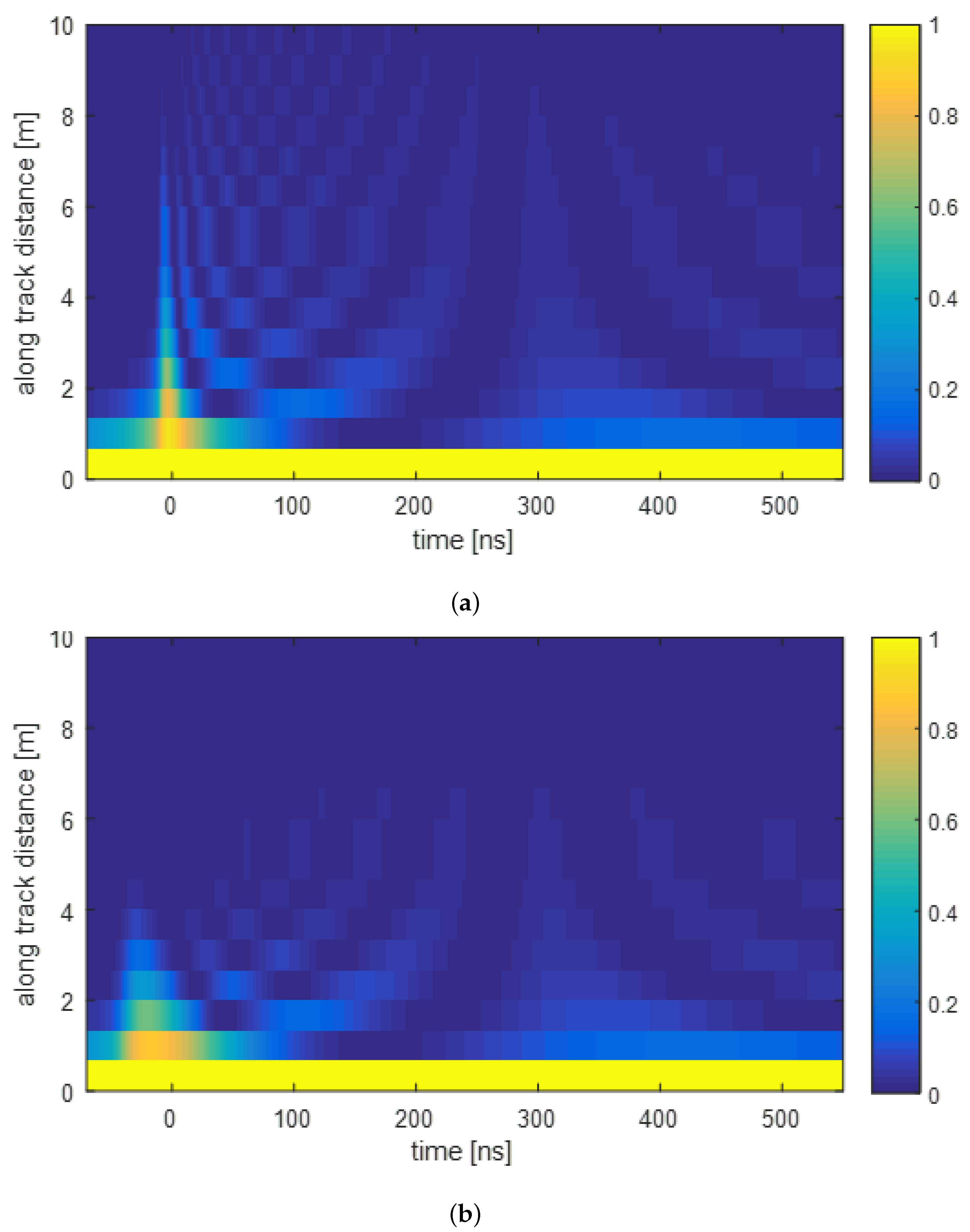
Figure 1 shows the pulse-to-pulse autocorrelation
as a function of the delay time
and the along-track displacement
x computed for S6-MF LR mode echoes for two different ocean states:
m (
Figure 1a) and
m (
Figure 1b).
It is worth remembering that the values of R are represented only for positive values of along-track displacement because the autocorrelation is symmetric with x.
As expected, the pulse-to-pulse autocorrelation is identically 1 for
(i.e., an echo is perfectly correlated with itself), while its value decreases at the increase of
x (vertical axis), i.e., echoes acquired at larger along-track distances are less and less correlated each other. The autocorrelation achieved using S6-MF data is in agreement with the autocorrelation found for Cryosat data and is shown in
Figure 2a of [
12].
Additionally, in the relatively calm ocean state (with a moderate value of
m
Figure 1a), the decay of the correlation with the along-track distance is slower than in case of a rougher ocean state with a quite large
m (
Figure 1b).
The time axis in
Figure 1 refers to the relative pulse delay with respect to the surface (delay
s). Negative delays then correspond to the instants preceding the arrival of the radar return, while positive delays are associated with the waveform trailing edge. For comparison,
Figure 2b reports the pulse-limited power waveforms obtained from the waveform model and for different SWH values on the same delay axis.
4. ENL Analysis
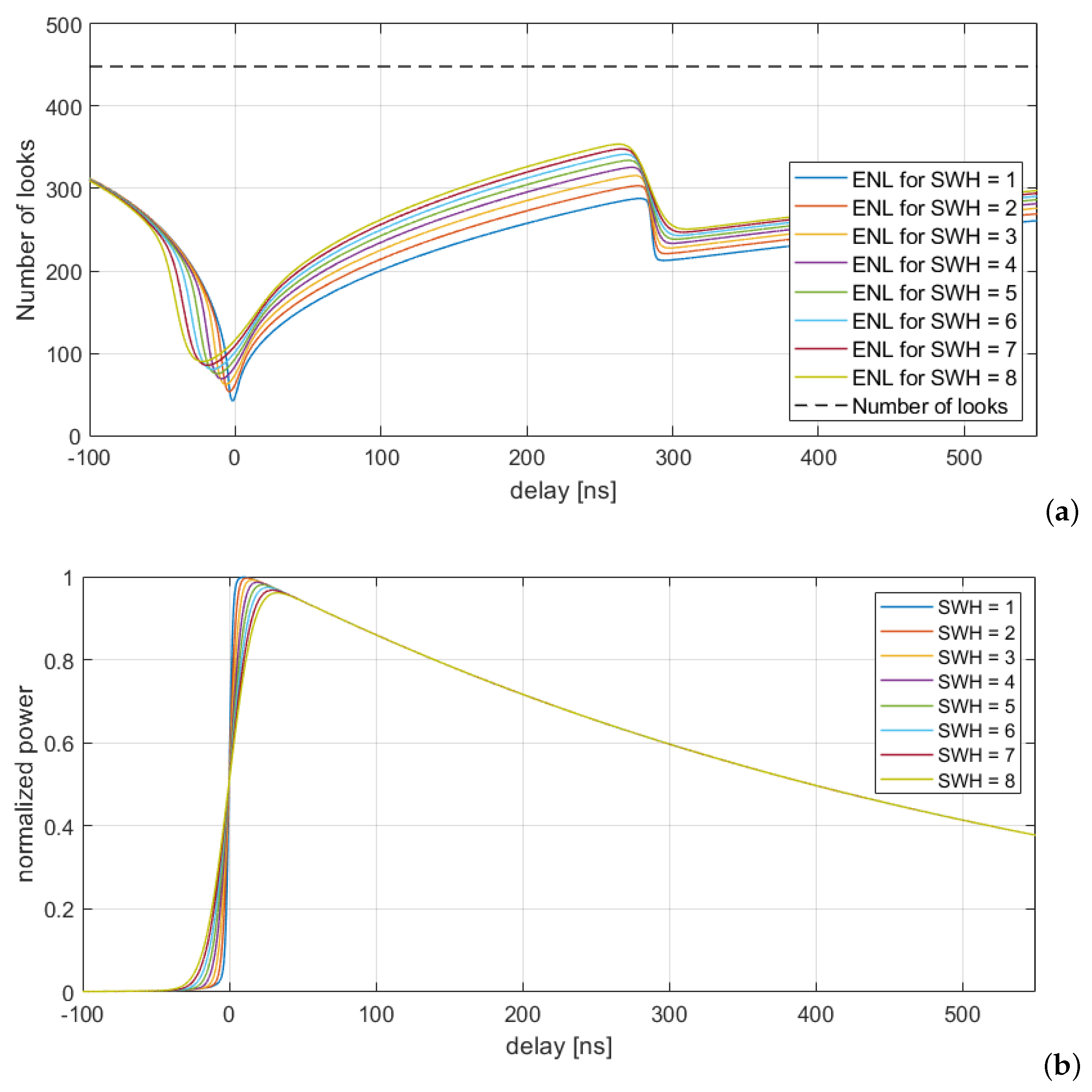
4.1. Theoretical ENL and Power Waveform
The power correlation function
R allows the evaluation of the theoretical ENL according to Equation (
6). To this aim, the along-track distance of each pair of pulses to be included in the multilooking are selected according to the instrument chronogram, i.e., the displacement in the along-track direction of the satellite between each pair of pulses is computed according to the PRF and satellite velocity. The assumption is to have a homogeneous wave height condition in the extent of the multilooking time.
Figure 2a shows the theoretical ENL for different wave heights for S6-MF LR mode echoes, obtained by averaging all the available pulses in a tracking cycle. For comparison, the number of averaged echoes, representing the upper bound for the ENL, is plotted as a dashed line on the top. This ENL value would be obtained only in the case of complete decorrelation of the averaged echoes.
Figure 2b shows the pulse-limited power waveforms obtained with S6-MF parameters and the same range of SWH values. This plot provides a correspondence between the ENL trend and the power waveforms trend in the different areas: the thermal noise area, the leading edge, and the trailing edge.
As can be seen from
Figure 2a, an increasing SWH produces an overall enhancement of the ENL, due to the progressive decorrelation of the averaged pulses. Moreover, for all the SWH values, the resulting ENL shows an extremely variable dynamics along the delay time dimension, with the lowest value achieved at the leading edge and higher values obtained at the waveform trailing edge.
As expected, the continuous high-rate pulse mode of S6-MF provides an elevated number of highly correlated single looks, which translates to a ENL much smaller than the actual number of averaged values. This is also confirmed by the results in
Figure 2a.
4.2. Theoretical and Data-Based ENL in Subsampled Multilook
Considering the decrease in the pulse-to-pulse correlation for larger values of along-track distances, an alternative multilooking method is considered, consisting of averaging a lower number of waveforms by an integer decimation, so as to reduce the correlation among successive waveforms. Different decimation factor can be used.
Figure 3 shows the theoretical ENL (solid lines) obtained from different incoherent averaging decimation strategies and for two different values of SWH. Two decimation strategies were used:
Taking one pulse out of two, leading to an equivalent acquisition frequency of ∼4.5 KHz;
Taking one pulse out of five, leading to an equivalent acquisition frequency of ∼1.8 KHz close to the Walsh limit.
As expected, for the considered multilooking methods, the ENL is lower than the one obtained for the 9 KHz case, but it is much closer to the actual number of averaged echoes, addressed by the dashed line of the corresponding color.
As limit, for the 1.8 KHz case, the ENL is almost coincident with the number of averaged echoes, as expected from the decorrelation of the single-look pulses. Moreover, the ENL in correspondence of the leading edge (i.e., delays close to 0) is very similar for all three cases, while the greatest differences are observed in the trailing edge region.
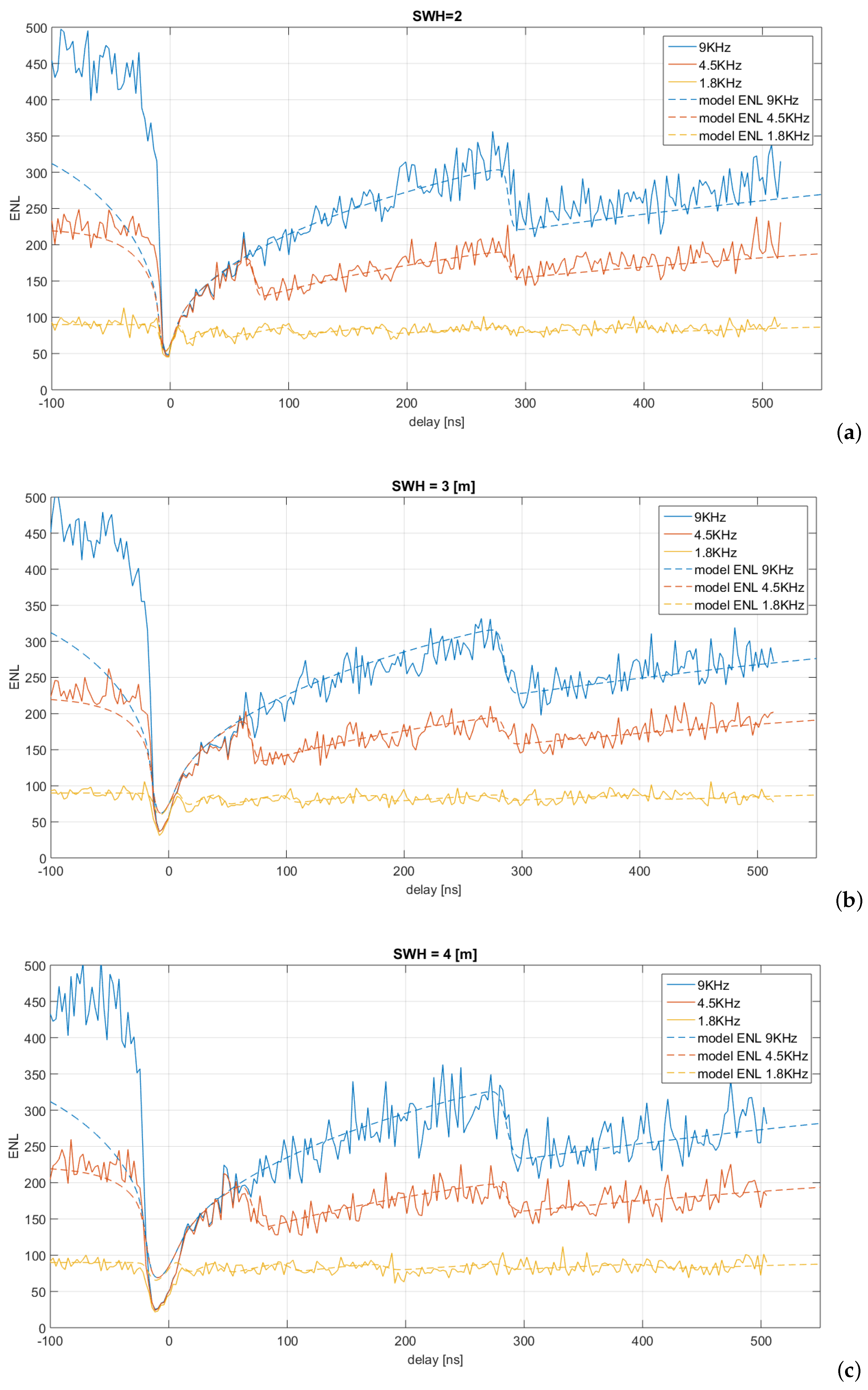
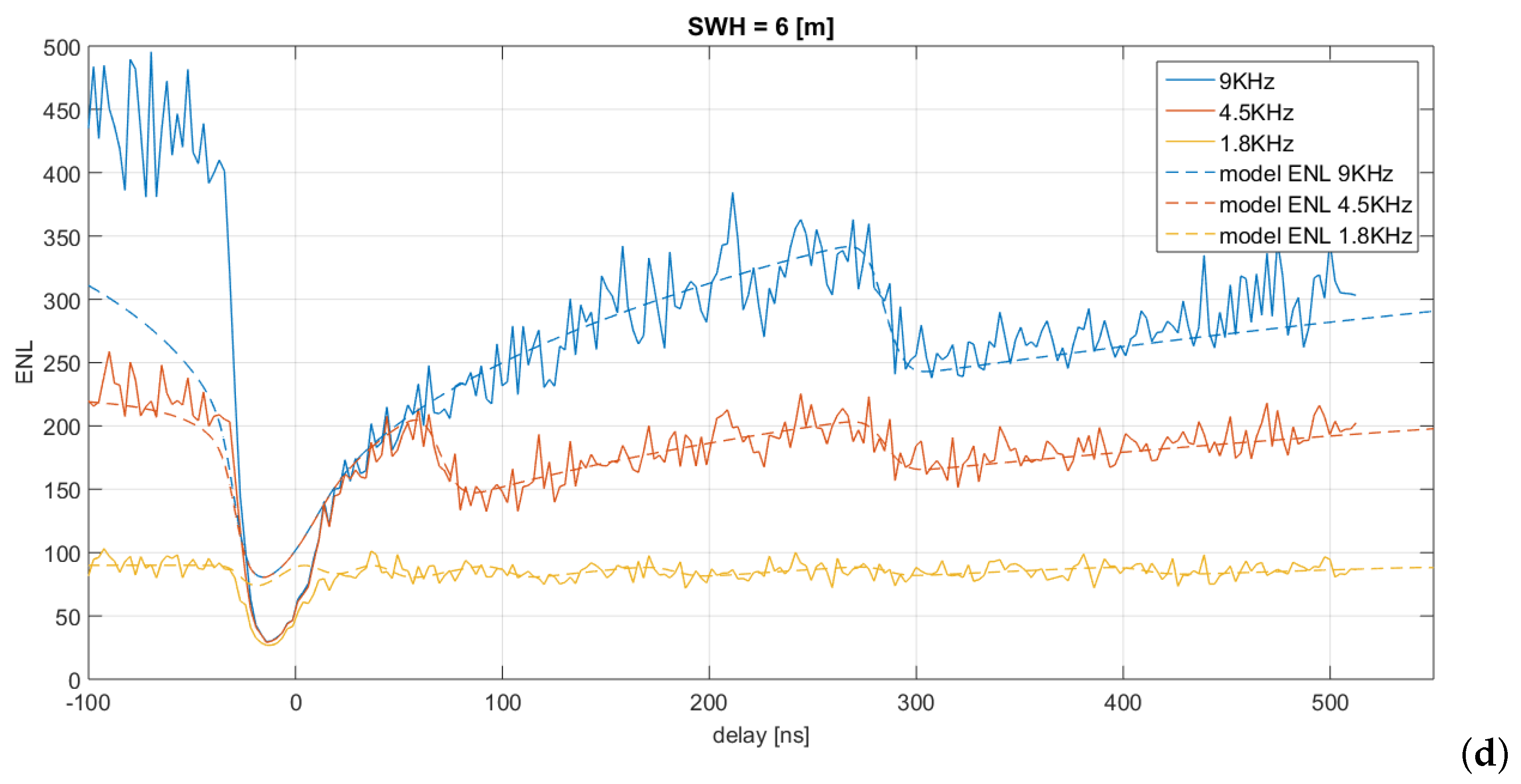
The theoretical plots were replicated using true data from S6-MF cycle 9 data over open ocean. L1A were bprocessed with different decimation factors, and a retracker based on the model in [
15] was applied to estimate the SWH values. Finally, portions of data with omogeneous SWH values were used to obtain an empirical estimation of the ENL for different sea wave heights. In
Figure 4, the ENL is shown for different values of SWH and
as decimation factors. The corresponding dashed lines represent the averaged number of echoes.
The ENL retrieved from data are in line with the theoretical result, although some points need to be discussed.
First, the different behavior of the leading edge at various SWH (see
Figure 2b) is explained by the increasing of azimuthal dispersion, which generates a larger bandwidth. This produces a faster pulse-to-pulse decorrelation and the blunter shape of the leading edge waveform. Part of the energy of the leading edge, then, leaks into the noise area.
For the noise area, in both theoretical and data-based plots, it would be expected that ENL in the noise area were equal to the number of looks averaged (see
Figure 3 and
Figure 4) due to the decorrelation introduced by the thermal noise. Instead, an asymptotic trend towards such value is seen. This behavior is just due to the leakage of the leading edge energy mentioned before. Due to this leakage, the waveform results partially correlated also in the noise area, at least in proximity of the leading edge. As SWH increases, due to the blunter leading edge shape, the asymptotic value (i.e., the theoretical ENL) is reached slower. Moreover, since the theoretical curves, as in
Figure 3, do not include the noise, the real number of looks in the noise area is higher (due to the presence of the noise, that decorrelates), as can be seen when comparing the solid and dotted lines in
Figure 4.
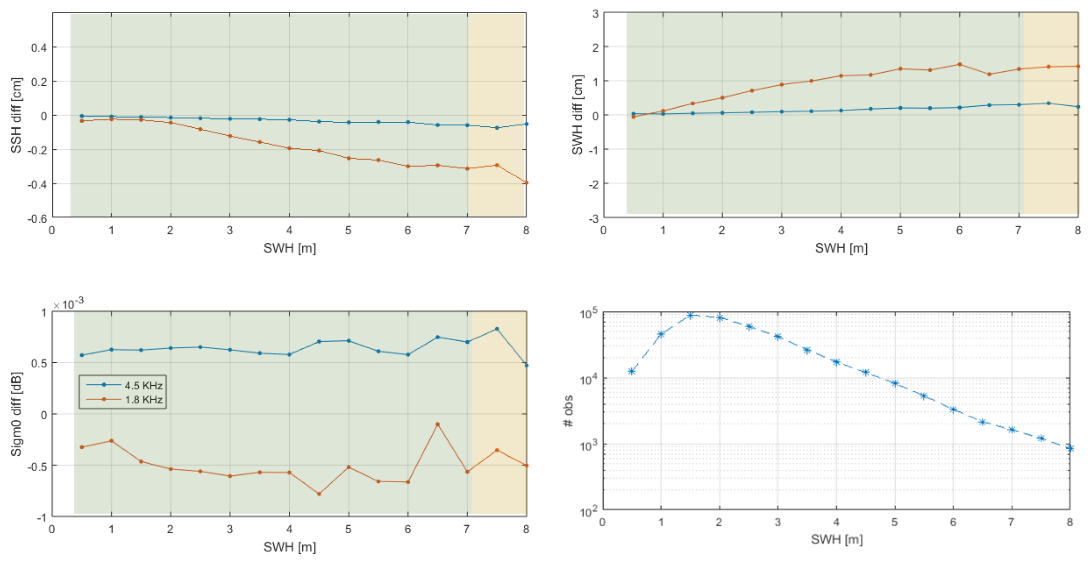
4.3. Geophysical Parameters Estimation
The
, the sea surface height (SSH), and the significant wave height were retrieved from all the 256 S6-MF L1A pole-to-pole passes from cycle 9 and processed with the three different decimation factors considered in the previous section by making use of a geophysical retracker based on the model in [
15].
Bias. It is known that the use of high PRF in acquisition introduces a bias in the estimate of the geophysical parameters [
12,
17]. Differently from that reported in the cited papers, this bias was evaluated using the original S6-MF PRF as reference and evaluating the difference in accuracy in case of a decimation equal to 2 and 5, the last corresponding to an acquisition of about
kHz. In
Figure 5, the SSH, SWH, and
are reported. It is worth noticing that the estimated bias is on the order of few centimeters for SWH and below 0.4 cm for SSH. As expected, the bias is more pronounced with respect to the ≈1.8 kHz case (red lines) and slightly increases with the SWH. For
, the biases are below
dB and do not show a dependence on SWH.
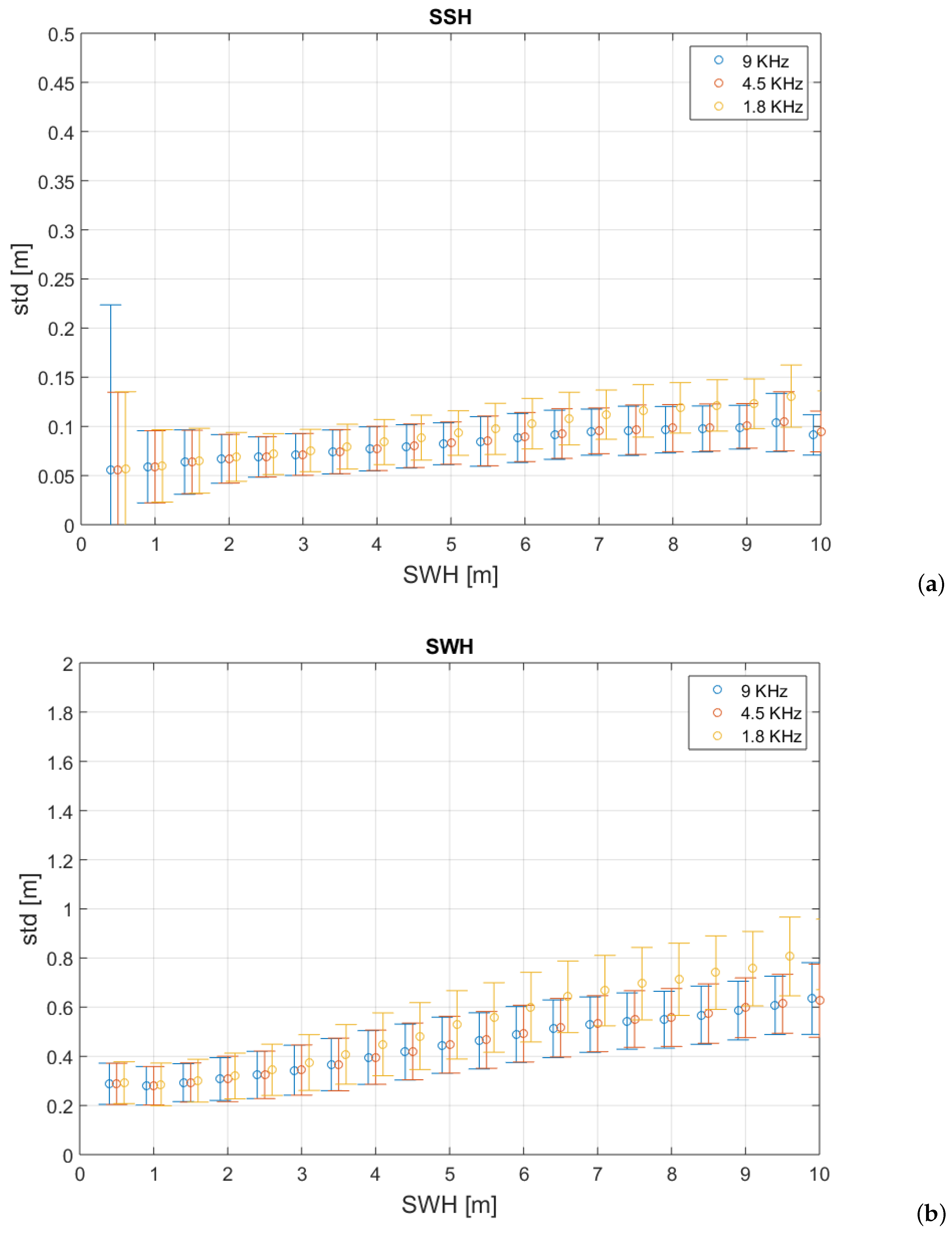
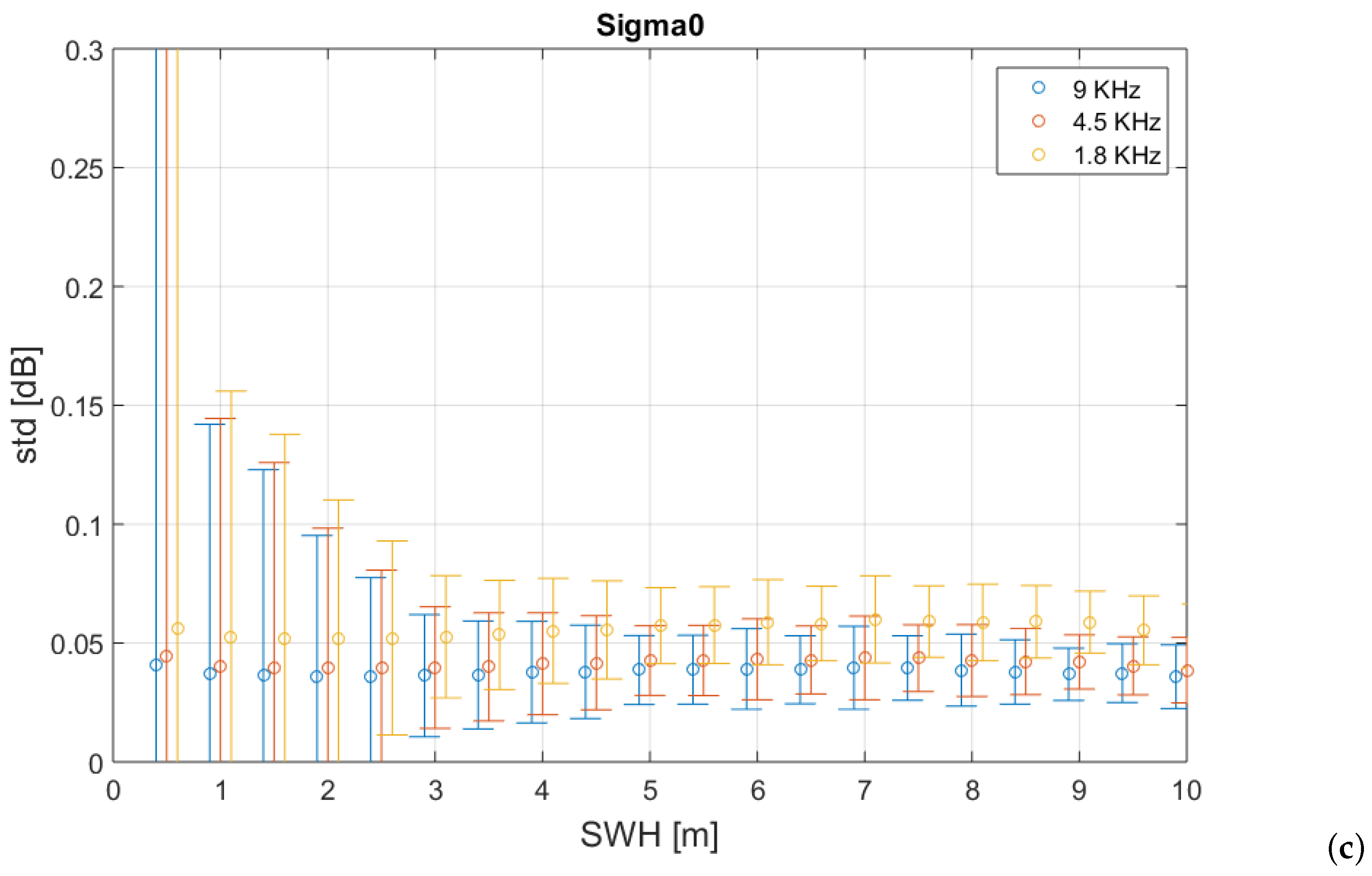
Precision. In
Figure 6, the
, the SSH and the SWH precision (i.e., standard deviation) is shown as a function of the
. The dispersion of the sample standard deviation is addressed by the error bar around the estimated value, indicated by the circle and is a function of the number of observations. While the precision of
is basically unvaried with
, we see a decrease of the precision (i.e., the standard deviation increases) as
increases, for both
and
, regardless of the decimation factor used. This is addressed by the increasing trend of the circles with the
.
The partial correlation of the waveforms at high PRF has basically minimal or null effects on
and
precision, at least for low values of
. This means that the standard deviation is basically the same for low
, regardless of the decimation factor (represented by the different colors in
Figure 6).
5. Discussion
The autocorrelation function properties were widely explained in [
12]. The behavior at the leading and trailing edges was interpreted in terms of waveform correlation (in the leading edge) and successive decorrelation (in the trailing edge), resorting to the van Cittert–Zernike theorem [
18]. Here, the function was retrieved from real S6 data and for two different ocean conditions (SWH), with results in agreement with previous literature (compare
Figure 3 and
Figure 4 with
Figure 3 of [
12]).
The observed decorrelation with the along-track distance with high
is expected: in fact, for higher SWH, portions of the sea surface contributing to the energy in the late-range bins are spread more broadly in the along-track distance. According to the van Cittert–Zernike theorem, this results in a broader Doppler bandwidth and in a faster decorrelation with along-track distance [
12].
The theoretical ENL retrieved for increasing values of shows that the leading edge is the most correlated part (ENL is low), and this is almost invariant with the ; instead, in the thermal noise area, the value is quite close to the maximum attainable (about 448 with S6-MF parameters, corresponding to the total number of pulses in a radar cycle that are averaged to generate a single LR pulse) since the thermal noise can be assimilated to a white noise, which decorrelates faster than the PRI interval.
This signal-free area is reduced, however, by the energy leakage from the leading edge of the waveform, resulting in a mixed area of thermal noise and physical signals with lower ENL values. The leaking is slightly different for different
, due to the shape of the leading edge, which is sharper for low
and blunter for high
[
15]. This means that for high
more energy is leaked in the thermal noise area, and this reflects in a lower value of ENL in the mixed area as
increases.
The ENL was evaluated using different PRF, just by using different integer decimations of the waveforms. As expected, a higher sampling frequency provides a higher ENL (see
Figure 4).
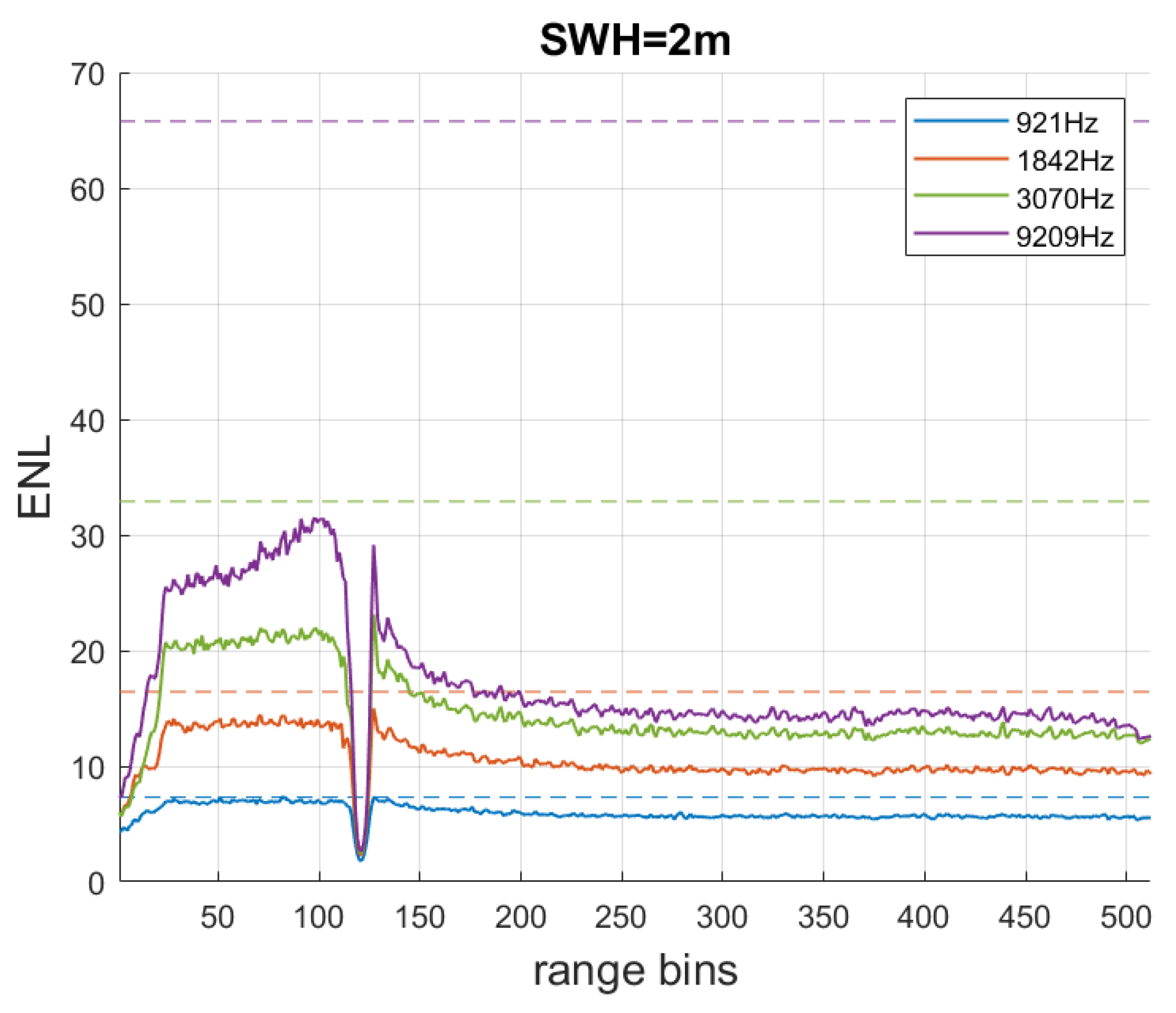
The high sampling frequency of acquisition has opened the possibility to obtain multilooked data at a posting rate higher than 20 Hz (typical of LRM products). This means we can obtain geophysical parameters at a higher rate with comparable accuracy with the ones in LRM products. Full-focusing processing becomes, then, fundamental to overcome the LRM products for future missions such as CRISTAL. In a preliminary result, an open ocean dataset with
m was fully focusing processed and then multilooked at a posting rate of 140 Hz. The ENL profiles with the slant range are shown for different decimation factors in
Figure 7. The trend of ENL with slant range is slightly different from the one achieved in the LRM case. A proper theoretical formulation and an in-depth analysis is then necessary in future work.
6. Conclusions
In this paper, the theoretical and data-based autocorrelation function of the S6-MF pulse waveforms were investigated.
The ENL was evaluated from theory and compared with the same quantity estimated using open ocean datasets in different ocean conditions, showing a high degree of agreement. The ENL was estimated in different decimation cases with respect to the original S6 PRF. The plots confirmed that the high sampling rate acquisition system gains an equivalent number of looks. However, the partially correlated waveforms produce a bias with respect to the optimal sampling step, supposed at the Walsh bound.
It is important to point out here that the increase in the PRF improves the precision of the geophysical parameters, thanks to more looks available, but introduces estimation biases. These biases could be corrected empirically using a look-up table or more elegantly and properly handled by using a maximum likelihood estimator (MLE). This is crucial for the S6-MF mission, for having objectives to provide, such as reference mission and highly accurate time series of sea level measurements.


