A Comparative Study on Multi-Parameter Ionospheric Disturbances Associated with the 2015 Mw 7.5 and 2023 Mw 6.3 Earthquakes in Afghanistan

Abstract

This paper presents a multi-parameter ionospheric disturbance analysis of the total electron content (TEC), density (Ne), temperature (Te), and critical frequency foF2 variations preceding two significant earthquake events (2015 Mw 7.5 and 2023 Mw 6.3) that occurred in Afghanistan. The analysis from various ground stations and low-Earth-orbit satellite measurements involved employing the sliding interquartile method to process TEC data of Global Ionospheric Maps (GIMs), comparing revisit trajectories to identify anomalies in Ne and Te from Swarm satellites, applying machine learning-based envelope estimation for GPS-derived TEC measurements, utilizing the least square method for foF2 data and ionograms obtained from available base stations in the Global Ionosphere Radio Observatory (GIRO). After excluding potential influences caused by solar and geomagnetic activities, the following phenomena were revealed: (1) The GIM-TEC variations displayed positive anomalies one day before the 2015 Mw 7.5 earthquake, while significant positive anomalies occurred on the shock days (7, 11, and 15) of the 2023 Mw 6.3 earthquake; (2) the Swarm satellite observations (Ne and Te) for the two earthquakes followed almost the same appearance rates as GIM-TEC, and a negative correlation between the Ne and Te values was found, with clearer appearance at night; (3) there were prominent positive TEC anomalies 8 days and almost 3 h before the earthquakes at selected GPS stations, which were nearest to the earthquake preparation area. The anomalous variations in TEC height and plasma density were verified by analyzing the foF2, which confirmed the ionospheric perturbations. Unusual ionospheric disturbances indicate imminent pre-seismic events, which provides the potential opportunity to provide aid for earthquake prediction and natural hazard risk management in Afghanistan and nearby regions.

1. Introduction

Ionospheric sounding is a technique for investigating the behavior and properties of the ionosphere, a component of the Earth’s upper atmosphere. Ionospheric disturbances are becoming recognized as potential predictors of seismic activity as significant disturbances have been widely observed by various techniques before the occurrence of earthquakes [1,2,3]. During pre-earthquake stages, the Earth’s energy balance is disrupted due to the release and emission of thermal energy [4,5], or gases such as radon, caused by fault activation [6]. Disturbances in the lithosphere move across the geospheres (lithosphere, cover sphere, atmosphere, and ionosphere), leading to traveling anomalies in each sphere [7].

The particular mechanics causing the electric discharges are not well understood, and several theories have been proposed to explain their occurrence, such as them occurring before an earthquake due to increased stress and strain in the active fault zone, causing rocks to generate a rise in electric discharges through a phenomenon called piezoelectricity. Piezoelectricity occurs at the atomic level when ions are displaced within a soil or rock’s crystal lattice as a result of stress. This displacement induces an imbalance of electric charges, which generates a voltage across the material [8]. One concept proposes that stress-induced electrical charges within rocks, known as p-holes, have the capacity to accumulate. As p-holes from the earthquake’s hypocenter gather on the ground surface, they can alter the Earth’s electromagnetic field and ionize air molecules at the ground–atmosphere interface. This ionization process can produce a variety of abnormal occurrences in the atmosphere and ionosphere [9,10]. When the tension reaches a critical level, the stored charge is suddenly released, resulting in an electric discharge that alters the near-surface atmospheric electric field [11]. Additionally, the build-up of p-holes on the surface is thought to lower the microwave dielectric constant of the ground and increase regional microwave radiation [12,13]. An alternative theory posits that the mechanical fragmentation of rocks during seismic activity, coupled with the release of radon gas previously trapped within the soil and crust, can lead to a series of seismic anomalies. The decay of radon gas contributes to the ionization of the surrounding air, thereby inducing various abnormal perturbations in aerosol concentration, atmospheric humidity, latent heat, and ionospheric plasma. Seismic-related abnormalities in radon emission can be linked to pre-seismic electromagnetic phenomena, such as substantial changes in ion concentration and the atmospheric electric field [14]. These alterations in the atmospheric and ionospheric conditions facilitate the formation of charged aerosols, which in turn play a role in the generation of electric discharges during seismic events [15].

Recent studies have highlighted the growing efficiency of observational techniques in detecting ionospheric disturbances associated with earthquakes using advanced machine learning models, such as autoregressive integrated moving average (ARIMA), long short-term memory (LSTM), the nonlinear autoregressive network with exogenous inputs (NARX) model, and remote sensing techniques [16,17]. These techniques include the use of various tools such as the Global Navigation Satellite System (GNSS) [18] and electromagnetic satellites [19,20]. Scientists have adopted hybrid machine learning approaches for TEC predictions, demonstrating the compatibility of deep learning in dealing with complex ionospheric data [21,22,23]. Notably, the effectiveness of LSTM approaches has been demonstrated to predict TEC values with a time of 24 h [24]. Deep learning methods can be applied to construct the TEC reference background, thus contributing to a better extraction of ionosphere disturbances.

Over the past few decades, numerous studies have demonstrated a direct or indirect relation between the occurrences of geohazards and ionospheric disturbances. He and Wu advocated one-to-one correspondence between ionospheric anomalies and large earthquakes using integrated wavelet analysis [25,26]. Pulinets, Iwata, and Kandalyan discovered that ionospheric abnormalities, identified using a variety of ionospheric sounding techniques, can serve as reliable precursors to earthquakes [27,28,29]. Xu reported unusual variation in the ionospheric F-region critical frequency prior to the Wenchuan earthquake, underlining the potential of ionospheric sounding for pre-earthquake identification [30]. Xie at al. adopted multi-sensor analysis for ionospheric electron content and density determination [20]. Notably, regarding ionospheric plasma disturbances, Parrot et al. observed a significant increase in electron density (Ne) over the Kii Peninsula a full week prior to the earthquake [31]. Marchetti and Akhoondzadeh proposed the creation of a Swarm data-based ionospheric monitoring network as an earthquake early-warning system to assess the strong (Mw = 8.2) earthquake that struck Mexico on 7 September 2017 [32]. Liu et al. observed that foF2 anomalies increased with earthquake magnitude but decreased with distance from the ionosonde station to the epicenter for Taiwan’s 184 earthquakes (Mw > 5.0) from 1994 to 1999 [33]. Cherrier et al. introduced a TEC time series forecasting model based on LSTM networks. Their findings confirmed the promising capabilities of LSTM in accurately predicting time series data [34]. Salikhov used the Doppler sounding technique, employing the continuous monitoring of the Doppler frequency shift of reflected radio signals to investigate the ionosphere above earthquake sources [35]. Thereafter, Sharma, Tachema and Nayak investigated and supported the correlation between seismic activity and ionospheric anomalies through the analysis of total electron content (TEC) fluctuations, and crustal stress (b-value) precursors to identify potential precursors and assess their effectiveness in short-term seismic prediction for the 2010 Mw 7.2 Mexico earthquake, the 2011 Mw 5.1 Lorca earthquake in Spain, and the 2022 Mw 7.7 Colima earthquake in Mexico [36,37,38].

In contrast to previously conducted studies on multi-parameter anomaly detection methods for seismic ionosphere disturbance [26,39,40], this study distinguishes itself in numerous significant ways. Firstly, it takes a comprehensive approach by combining multi-parameter anomaly detection algorithms, allowing for a more effective study of earthquake instances with an emphasis on temporally collocated ionospheric disturbances. Second, a simultaneous multi-platform approach is used, which includes a thorough examination of parameters such as TEC from GIMs along with ground-based GNSS stations, electron density, and temperature from Swarm satellites, as well as ionospheric height and critical frequency from ionosonde base stations. Additionally, the results collected from Swarm satellites are confirmed using ionograms. Finally, this study analyzes recent, severe, and unaddressed earthquake cases in Afghanistan, with the goal of finding the underlying geophysical phenomena that lead to earthquake hazards.

By exploring these aspects, this study has the potential to provide valuable insights for earthquake prediction and contribute to the management of natural hazard risks in Afghanistan and neighboring regions. The integration of data from multiple platforms allows for complementary and mutually reinforcing verification at different spatiotemporal scales, enabling the precise identification of ionospheric anomalies. Involving the integrated use of GNSS, electromagnetic satellites, advanced machine learning techniques, and multi-parameter analysis aims to improve the detection, analysis, and prediction of ionospheric disturbances associated with earthquakes. Moreover, in this analysis, the cross-verification of TEC from multiple data sources such as IONOLAB and SIMRug is considered to be a necessity to exclude true anomalies [41,42]. These advancements contribute to a more comprehensive and correct understanding of ionospheric disturbances as potential earthquake precursors.

2. Data and Methods

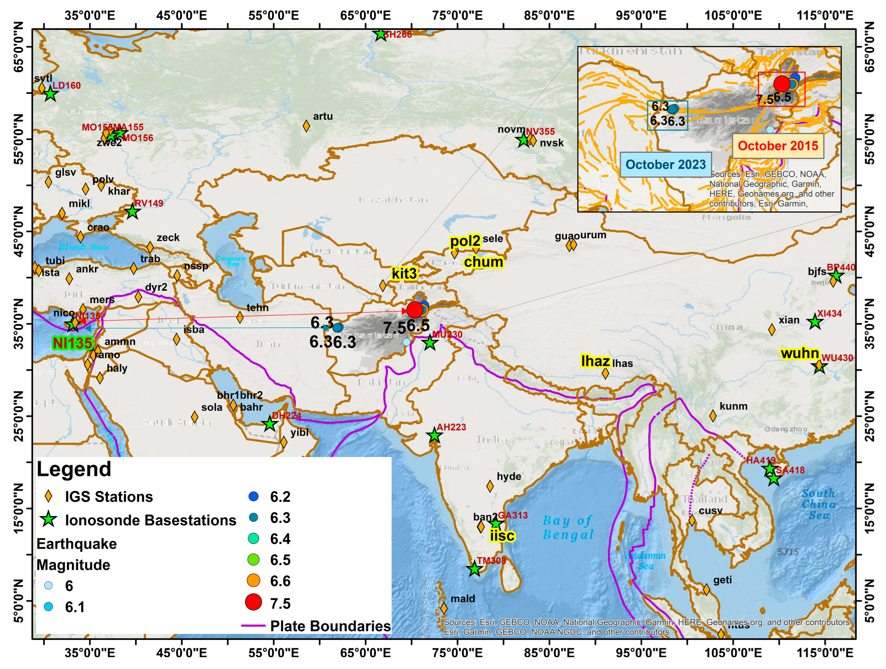
2.1. Tectonic Setting of Afghanistan Earthquakes

The 800 km long Hindukush Range in Afghanistan is part of a collision zone between the Eurasian and Indian tectonic plates, incorporating several active faults such as the Chaman fault system and Kabul fault system; it has high potential to generate earthquakes. For this reason, the earthquake cases studied are as follows.

A 7.5 magnitude earthquake struck northeast Afghanistan (36.5244°N, 70.3676°E) on 26 October 2015. The quake occurred at an intermediate depth of 210 km due to reverse faulting [43].

Between 7 and 15 October 2023, a series of earthquakes and aftershocks struck Herat Province in western Afghanistan, killing 1482 people, injuring 2100, and damaging 3330 dwellings. The aftershocks lasted until 28 October 2023. On 7 October 2023, an earthquake with a magnitude of 6.3 struck 32 km from Qarabag, 34 km from Zendijan, and 41 km from Gurian in Herat, Afghanistan. The event occurred at 34.5982°N and 61.9263°E at a depth of 14 km. On 11 October 2023, a 6.3 magnitude earthquake struck 28 km north of Herat city in Herat Province, western Afghanistan, at 34.5364°N and 62.0509°E. On 15 October 2023, another 6.3 magnitude earthquake struck 34 km north of Herat city in Herat Province, western Afghanistan, at 34.6529°N and 62.1244°E [44].

The earthquake cases selected in the research were acquired from the United States Geological Survey (USGS) (https://earthquake.usgs.gov/earthquakes/search/, accessed on 1 January 2024). This research focuses on studying primary shocks within earthquake clusters in Afghanistan’s active fault zones (Figure 1) in order to reduce risks, improve the understanding of earthquake dynamics, and develop effective seismic mitigation measures.

2.2. Spatiotemporal Data Selection Criteria

To detect reliable abnormalities in the ionosphere caused by seismic activity, Wu et al. developed a Deviation–Space–Time (DST) criterion, which was also used in this study for analysis and validation [45]. The DST criterion is made up of three components: first, the observed parameter deviates significantly from its expected values, indicating its potential as an anomaly; second, the occurrence of multiple anomalies exhibits quasi-synchronous behavior in time; and third, the reported anomalies are spatially contiguous, indicating geographic adjacency. This DST criterion is used to detect and investigate ionosphere anomalies connected with seismic occurrences while limiting false positives [46]. Large magnitudes have a significant impact on ionospheric disturbances. To ensure compatibility, the size of the prepared seismic zone is computed using the formula (R = 10^0.43M), where R represents the radius in km and M indicates the magnitude [47].

2.3. Multi-Parameter Data and Processing

The complete route of ionospheric disturbances is well explained in Figure 2. GNSS data from ground-based Continuously Operating Reference Stations (CORSs), GIMs from the Center for Orbit Determination in Europe (CODE), foF2, hmF2, and ionograms from Digital Ionosonde Database (DID)—Global Ionosphere Radio Observatory (GIRO), and Ne and Te derived from Swarm satellite measurements were used to investigate ionospheric disturbances in Afghanistan from a perspective of multi-parameter analysis. GNSS stations within the Dobrovolsky distance of the epicenter were considered [47].

In the analysis of GPS data, a hybrid methodology involving machine learning, statistical analysis, and mathematical techniques was utilized. The 30 s interval TEC values were acquired from the available IGS databases of selected ground stations. GPS satellites transmit radio signals at two long-wavelength band frequencies: L1, which operates at 1.57542 GHz, and L2, which operates at 1.2276 GHz [37,38]. Satellite and receiver biases were removed, and Vertical TEC (VTEC) was derived from absolute STEC, which is measured in TECU (total electron content unit = 10¹⁶ e/m²). The STEC was calculated and converted into VTEC using GPS-TEC software v3.03. A hybrid machine learning algorithm, LSTM, was applied to train and predict the data over a 24 h period. By employing this machine learning-based envelope technique, a normal distribution of biased and unbiased VTEC values was opted for to establish a threshold of ±1.34 μ in order to achieve a higher level of confidence of almost 82% [48]. Any observed TEC values outside the range of ±1.34 µ signify the detection of abnormal signals [49]. Almost 10 GPS stations nearby the study area were processed, and those ground stations which were spatially closer to the epicenter, such as KIT3 (Uzbekistan), IISC (India), WUHN (China), LHAZ (China), CHUM (Kazakhstan), and POL2 (Kyrgyzstan), were considered for the actual anomaly estimation based on availability (see Table S2). This unique estimation method helped to accurately define abnormalities with the least data losses and RMS error rather than the historical methods of TEC anomaly estimations.

GIMs, generated by CODE, provide daily updates with a resolution of 5° longitude by 2.5° latitude, offering valuable insights into ionospheric conditions. To clearly identify the ionospheric anomalies, the sliding interquartile range (SIQR) method was used for GIM-TEC processing. The SIQR method utilizes data from CODE to identify TEC disturbances associated with earthquakes, establishing a baseline reference from pre-earthquake or stable periods and calculating the interquartile range (IQR) to determine abnormal ionospheric parameter values [33]. The IQR approach identifies anomalies that may not have a significant impact on the quartiles, ensuring a thorough examination. Data from individual GNSS receivers and GIM were used to account for both local and large-scale fluctuations. This technology increases the dependability and accuracy of our anomaly detection system, offering important insights into ionospheric anomalies and their potential relationship with seismic activity [50]. For calculating the interquartile range (see Equations (1) and (2)), the median of 2 consecutive days, i.e., Q₁, was subtracted from the 2-consecutive-day median of Q₃, and the upper and lower bounds were calculated by adding and subtracting the 1.4IQR from Q₂.

$${\mathrm{Q}}_1=\frac{{\mathrm{x}}_7+{\mathrm{x}}_8}{2},{\mathrm{Q}}_2=\frac{{\mathrm{x}}_{14}+{\mathrm{x}}_{15}}{2},{\mathrm{Q}}_3=\frac{{\mathrm{x}}_{21}+{\mathrm{x}}_{22}}{2}$$

(1)

$$\mathrm{I}\mathrm{Q}\mathrm{R}={\mathrm{Q}}_3-{\mathrm{Q}}_1, {\mathrm{x}}_{\mathrm{U}\mathrm{B}}={\mathrm{Q}}_2+1.4\mathrm{I}\mathrm{Q}\mathrm{R}, {\mathrm{x}}_{\mathrm{L}\mathrm{B}}={\mathrm{Q}}_2-1.4\mathrm{I}\mathrm{Q}\mathrm{R},$$

(2)

Seismic-related disturbances in TEC data can be identified by dividing the daily TEC values into overlapping time windows, calculating the IQR, and detecting deviations beyond a threshold, with Q₂ (the median) as a reference. x_UB and x_LB are the lower and upper bounds, respectively.

The ESA satellite mission of 3 Swarm (A, B, and C) low Earth orbit quasi-polar satellites was launched on 22 November 2013. Swarm B is at 520 km and A and C are at approximately 470 km; they are composed of specialized instruments, including a Langmuir probe, electric field instrument, absolute scalar magnetometer, and vector field magnetometer [51,52]. Ne and Te data from Swarm satellites A and C were downloaded from the IDP-IRR Level-2 daily Entire Mission data product for nearly three months. The Swarm Ne and Te data were analyzed using the revisit trajectory method. Trajectory data from three months before and five days after each earthquake were examined. Satellites A and C traveled through the epicenter at certain day and night times; for example, for the earthquake on 26 October 2023, the day and night revisit times were around 11 and 19 UTC, respectively, with an 8-day cycle. The data were categorized into two 2D groups and eight clusters based on access time, and background values from daytime and nighttime data were extracted for Ne and Te based on access time. When ΔNe and ΔTe values exceeded specified thresholds, as indicated by descending and ascending orbital–revisit plots, individual thresholds were calculated for Ne and Te during both day and night anomalies. Anomalies were defined as absolute values of ΔNe and ΔTe that exceeded 2σ (standard deviation of 2) [53]. The correlation between these aspects was analyzed to identify common patterns in the occurrence of anomalies.

An ionosonde radar system is also incorporated that probes the ionosphere by broadcasting radio signals at frequencies ranging from 0.1 to 30 MHz and receiving reflected signals from various ionospheric areas where the plasma frequency matches the radar frequency. In this work, the data utilized were gathered from the DID GIRO high-frequency pulse sounding system. This experimental configuration is focused on monitoring critical frequency (foF2) and F2-layer height (hmF2) at a specific geographic location approximately over the epicenters (latitude: 34°N, longitude: 62°E), for selected timescales (Figure S5). To assure accuracy, the data were calibrated using International Reference Ionosphere (IRI) models, which efficiently eliminated biases and reduced various types of noise. The system records, displays, and transmits vertical ionospheric data in the form of digital ionograms, accompanied by their associated parameters.

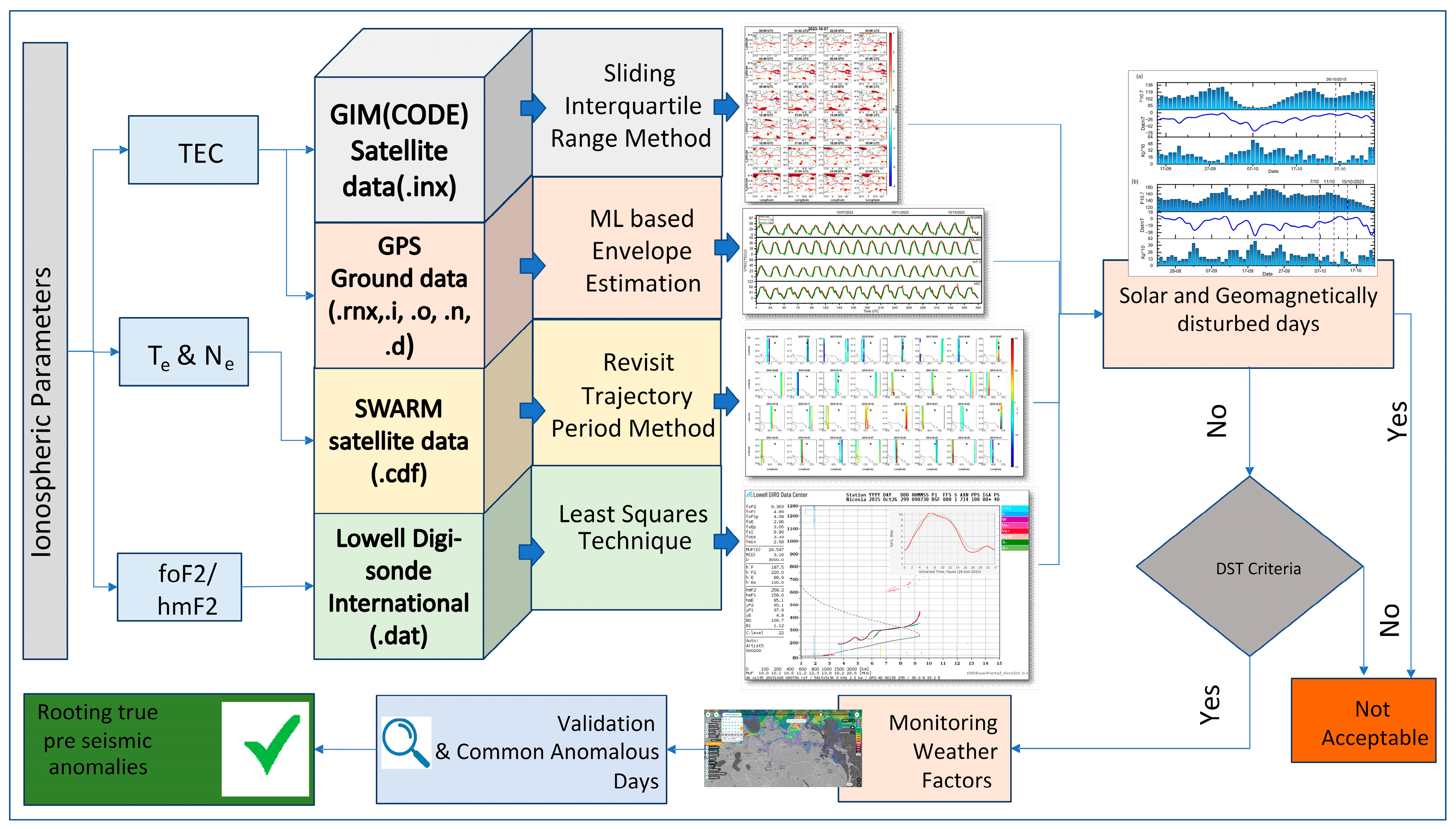
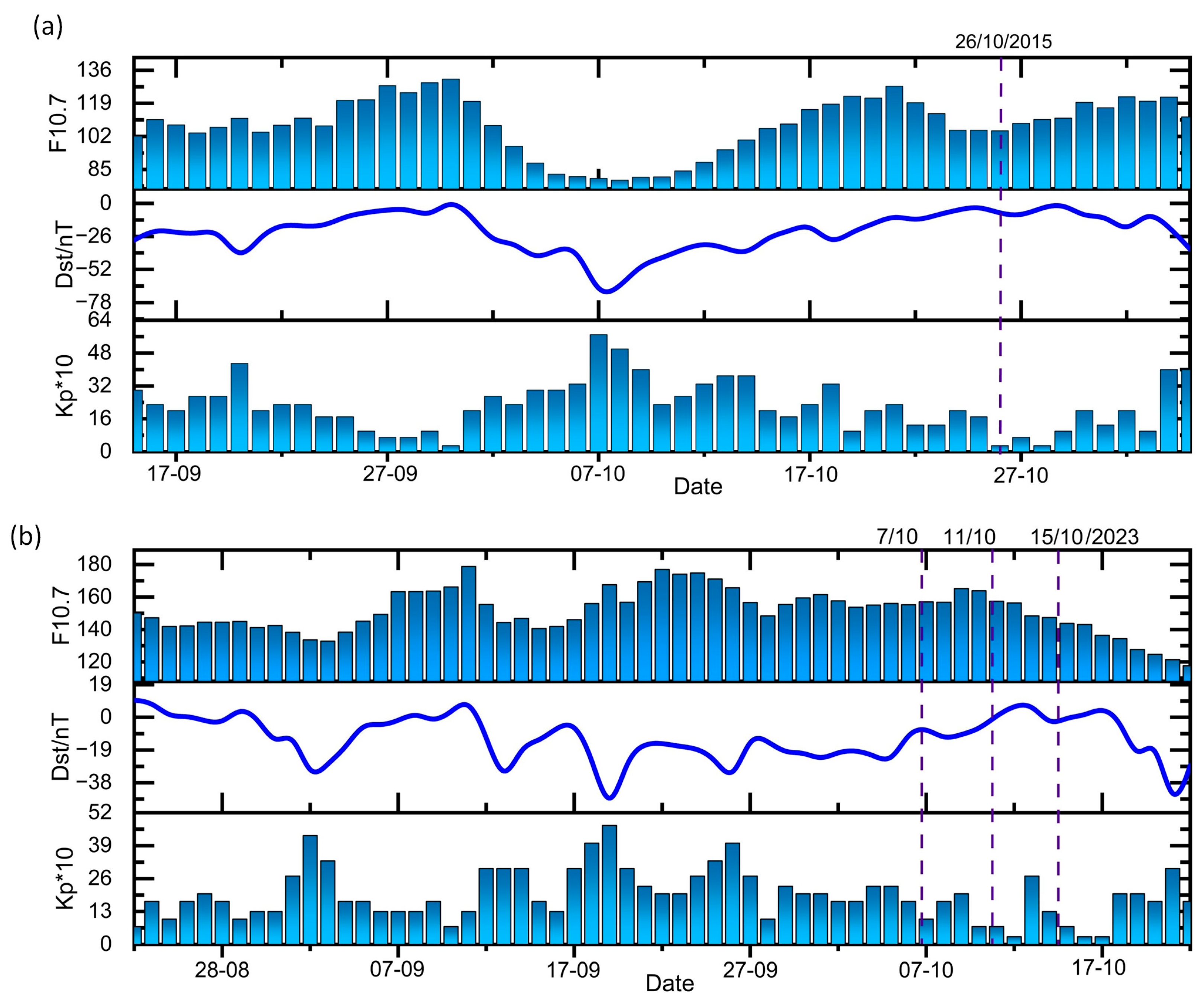
2.4. Solar–Geomagnetic Impact Exclusion

Solar and geomagnetic activities significantly impact the ionosphere, especially in equatorial and polar regions, making it challenging to differentiate between pre-seismic and solar–geomagnetic ionospheric phenomena [54]. To exclude potential influences associated with solar and geomagnetic activities, many indicators including Dst, Kp, and F10.7 were used in this study. Dst monitors equatorial ring current fluctuations (−200 to 200 nT), with negative values suggesting magnetic storms and positive values showing magnetic field recovery. The Kp×10 index (0–9) indicates overall magnetic conditions as measured at 13 Northern and 12 Southern Hemisphere stations. The F10.7 index monitors solar radio emissions (70 to 250 sfu), which represent solar activity levels. All daily averaged indices were obtained from OMNI Web (https://omniweb.gsfc.nasa.gov/form/dx1.html, Accessed on 18 January 2024). Geomagnetic weather (8–48 h) influences the global ionosphere, whereas seismic disturbances impact the ionosphere and are detected within 2000 km of the possible epicenter. Seismic–ionospheric disturbances occur three to four hours before an earthquake [15,55]. Table S1 and Figure 3 provide information on the exclusion of space weather disturbances. Disturbed days were identified based on criteria such as Dst > 30 nT, Kp×*10 > 40, and F10.7 > 130 Sfu. Figure 3a shows variations in these indices from 15 September to 5 November 2015, while Figure 3b displays variations from 15 August to 25 October 2023. Days affected by space weather disturbances were excluded from seismic disturbances by considering the presence of disturbances in GPS, GIM TEC, Te, or Ne data. If any of these parameters exhibited anomalies on a particular day, they were not considered a seismic disturbance. This approach ensured that only seismic-related anomalies were retained for analysis, enhancing the accuracy of the results.

3. Results

3.1. Multi-Parameter Ionospheric Anomalies

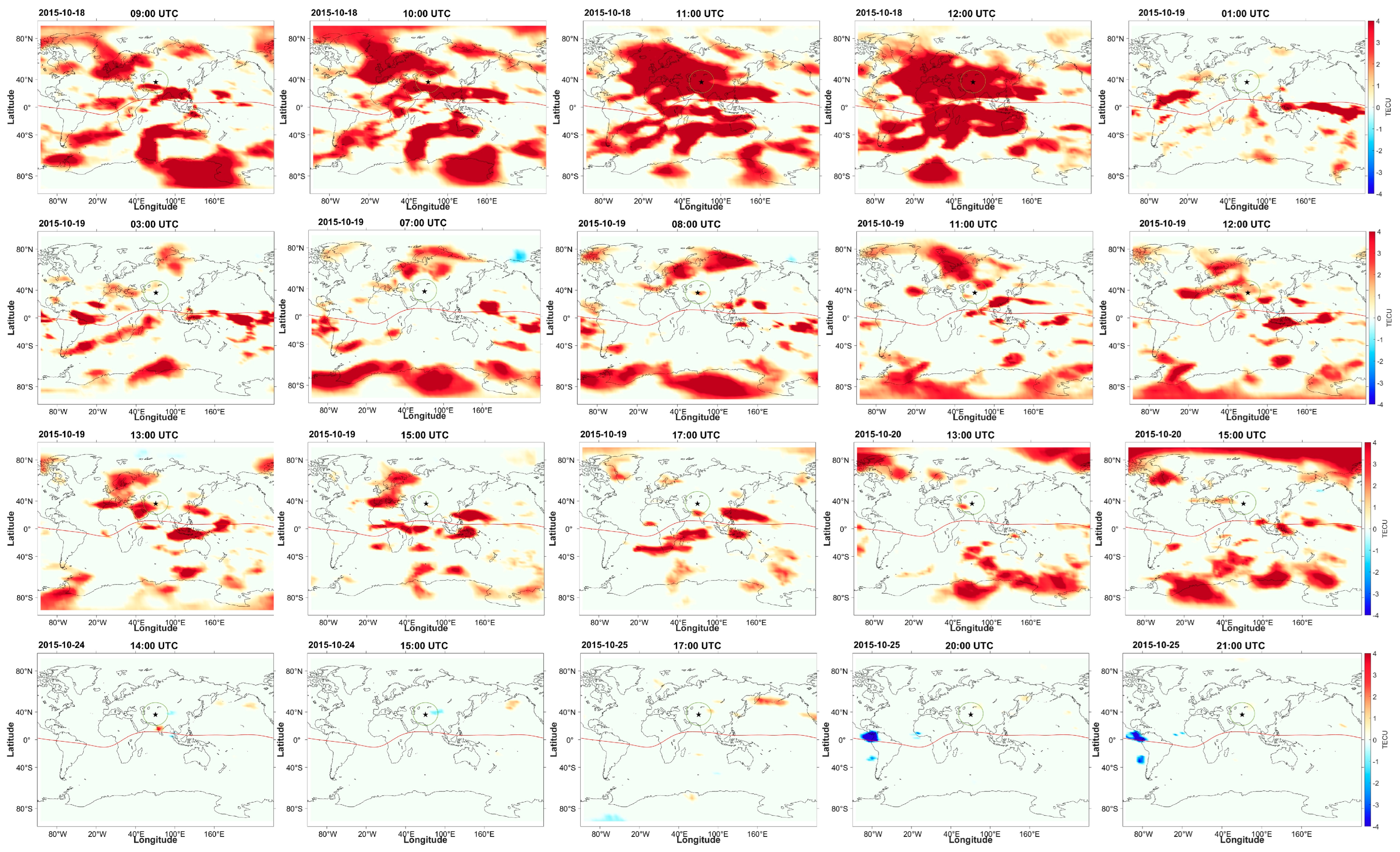
3.1.1. GIM-TEC Anomalies

The GIM-TEC data provide vital insights into the spatiotemporal distributions of ionospheric disturbances on a large scale. The detected abnormalities of GIM data were processed through the SIQR technique and are shown in Figure 4 and Figure 5 for both cases. After excluding the solar–geomagnetically disturbed days, the possible seismic ionosphere anomalies were as follows: the disturbances as positive and negative anomalies started appearing on 18, 19, 22, 24, 28, 29, and 30 September and 17, 18, 19, 20, 24, and 25 of October.

Exploring the days just before the earthquake, we observed minor negative disturbances around the northeast of the epicenter on 24 October 2015, while slight positive disturbances appeared on 25 October 2015. These disturbances serve as indications of pre-seismic activity. However, on 26 October 2015, no notable disturbances were observed. The spatiotemporal details can be seen in Figure 4.

Following the mitigation of anomalies arising from solar and geomagnetic disturbances, the residual irregularities within the dataset for the 2023 October earthquake are indicative of potential seismic ionospheric disruptions (see

Table 1. Common anomalies prior to the October 2015 earthquake; DOE is day of earthquake.

Date	GIM TEC Anomaly (@UTC)	GPS TEC Anomaly (@UTC)	SWARM Ne and Te Anomaly	Fof2 Anomaly Presence	Date	GIM TEC Anomaly (@UTC)	GPS TEC Anomaly (@UTC)	SWARM Ne and Te Anomaly	Fof2 Anomaly Presence
30-09-2015	9-11 (+)	-	(−) Ne Night/(+) Day\(−)Te Night/Day	-	19-10-2015	1-3, 7-9, 11-13, 17-19 (+)	13-16 (+)	(+) Ne Day\Te Day (+)	✓
03-10-2015	15-17 (−)	-	(−) Ne Night\(+) Te Night	-	20-10-2015	13-15 (SW of epicenter) (+)	12-14 (+)	(+) Ne Day\Te Day (+)	✓
15-10-2015	9-12 (+)	8-12 (+)	(+) Ne Night/Day\Te Night (−)	-	24-10-2015	13, 15 East of epicenter (−)	16-19 (+)	(+) Ne Night\Te Night (−)\Te Day (+)	✓
17-10-2015	8-19 (+)	6-9 (+)	(+) Ne Day\Te Night (−)	✓	25-10-2015	20, 21 (NE of epicenter) minors (+)	15-18 (+)	(+) Ne Night\Te Night (−)\Te Day (+)	✓
18-10-2015	9-13 (+)	11-18 (+)	(+) Ne Day\Te Day (+)	✓	26-10-2015 (DOE)	-	6-8 (+)	(+) Ne Night/Te Night/Day (−)	✓

). Notably, pre-earthquake anomalies manifested on multiple dates, starting from 9, 12, 14, 21, 24, and 30 September, as well as 1, 2, 3, 6, 7, 9, 10, 11, 13, 14, and 15 October 2023.

The anomalies started appearing 28 days before the earthquake; the nearest anomaly witnessed before the earthquake occurred on 6 October 2023 at 14:25 UTC, which was only 7–5 h before, and that for the first earthquake that occurred on 7 October 2023 at 07:12 UTC was seen 5–3 h before the impending earthquake, as shown in Figure 5. The 24 h anomaly appearances for all mentioned days are provided in Supplementary Materials Figures S1 and S2 for both cases.

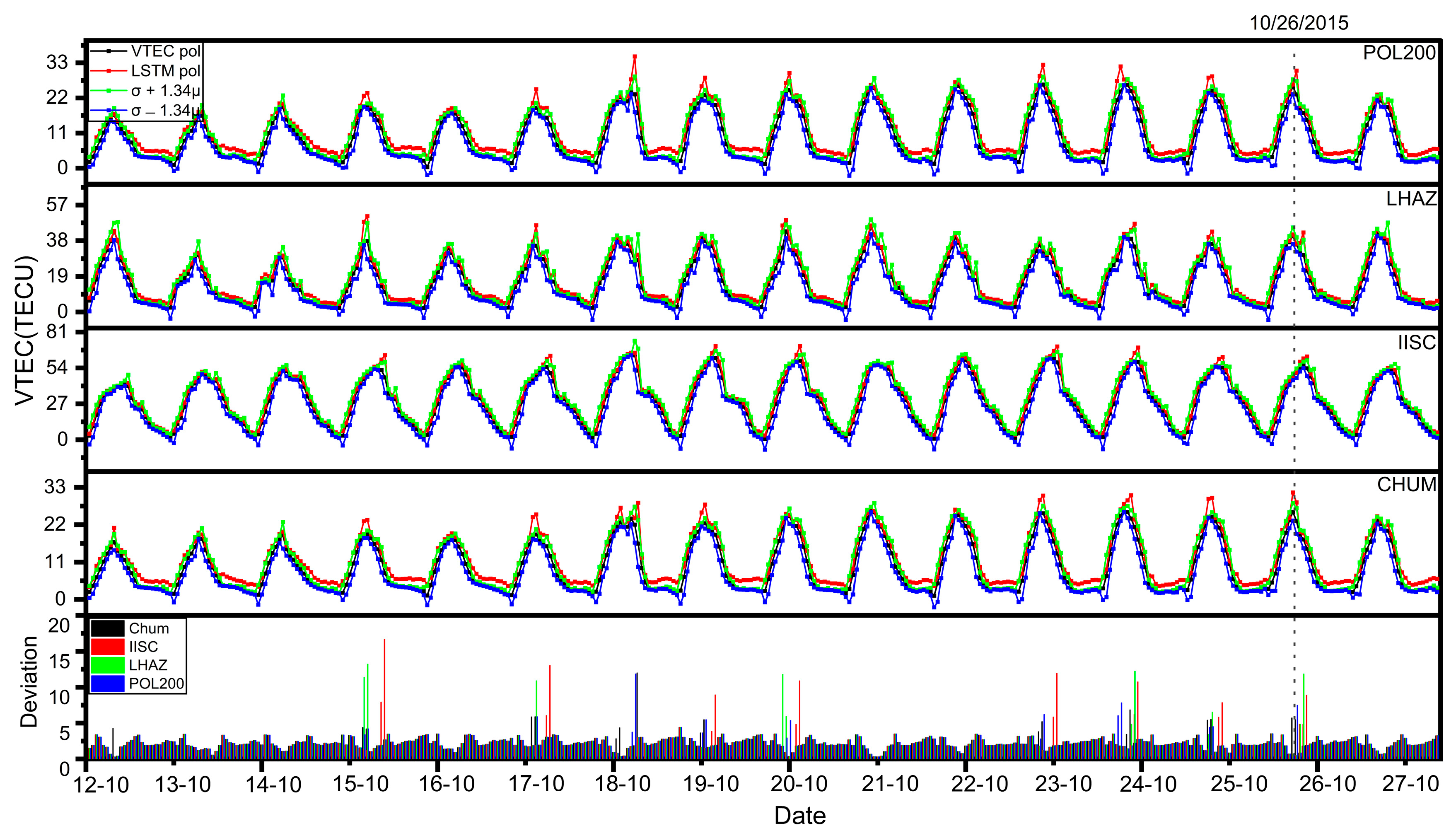
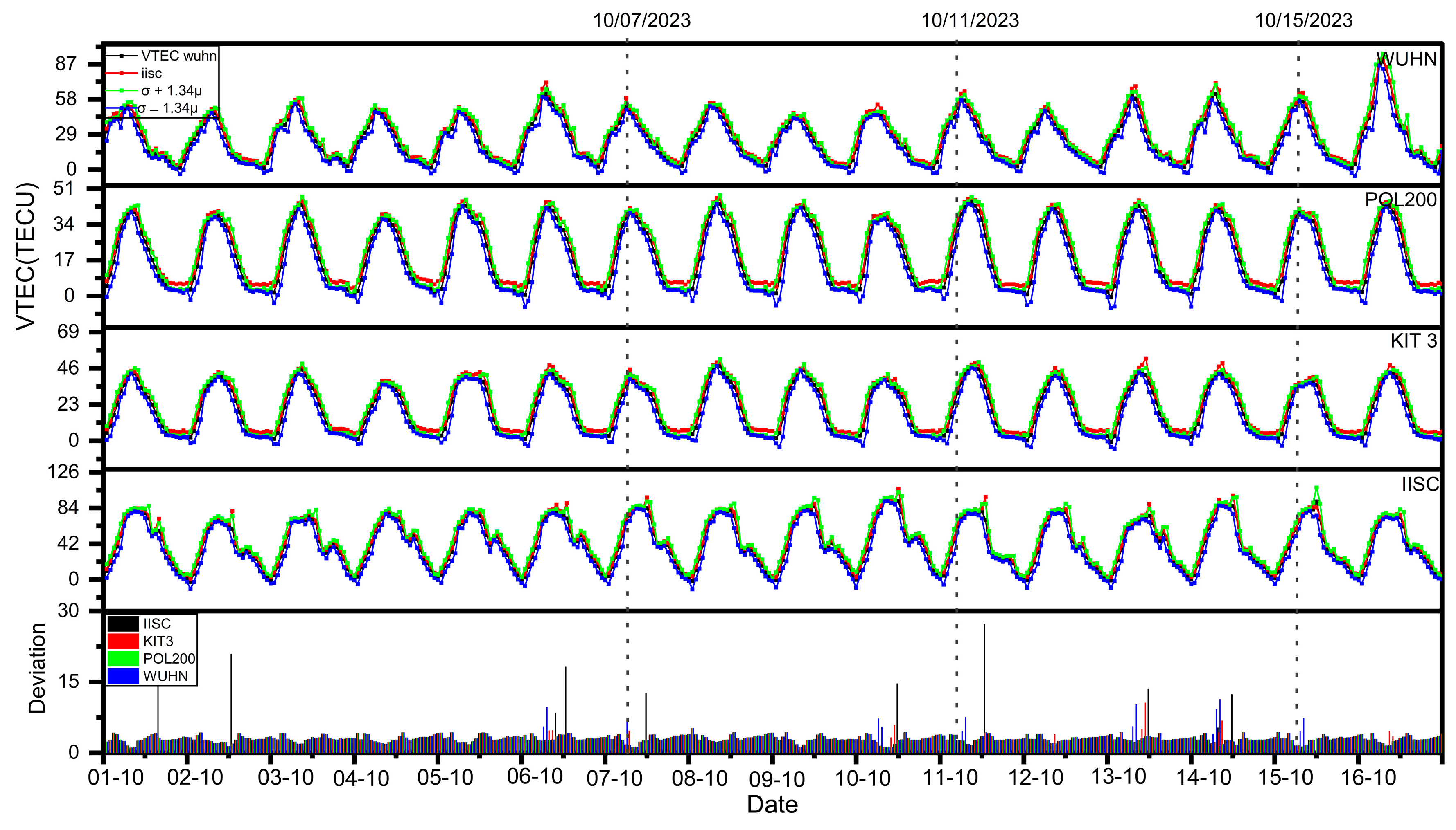
3.1.2. GPS-TEC Anomalies

Based on the anomalous days observed in the GIM data, the GPS stations nearest to the epicenter, such as KIT3, IISC, WUHN, LHAZ, CHUM, and POL200, were selected out of several stations. These finalized stations were considered for anomaly extraction, as shown in Figure 6 and Figure 7. Positive spikes in TEC for the 2015 earthquake can be seen one day before the earthquake on every ground station for almost 30 min, with a prominent difference of 2-8 TECU. On the day following the earthquake, anomalies appeared for POL200 and CHUM, which were the least distant from the epicenter, with a difference of 2-4 TECU, suggesting short-term pre-seismic anomalies.

The 2023 earthquake Swarm event anomalies on 6 October, 1 day before the first earthquake, started appearing around 3-14 UTC. On 7 October, the earthquake happened at 6:40 UTC and the anomalies appeared from 3 to 14 UTC. Following the second earthquake that occurred on 11 October, the prior 3 days’ anomalies were also witnessed. The anomalies on 9 October also appeared from 2 to 13 UTC, those on 10 October appeared from 2:30 to 12:30 UTC, and those on 11 October appeared from 3 to 14 UTC. Also, for 15 October, the anomalies for the third earthquake event appeared at 3-14 UTC on 13 October; those on 14 October appeared at 2-12 UTC; and finally, on the last earthquake day, the anomalies kept on appearing in the same time range as the previous pattern: from 7 to 15 October at 3-12 UTC. The anomalies that appeared were well synchronized with the anomalies appearing in the GIM-TEC and Te and Ne observations; for reference, see Table 1 and

Table 2. Common anomalies prior to the October 2023 earthquake; DOE is day of earthquake.

Date	GIM TEC Anomaly (@UTC)	GPS TEC Anomaly (@UTC)	SWARM Ne and Te Anomaly	Fof2 Anomaly presence	Date	GIM TEC Anomaly (@UTC)	GPS TEC Anomaly (@UTC)	SWARM Ne and Te Anomaly	Fof2 Anomaly presence
21-09-2023	12 (S of epicenter) (+)	-	(−) Te Night	-	07-10-2023 (DOE)	3 (+)	4-6 (+), 12–4 (+)	(−) Te Night	✓
24-09-2023	6, 7 (+)	-	(+) Ne Day	-	10-10-2023	3 (+)	8-13 (+)	(−) Te Day	✓
29-09-2023	8-11 (+)	-	(+) Ne Night\(−) Day/(−) Te Night	-	11-10-2023 (DOE)	10-11 (+)	11-13 (+), 15 (+)	(+) Ne Night\(−) Day/(−) Te Night\Day	✓
30-09-2023	10-13 (+)	-	(+) Ne Night\Day/(−) Te Night	-	13-10-2023	17-23 (+)	12-15 (+), 17-20 (+)	(+) Ne Day/Ne Night/(−) Te Night	✓
01-10-2023	3 (+)	16 (+)	(+) Ne Day/(−) Te Night/(±) Day	-	14-10-2023	1-2((+),21-23((−)	12-14	(−) Te Day/Te Night	✓
02-10-2023	10-13 (+)	14-16 (+)	(+) Ne Night/(−) Te Night/(±) Day	-	15-10-2023 (DOE)	7-9 (+), 21-23 (−)	9-12 (+)	(−) Ne Day/(−) Te Night	✓
06-10-2023	14 (+)	10-12 (+), 14-15 (+)	(+) Ne Day/(±) Te Day	✓	-	-	-	-	-

. To support this statement, it can be seen in Table 1 that the GPS-TEC anomalies appeared almost 11 days before the earthquake day, and the time and durations coincided with the GIM-TEC anomalies; e.g., for the GIM-TEC anomalies, the appearance time was around 9-12 UTC, and the GPS-TEC anomalies appeared from 8 to 12 UTC for the 2015 earthquake cases. Similar coinciding time duration can be seen on the other excluded days and for the 2023 earthquake cases as well.

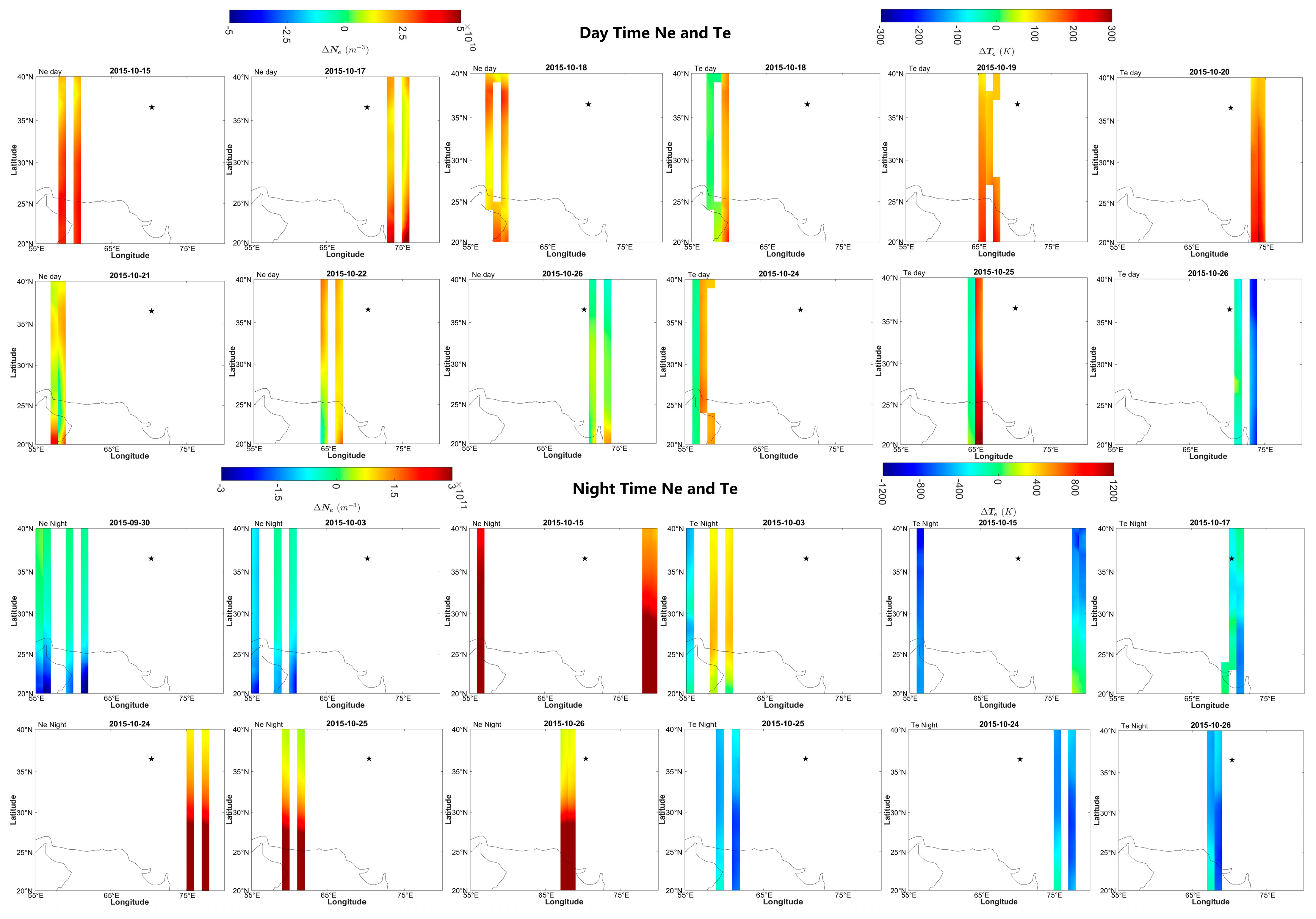
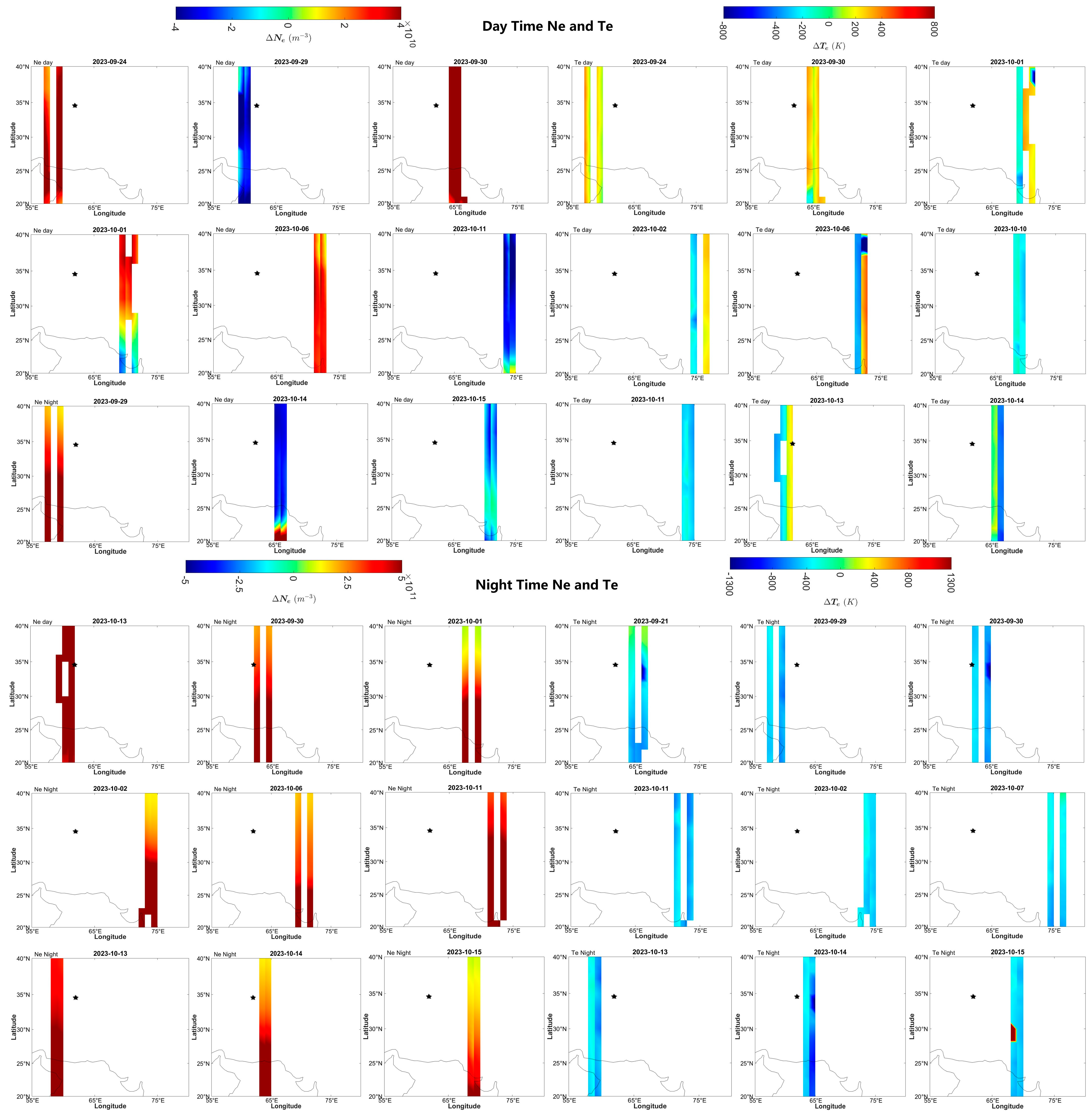
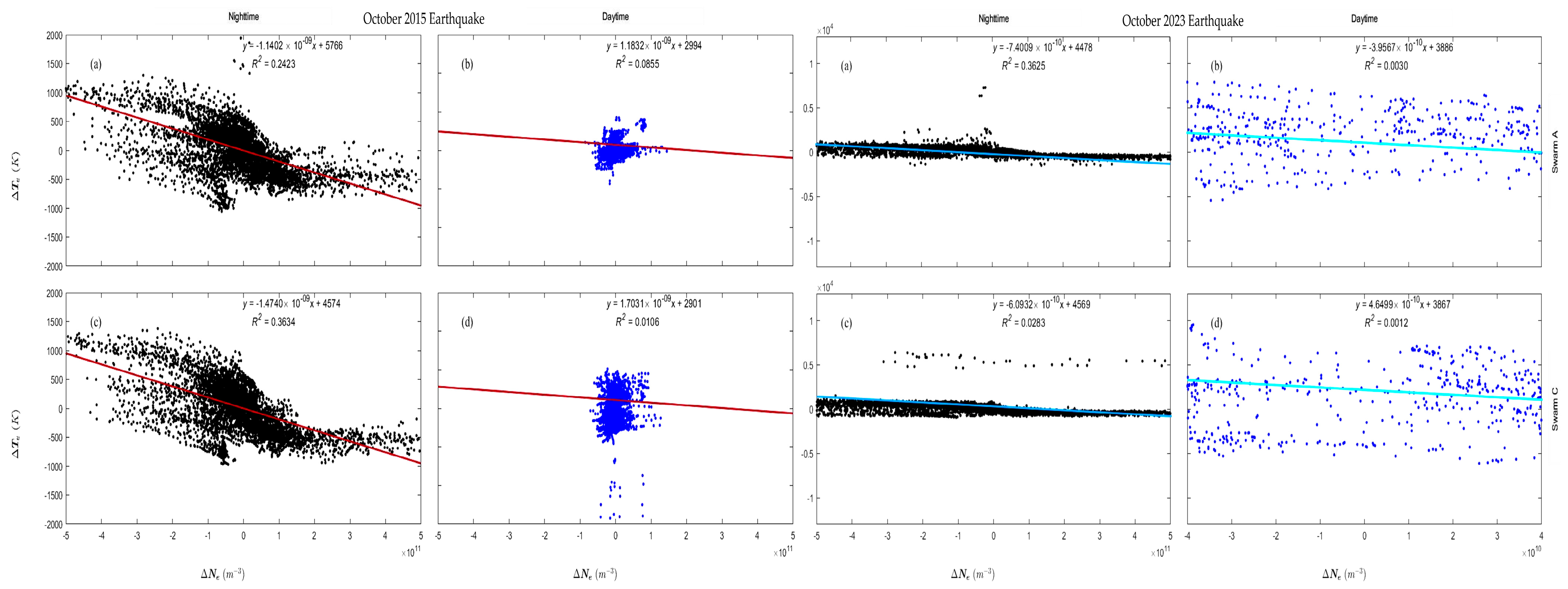
3.1.3. Ne and Te Anomalies

The plasma anomalies were obtained using the revisit trajectory comparison method, which involved processing three months of data from the Swarm A and C satellites. The orbital tracks were divided into two classes based on day and nighttime periods. Background values were removed from these data groups to establish the ΔNe and ΔTe thresholds, which were defined by the 2σ limit. The earthquake occurred on 26 October 2015, and the ΔNe thresholds were 3.11 × 10¹¹ m⁻³ and 5.67 × 10¹⁰ m⁻³ during day and night times, respectively, and the ΔTe thresholds were 1256 K and 809 K. Figure 8 illustrates the results obtained from the Swarm A and C satellites. The disturbances as positive and negative anomalies were witnessed on 18, 19, 21, 22, 23, 24, 28, 29, and 30 September and 17, 18, and 19 of October.

The nighttime Ne anomalies started appearing on September 30(+) and 3 and 7(−) October; there are random positive and negative anomalies on 15,21 October (+). The daytime Ne anomalies can be seen, starting from 30th September (−) and 13(−), 15(+), 17-18(+), 23(+), and on 26 of October (−), the day of the earthquake can be observed.

For the nighttime temperature anomalies, negative anomalies started appearing on 30 September (−). Some short-term positive anomalies occurred from 13 October, while the occurrence of strong negative anomalies can be seen on 15, 17, 24, 25, and 26, these being present in the form of pre- and co-seismic anomalies. Negative Te anomalies continuously occurred from 30 September and 3 October, strong positive anomalies occurred on 19–20 and 24–25 October, and on 26 October, a negative anomaly was observed passing over the earthquake epicenter for the daytime trajectory, as explained in Table 1 and shown in Figure 8 and Figure S3.

The other earthquake happened as a group of earthquakes on 7, 11, and 15 October 2023; the ΔNe thresholds were 4.97 × 10¹¹ m⁻³ and 2.9 × 10¹⁰ m⁻³ during the night and day periods, respectively, and ΔTe thresholds were 1252 K and 739 K.

Excluding solar and geomagnetically disturbed days, Ne anomalies started appearing on September 20 (−) and 29 (+), 30 (+), and 2 (+) of October; the remaining disturbed days were taken as geomagnetically disturbed days, which confirmed the presence of pre-seismic disturbances (Figure 9). Ne daytime anomalies, starting from 20 (+), 22 (−), 24 (+), 27 (+), 28 (−), 29 (−), and 30 (+) September, and 1 (+) and 3 (+) anomalies on 11 and 15 of October (−), on the days of the earthquake, can be observed.

In contrast, in the nighttime Te data, there were negative anomalies that appeared on 21, 22, 23, 29, and 30 September and on 1 and 2 October, while the occurrence of strong negative anomalies from 4 to 15 can be seen, which can be regarded as pre-, co-, and post-seismic anomalies. The daytime Te anomalies continuously occurred from (+)20 and 28(−) September to (±)1, (±)2, and (±)3 October, as explained in Table 2 and shown in Figure 9 and Figure S4.

Figure 10 shows the correlation analysis of ΔNe and ΔTe for Swarm A and Swarm C satellite data during the daytime and overnight periods. The plasma abnormalities show an increasing occurrence on the days preceding the earthquakes. This shows that there is a link between fluctuations in plasma anomalies and seismic activity. The data show a negative association between Ne and Te, which is most prominent during the nighttime observations.

Furthermore, the graphs demonstrate that plasma abnormalities are more noticeable during the day, implying a possible diurnal fluctuation in the association between plasma anomalies and earthquake occurrence.

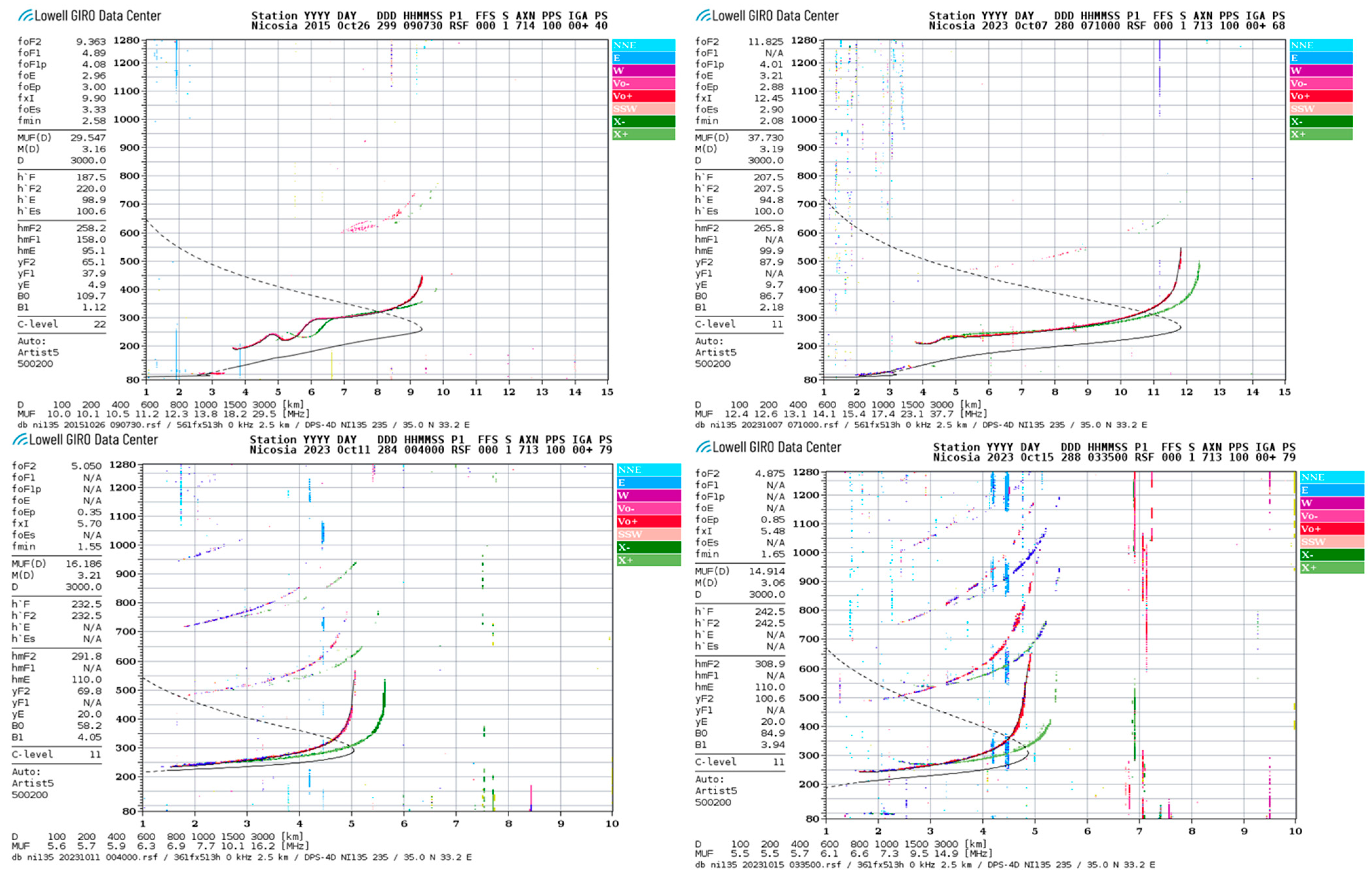
3.1.4. foF2 and hmF2 Anomalies

For the investigation of ionospheric height and density, the ionosonde NI135, located on the island of Cyprus (latitude: 35.03°N, longitude: 33.16°E), was selected based on the availability of data. It is located around 3000 km from the point, which has a comparable latitude (34.5442°N, 61.8891°E). The proximity in latitudes suggests that the ionospheric properties may be similar. Figure 11 shows the ionogram and the related predicted electron concentration profile, which provide visual representations of the data. For the 2015 earthquake, the foF2 shows a wave-like signature of detected disturbance and an increase to 9.363 MHz (from the previously observed frequency of 3.8 MHz on 25 October) almost 2 min before the earthquake, which occurred at 09:09 UTC. For the 2023 earthquakes, the foF2 decreased to 11.825 MHz from the 12.56 MHz observed on 6 October (1 day before the first earthquake), and for later days, the foF2 shows a decreasing trend for the NI135 station, along with the rippled oscillations observed on previous days. For this reason, 2D plots of foF2 and hmF2 were created separately determine the near-to-real values over the earthquake region (Figure S4).

Figure 11 also shows an interesting quasi-periodic pattern inside the foF2 variation. As can be seen, the intensity of each pixel represents the signal strength in the form of electron density profiles, while the colors indicate the wave polarization, angle of arrival, and Doppler frequency. Traces in the ionogram image correspond to individual reflected signals (echoes) observed at each sounding frequency. The ionograms of NI135 for other anomalous days were also analyzed, and coinciding behaviors with TEC and plasma scintillations were found. Intriguingly, the Doppler ionosonde detected a substantial increase in the Doppler frequency three days before the earthquakes, which persisted until the main shock occurred. The ionogram from the NI135 ionospheric station in Cyprus showed a reduction in the key frequency foF2. The 2D critical frequency foF2 plots were also analyzed 10 days before the occurrence of the earthquake in both cases. The unusual changes in foF2 and hmF2 over Afghanistan around 34°N and 62°E are displayed in Figure S5. The critical frequency and height of the ionosphere were verified at the NI135 station and from the ionogram simultaneously, which yielded the following result: for 2015, the 26 October earthquake graph shows a drop in both factors around 8 UTC (from 10.3 MHz to 9.8 MHz in foF2, with the ionospheric height also deviating prominently from the IRI quiet-time climatology, showing a drop in the F2 layer height and density).

The observed abnormal effect in the change in foF2 was unique across the whole observable time frame preceding the Mw 7.5 and Mw 6.3 Afghanistan earthquakes, occurring in a calm geomagnetic state. This shows a possible ionospheric disturbance associated with earthquake preparation, as indicated by the decline in critical frequency fof2, reaching a minimum of 7 days before the 2015 earthquake’s main shock and 9 days before the 2023 earthquake. Also, the anomalies from Table 1 and Table 2 coincide on 17, 18, 19, 20, 24, 25, and 26 October 2015 and on 6, 7, 9, 10, 11, 13, 14, and 15 October 2023, excluding the geomagnetically disturbed days.

4. Discussion

In this study, a spatiotemporal investigation of ionospheric TEC, Ne, Te, foF2, and hmF2 fluctuations preceding the 2015 and 2023 earthquakes in Afghanistan was conducted, indicating significant abnormalities and trends (summarized in Table 1 and Table 2). The TEC values from the GIM and GPS ground stations differed significantly from the expected background levels, indicating the presence of ionospheric disturbances.

The GIM-TEC anomalies observed on 18 October 2015 and 13 October 2023 followed a semi-global pattern. These anomalies coincided with geomagnetic and solar calm days, implying the presence of additional contributing forces, which could possibly be the previous days’ geomagnetic activities, climate variations such as air pressure currents, human activities, radiofrequency interferences, or electromagnetic emissions causing global-scale positive anomalies.

The simultaneous abnormalities detected in ionospheric plasma and critical frequency, both in terms of spatial and temporal aspects, highlight the atypical nature of these specific days, potentially implying a link to seismic activity.

The Ne and Te parameters also showed noticeable variations before the earthquakes, illustrating the ionosphere’s dynamic reaction to seismic activity. The foF2 and ionogram results exhibit fluctuations in the ionospheric height and critical frequency fof2. Furthermore, the lithosphere–atmosphere–ionosphere interaction concept proposes that electric field fluctuations due to radon gas release or gravity waves caused by tectonic stresses might propagate upward and effect the ionosphere. These electric field disturbances can alter plasma density (Ne), electron temperature (Te), and the F2 layer’s critical frequency (foF2). Without exception, ionospheric disturbances have regularly been measured before earthquakes. According to studies, these pre-seismic TEC, Ne, Te, and foF2 anomalies might begin 20–15 days in advance and last until a few minutes before the earthquakes, which also suggests the benefit of LAI coupling [57,58,59]. The fundamental mechanism most likely includes rock stress causing electromagnetic emissions and energy transfer between Earth’s geophysical layers [4]. Multiple data sources confirm a compelling link between ionospheric disturbances and seismic activity, bolstering the notion that these anomalies may foreshadow earthquakes [60]. For instance, Gousheva reinforced this by demonstrating abnormalities in the ionospheric quasi-static electric field during seismic events, implying a possible link between these disturbances and earthquakes [61]. Kouris recognized the potential of ionospheric changes as precursors to seismic occurrences, notwithstanding the need for further research [62]. These investigations reinforce the case for examining the relationship between ionospheric disturbances and seismic activity.

To demonstrate a causal relationship between the detected anomalies and earthquakes, it is critical to examine ionospheric fluctuations caused by upper atmospheric events such as thunderstorms, which are characterized by heavy clouds, intense rainfall, and lightning. Weather conditions during seismic occurrences were tracked using data from EUMETSAT [https://www.eumetsat.int/] and Ventusky. The unusual days and times were compared to local weather conditions, cloud activity, and total rainfall in the earthquake preparation area. This detailed investigation demonstrated that weather conditions were normal throughout the occurrence of anomalies and did not match, providing strong evidence for the presence of real seismic ionospheric disturbances.

5. Conclusions

In this study, we carried out a comprehensive investigation on multi-parameter ionospheric disturbances possibly associated with two major earthquake events in Afghanistan that occurred in 2015 and 2023, with the use of GIM, GPS, Swarm, and ionosonde data; the following phenomena and findings were obtained.

• It was detected that GIM-TEC anomalies for the October 2015 Mw 7.5 earthquake started appearing from 26 days before the shock to 1 day before the shock, while for the 2023 Mw 6.3 earthquake, the Swarm anomalies could be noticed even 2 h before the earthquake happened.
• After stringently examining the common anomaly days, it was found that all possible ionospheric parameters for the 2015 earthquake were 30-09, 03-10, 15-10, 17-10, 18-10, 19-10, 20-10, 24-10, and 25-10, and for the 2023 earthquake, they were 19-09, 21-09, 24-09, 26-09, 29-09, 30-09, 02-10, 06-10, 07-10, 10-10, 11-10, 13-10, 14-10, and 15-10.
• Spatiotemporal coincidence was well established during the multi-parameter analysis, which confirms that the revealed ionospheric anomalies are important precursors of earthquakes.
• The data validations from various sources for anomalous days also confirm the true pre-seismic activities induced in the ionosphere.

To summarize, this approach for ionospheric sounding is a promising method for detecting pre-seismic activity and perhaps increasing earthquake forecasting capabilities. However, it is vital to emphasize that further research on and refining of this technique are still required to properly grasp the complex relationship between ionospheric variability and earthquakes. The study focused only on single-sphere (ionosphere) disturbances prior to earthquakes, but anomalies associated with LAI coupling are also crucial to gain a complete understanding of earthquake preparation and, hence, prediction. The observed anomalies in TEC, Ne, and Te and foF2 point to a potential link between the lithosphere and ionosphere, implying that seismic activity can influence ionospheric properties. The findings lend support to the concept that the ionosphere exhibits precursory behavior before large earthquakes, highlighting its potential as a source for earthquake forecasting. Studying ionospheric disturbances preceding earthquakes holds promise for earthquake monitoring and prediction efforts. However, it is important to note that the relationship between the ionosphere and earthquakes is complex, and not all ionospheric disturbances necessarily indicate an impending earthquake. To efficiently investigate the seismic-derived disturbances, the LCAI model needs to be evaluated, which could be carried out in the future. Further research is needed to deepen our understanding of the underlying mechanisms, as well as establish reliable methodologies for earthquake forecasting and early-warning systems using advanced detection systems.

References

1. Pulinets, S.A. Seismic Activity as a Source of the Ionospheric Variability. Adv. Space Res. 1998, 22, 903–906. [Google Scholar] [CrossRef]
2. Dautermann, T.; Calais, E.; Haase, J.; Garrison, J. Investigation of Ionospheric Electron Content Variations before Earthquakes in Southern California, 2003–2004. J. Geophys. Res. 2007, 112, 2006JB004447. [Google Scholar] [CrossRef]
3. Pulinets, S.A.; Gaivoronska, T.B.; Leyva Contreras, A.; Ciraolo, L. Correlation Analysis Technique Revealing Ionospheric Precursors of Earthquakes. Nat. Hazards Earth Syst. Sci. 2004, 4, 697–702. [Google Scholar] [CrossRef]
4. Qiang, Z.; Xu, X.; Dian, C. Case 27 Thermal Infrared Anomaly Precursor of Impending Earthquakes. PAGEOPH 1997, 149, 159–171. [Google Scholar] [CrossRef]
5. Wu, L.; Liu, S.; Wu, Y. The Experiment Evidences for Tectonic Earthquake Forecasting Based on Anomaly Analysis on Satellite Infrared Image. In Proceedings of the 2006 IEEE International Symposium on Geoscience and Remote Sensing, Denver, CO, USA, 31 July–4 August 2006; pp. 2158–2162. [Google Scholar]
6. Das, N.; Bhandari, R.; Ghose, D.; Sen, P.; Sinha, B. Significant Anomalies of Helium, Radon and Gamma Ahead of 7.9 M China Earthquake. Acta Geod. Geophys. Hung. 2009, 44, 357–365. [Google Scholar] [CrossRef]
7. Wu, L.; Zheng, S.; De Santis, A.; Qin, K.; Di Mauro, R.; Liu, S.; Rainone, M.L. Geosphere Coupling and Hydrothermal Anomalies before the 2009 Mw 6.3 L’Aquila Earthquake in Italy. Nat. Hazards Earth Syst. Sci. 2016, 16, 1859–1880. [Google Scholar] [CrossRef]
8. Pak, Y.E. Linear Electro-Elastic Fracture Mechanics of Piezoelectric Materials. Int. J. Fract. 1992, 54, 79–100. [Google Scholar] [CrossRef]
9. Freund, F.T.; Takeuchi, A.; Lau, B.W.S.; Post, R.; Keefner, J.; Mellon, J.; Al-Manaseer, A. Stress-Induced Changes in the Electrical Conductivity of Igneous Rocks and the Generation of Ground Currents. Terr. Atmos. Ocean. Sci. 2004, 15, 437. [Google Scholar] [CrossRef]
10. Freund, F. Toward a Unified Solid State Theory for Pre-Earthquake Signals. Acta Geophys. 2010, 58, 719–766. [Google Scholar] [CrossRef]
11. Freund, F. Pre-Earthquake Signals: Underlying Physical Processes. J. Asian Earth Sci. 2011, 41, 383–400. [Google Scholar] [CrossRef]
12. Mao, W.; Wu, L.; Liu, S.; Gao, X.; Huang, J.; Xu, Z.; Qi, Y. Additional Microwave Radiation From Experimentally Loaded Granite Covered With Sand Layers: Features and Mechanisms. IEEE Trans. Geosci. Remote Sens. 2020, 58, 5008–5022. [Google Scholar] [CrossRef]
13. Qi, Y.; Wu, L.; Ding, Y.; Mao, W. Microwave Brightness Temperature Anomalies Associated With the 2015 Mw 7.8 Gorkha and Mw 7.3 Dolakha Earthquakes in Nepal. IEEE Trans. Geosci. Remote Sens. 2020, 60, 4500611. [Google Scholar] [CrossRef]
14. Wu, L.; Wang, X.; Qi, Y.; Lu, J.; Mao, W. Characteristics and Mechanisms of Near-Surface Negative Atmospheric Electric Field Anomalies Preceding the 5 September 2022, M s 6.8 Luding Earthquake in China. Nat. Hazards Earth Syst. Sci. 2024, 24, 773–789. [Google Scholar] [CrossRef]
15. Pulinets, S.; Boyarchuk, K. Ionospheric Precursors of Earthquakes; Springer: Berlin, Germany; New York, NY, USA, 2004; ISBN 978-3-540-20839-6. [Google Scholar]
16. Draz, M.U.; Shah, M.; Jamjareegulgarn, P.; Shahzad, R.; Hasan, A.M.; Ghamry, N.A. Deep Machine Learning Based Possible Atmospheric and Ionospheric Precursors of the 2021 Mw 7.1 Japan Earthquake. Remote Sens. 2023, 15, 1904. [Google Scholar] [CrossRef]
17. Gousheva, M.; Glavcheva, R.; Danov, D.; Angelov, P.; Hristov, P.; Kirov, B.; Georgieva, K. Satellite Monitoring of Anomalous Effects in the Ionosphere Probably Related to Strong Earthquakes. Adv. Space Res. 2006, 37, 660–665. [Google Scholar] [CrossRef]
18. He, L.; Heki, K. Ionospheric Anomalies Immediately before Mw7.0–8.0 Earthquakes. J. Geophys. Res. 2017, 122, 8659–8678. [Google Scholar] [CrossRef]
19. Li, W.; Yue, J.; Guo, J.; Yang, Y.; Zou, B.; Shen, Y.; Zhang, K. Statistical Seismo-Ionospheric Precursors of M7.0+ Earthquakes in Circum-Pacific Seismic Belt by GPS TEC Measurements. Adv. Space Res. 2018, 61, 1206–1219. [Google Scholar] [CrossRef]
20. Xie, T.; Chen, B.; Wu, L.; Dai, W.; Kuang, C.; Miao, Z. Detecting Seismo-Ionospheric Anomalies Possibly Associated With the 2019 Ridgecrest (California) Earthquakes by GNSS, CSES, and Swarm Observations. JGR Space Phys. 2021, 126, e2020JA028761. [Google Scholar] [CrossRef]
21. Ruwali, A.; Kumar, A.J.S.; Prakash, K.B.; Sivavaraprasad, G.; Ratnam, D.V. Implementation of Hybrid Deep Learning Model (LSTM-CNN) for Ionospheric TEC Forecasting Using GPS Data. IEEE Geosci. Remote Sens. Lett. 2021, 18, 1004–1008. [Google Scholar] [CrossRef]
22. Li, Q.; Yang, D.; Fang, H. Two Hours Ahead Prediction of the TEC over China Using a Deep Learning Method. Universe 2022, 8, 405. [Google Scholar] [CrossRef]
23. Xie, T.; Dai, Z.; Zhu, X.; Chen, B.; Ran, C. LSTM-Based Short-Term Ionospheric TEC Forecast Model and Positioning Accuracy Analysis. GPS Solut. 2023, 27, 66. [Google Scholar] [CrossRef]
24. Jeong, S.; Lee, W.K.; Kil, H.; Jang, S.; Kim, J.; Kwak, Y. Deep Learning-Based Regional Ionospheric Total Electron Content Prediction—Long Short-Term Memory (LSTM) and Convolutional LSTM Approach. Space Weather 2024, 22, e2023SW003763. [Google Scholar] [CrossRef]
25. He, L.M.; Wu, L.X.; De Santis, A.; Liu, S.J.; Yang, Y. Is There a One-to-One Correspondence between Ionospheric Anomalies and Large Earthquakes along Longmenshan Faults? Ann. Geophys. 2014, 32, 187–196. [Google Scholar] [CrossRef]
26. He, L.; Wu, L.; Liu, S.; Ma, B. Seismo-Ionospheric Anomalies Detection Based on Integrated Wavelet. In Proceedings of the 2011 IEEE International Geoscience and Remote Sensing Symposium, Vancouver, BC, Canada, 24–29 July 2011; pp. 1834–1837. [Google Scholar]
27. Pulinets, S.; Krankowski, A.; Hernandez-Pajares, M.; Marra, S.; Cherniak, I.; Zakharenkova, I.; Rothkaehl, H.; Kotulak, K.; Davidenko, D.; Blaszkiewicz, L.; et al. Ionosphere Sounding for Pre-Seismic Anomalies Identification (INSPIRE): Results of the Project and Perspectives for the Short-Term Earthquake Forecast. Front. Earth Sci. 2021, 9, 610193. [Google Scholar] [CrossRef]
28. Iwata, T.; Umeno, K. Pre-Seismic Ionospheric Anomalies Detected before the 2016 Kumamoto Earthquake. JGR Space Phys. 2017, 122, 3602–3616. [Google Scholar] [CrossRef]
29. Kandalyan, R.A.; Alquran, M.K. Ionosphere Scintillation and Earthquakes. Jordan J. Phys. 2010, 3, 69–76. [Google Scholar]
30. Xu, T.; Wu, J.; Zhao, Z.; Liu, Y.; He, S.; Li, J.; Wu, Z.; Hu, Y. Brief Communication “Monitoring Ionospheric Variations before Earthquakes Using the Vertical and Oblique Sounding Network over China”. Nat. Hazards Earth Syst. Sci. 2011, 11, 1083–1089. [Google Scholar] [CrossRef]
31. Parrot, M.; Benoist, D.; Berthelier, J.J.; Błęcki, J.; Chapuis, Y.; Colin, F.; Elie, F.; Fergeau, P.; Lagoutte, D.; Lefeuvre, F.; et al. The Magnetic Field Experiment IMSC and Its Data Processing Onboard DEMETER: Scientific Objectives, Description and First Results. Planet. Space Sci. 2006, 54, 441–455. [Google Scholar] [CrossRef]
32. Marchetti, D.; Akhoondzadeh, M. Analysis of Swarm Satellites Data Showing Seismo-Ionospheric Anomalies around the Time of the Strong Mexico (Mw = 8.2) Earthquake of 08 September 2017. Adv. Space Res. 2018, 62, 614–623. [Google Scholar] [CrossRef]
33. Liu, J.Y.; Chen, Y.I.; Chuo, Y.J.; Chen, C.S. A Statistical Investigation of Preearthquake Ionospheric Anomaly. J. Geophys. Res. 2006, 111, 2005JA011333. [Google Scholar] [CrossRef]
34. Cherrier, N.; Castaings, T.; Boulch, A. Deep Sequence-to-Sequence Neural Networks for Ionospheric Activity Map Prediction. In Neural Information Processing; Liu, D., Xie, S., Li, Y., Zhao, D., El-Alfy, E.-S.M., Eds.; Lecture Notes in Computer Science; Springer International Publishing: Cham, Switzerland, 2017; Volume 10638, pp. 545–555. ISBN 978-3-319-70138-7. [Google Scholar]
35. Salikhov, N.; Shepetov, A.; Pak, G.; Nurakynov, S.; Kaldybayev, A.; Ryabov, V.; Zhukov, V. Investigation of the Pre- and Co-Seismic Ionospheric Effects from the 6 February 2023 M7.8 Turkey Earthquake by a Doppler Ionosonde. Atmosphere 2023, 14, 1483. [Google Scholar] [CrossRef]
36. Sharma, G.; Nayak, K.; Romero-Andrade, R.; Aslam, M.A.M.; Sarma, K.K.; Aggarwal, S.P. Low Ionosphere Density Above the Earthquake Epicentre Region of Mw 7.2, El Mayor–Cucapah Earthquake Evident from Dense CORS Data. J. Indian Soc. Remote Sens. 2024, 52, 543–555. [Google Scholar] [CrossRef]
37. Tachema, A. Identifying Pre-Seismic Ionospheric Disturbances Using Space Geodesy: A Case Study of the 2011 Lorca Earthquake (Mw 5.1), Spain. Earth Sci. Inform. 2024, 1–17. [Google Scholar] [CrossRef]
38. Nayak, K.; Romero-Andrade, R.; Sharma, G.; Zavala, J.L.C.; Urias, C.L.; Trejo Soto, M.E.; Aggarwal, S.P. A Combined Approach Using B-Value and Ionospheric GPS-TEC for Large Earthquake Precursor Detection: A Case Study for the Colima Earthquake of 7.7 Mw, Mexico. Acta Geod. Geophys. 2023, 58, 515–538. [Google Scholar] [CrossRef]
39. Song, J.; Kang, S.-H.; Han, D.-H.; Kim, B.-G.; Kee, C. Real-Time Detection of Seismic Ionospheric Disturbance Using Global Navigation Satellite System Signal. JKSAS 2019, 47, 549–557. [Google Scholar] [CrossRef]
40. Marchand, R.; Berthelier, J.J. Simple Model for Post Seismic Ionospheric Disturbances above an Earthquake Epicentre and along Connecting Magnetic Field Lines. Nat. Hazards Earth Syst. Sci. 2008, 8, 1341–1347. [Google Scholar] [CrossRef]
41. Sezen, U.; Arikan, F.; Arikan, O.; Ugurlu, O.; Sadeghimorad, A. Online, Automatic, Near-real Time Estimation of GPS-TEC: IONOLAB-TEC. Space Weather 2013, 11, 297–305. [Google Scholar] [CrossRef]
42. Yasyukevich, Y.V.; Kiselev, A.V.; Zhivetiev, I.V.; Edemskiy, I.K.; Syrovatskii, S.V.; Maletckii, B.M.; Vesnin, A.M. SIMuRG: System for Ionosphere Monitoring and Research from GNSS. GPS Solut. 2020, 24, 69. [Google Scholar] [CrossRef]
43. Hayes, G.P.; Meyers, E.K.; Dewey, J.W.; Briggs, R.W.; Earle, P.S.; Benz, H.M.; Smoczyk, G.M.; Flamme, H.E.; Barnhart, W.D.; Gold, R.D.; et al. Tectonic Summaries of Magnitude 7 and Greater Earthquakes from 2000 to 2015. US Geol. Surv. 2017, 148. [Google Scholar] [CrossRef]
44. Ghassabian, N.N. Afghanistan Earthquake Swarm 10-29-2023; Brill: Leiden, The Netherlands, 2023. [Google Scholar] [CrossRef]
45. Wu, L.; Qin, K.; Liu, S. GEOSS-Based Thermal Parameters Analysis for Earthquake Anomaly Recognition. Proc. IEEE 2012, 100, 2891–2907. [Google Scholar] [CrossRef]
46. Qin, K.; Wu, L.; Zheng, S.; Liu, S. A Deviation-Time-Space-Thermal (DTS-T) Method for Global Earth Observation System of Systems (GEOSS)-Based Earthquake Anomaly Recognition: Criterions and Quantify Indices. Remote Sens. 2013, 5, 5143–5151. [Google Scholar] [CrossRef]
47. Dobrovolsky, I.P.; Zubkov, S.I.; Miachkin, V.I. Estimation of the Size of Earthquake Preparation Zones. PAGEOPH 1979, 117, 1025–1044. [Google Scholar] [CrossRef]
48. Oikonomou, C. Investigation of Ionospheric TEC Precursors Related to the M7.8 Nepal and M8.3 Chile Earthquakes in 2015 Based on Spectral and Statistical Analysis. Nat. Hazards 2016, 83, 97–116. [Google Scholar] [CrossRef]
49. Nayak, K.; López-Urías, C.; Romero-Andrade, R.; Sharma, G.; Guzmán-Acevedo, G.M.; Trejo-Soto, M.E. Ionospheric Total Electron Content (TEC) Anomalies as Earthquake Precursors: Unveiling the Geophysical Connection Leading to the 2023 Moroccan 6.8 Mw Earthquake. Geosciences 2023, 13, 319. [Google Scholar] [CrossRef]
50. Colonna, R.; Filizzola, C.; Genzano, N.; Lisi, M.; Tramutoli, V. Optimal Setting of Earthquake-Related Ionospheric TEC (Total Electron Content) Anomalies Detection Methods: Long-Term Validation over the Italian Region. Geosciences 2023, 13, 150. [Google Scholar] [CrossRef]
51. Van Den IJssel, J.; Encarnação, J.; Doornbos, E.; Visser, P. Precise Science Orbits for the Swarm Satellite Constellation. Adv. Space Res. 2015, 56, 1042–1055. [Google Scholar] [CrossRef]
52. De Santis, A.; Balasis, G.; Pavón-Carrasco, F.J.; Cianchini, G.; Mandea, M. Potential Earthquake Precursory Pattern from Space: The 2015 Nepal Event as Seen by Magnetic Swarm Satellites. Earth Planet. Sci. Lett. 2017, 461, 119–126. [Google Scholar] [CrossRef]
53. Liu, J.; Huang, J.; Zhang, X. Ionospheric Perturbations in Plasma Parameters before Global Strong Earthquakes. Adv. Space Res. 2014, 53, 776–787. [Google Scholar] [CrossRef]
54. Ondoh, T. Investigation of Precursory Phenomena in the Ionosphere, Atmosphere and Groundwater before Large Earthquakes of M>6.5. Adv. Space Res. 2009, 43, 214–223. [Google Scholar] [CrossRef]
55. Pulinets, S.A.; Legen’ka, A.D.; Gaivoronskaya, T.V.; Depuev, V.K. Main Phenomenological Features of Ionospheric Precursors of Strong Earthquakes. J. Atmos. Sol. Terr. Phys. 2003, 65, 1337–1347. [Google Scholar] [CrossRef]
56. Global Ionosphere Radio Observatory. 2023. Available online: https://giro.uml.edu/ (accessed on 1 November 2023).
57. Wu, L.; Qi, Y.; Mao, W.; Lu, J.; Ding, Y.; Peng, B.; Xie, B. Scrutinizing and Rooting the Multiple Anomalies of Nepal Earthquake Sequence in 2015 with the Deviation–Time–Space Criterion and Homologous Lithosphere–Coversphere–Atmosphere–Ionosphere Coupling Physics. Nat. Hazards Earth Syst. Sci. 2023, 23, 231–249. [Google Scholar] [CrossRef]
58. Kamogawa, M. Preseismic Lithosphere-atmosphere-ionosphere Coupling. Eos Trans. 2006, 87, 417–424. [Google Scholar] [CrossRef]
59. Khan, A.Q.; Ghaffar, B.; Shah, M.; Ullah, I.; Oliveira-Júnior, J.F.; Eldin, S.M. Possible Seismo-Ionospheric Anomalies Associated with the 2016 Mw 6.5 Indonesia Earthquake from GPS TEC and Swarm Satellites. Front. Astron. Space Sci. 2022, 9, 1065453. [Google Scholar] [CrossRef]
60. Haider, S.F.; Shah, M.; Li, B.; Jamjareegulgarn, P.; De Oliveira-Júnior, J.F.; Zhou, C. Synchronized and Co-Located Ionospheric and Atmospheric Anomalies Associated with the 2023 Mw 7.8 Turkey Earthquake. Remote Sens. 2024, 16, 222. [Google Scholar] [CrossRef]
61. Gousheva, M.; Danov, D.; Hristov, P.; Matova, M. Quasi-Static Electric Fields Phenomena in the Ionosphere Associated with Pre- and Post Earthquake Effects. Nat. Hazards Earth Syst. Sci. 2008, 8, 101–107. [Google Scholar] [CrossRef]
62. Kouris, S.S.; Spalla, P.; Zolesi, B. Could Ionospheric Variations Be Precursors of a Seismic Event? A Short Discussion. Ann. Geophys. 2001, 44, 23. [Google Scholar] [CrossRef]
Figure 1. Tectonic settings of Afghanistan earthquake cases along with ionosondes and GNSS ground stations.
Remotesensing 16 01839 g001
Figure 2. The technical route of excluding, processing, and verifying the ionospheric anomalies prior to seismic activities.
Remotesensing 16 01839 g002
Figure 3. Solar–geomagnetic weather conditions (a) prior to 26 October 2015 earthquake, where 20 and 21 September and 4–10 and 14 October were excluded due to active solar and geomagnetic events, and (b) prior to 7–15 October 2023 earthquake, where 2, 13, 19, and 26 September were excluded. The dark blue curved lines and blue shaded bars represents the daily variation of Dst index, Kp*10 (10 multiplied by Kp) and F10.7 indices respectively, while the dashed vertical line represents the day of earthquakes.
Remotesensing 16 01839 g003
Figure 4. GIM anomalies prior to 26 October 2015 earthquake; magnetic equator (red line), earthquake epicenter (green circle enclosed black star), positive anomalies over epicenter (red cloud), and negative anomalies (blue cloud) are shown.
Remotesensing 16 01839 g004
Figure 5. The GIM anomalies prior to October 2023 earthquakes are shown, with the magnetic equator (red line), earthquake epicenter (green circle enclosed black star), positive anomalies over the epicenter (red cloud), and negative anomalies (blue cloud).
Remotesensing 16 01839 g005
Figure 6. For the 2015 earthquake days between 12 and 27 October, the CHUM, IISC, LHAZ, and POL200 ground stations were selected, where the mean VTEC (black line), LSTM-derived VTEC (red line), upper envelope (green line) and lower envelope (blue line), and earthquake day (dotted gray line) are shown.
Remotesensing 16 01839 g006
Figure 7. For the 2023 earthquake days between 1 and 16 October, the WUHN, POL200, KIT3, and IISC ground stations were selected, where the mean VTEC (black line), LSTM-derived VTEC (red line), upper envelope (red line) and lower envelope (green line), and earthquake day (dotted gray line) are shown.
Remotesensing 16 01839 g007
Figure 8. Ionospheric plasma Ne and Te anomalies prior to the 26 October 2015 earthquake for the nightside orbit (descending around 23:00) and the dayside orbit (ascending around 11:00). Black star represents the earthquake epicenter and gray line shows the costal boundaries.
Remotesensing 16 01839 g008
Figure 9. Ionospheric Ne and Te anomalies prior to the 7, 11, and 15 October 2023 earthquakes for the nightside orbit (descending around 23:00) and the diurnal orbit (ascending around 11:00). Black star represents the earthquake epicenter and gray line shows the costal boundaries.
Remotesensing 16 01839 g009
Figure 10. The mutual correlation of the day and nighttime ∆Ne and ∆Te anomalies of the Swarm A and C satellites, for 2015 and 2023 earthquake cases respectively, the red and cyan lines are the regression lines.
Remotesensing 16 01839 g010
Figure 11. NI135 ionogram from the DID based on the 26 October 2015 and 7, 11, and 15 October 2023 reflectivity, illustrating frequency versus trip time around 2–4 min before each earthquake, where the Y-axis is height (km) and x-axis is frequency (MHz). Red: O-polarization echoes (vertical); green: X-polarization echoes. Real-time EDP using O-traces (thin black lines) and computed bottom-side EDP (black line with uncertainty bars) [56].
Remotesensing 16 01839 g011