
GeoSparseNet: A Multi-Source Geometry-Aware CNN for Urban Scene Analysis

 , , , , , ,
  and
and 
Abstract
1. Introduction
Motivation
- Quality of Classification: Urban environments pose challenges for semantic classification due to the complex interplay between man-made and natural elements. While typical algorithms excel in categorizing large continuous surfaces, they struggle with precise object delineation, especially in areas with subtle visual differences. Our method addresses this by employing a geometry-aware approach that effectively distinguishes between planar and non-planar surfaces using the Large Kernel Attention (LKA) edge collapse technique, thereby enhancing classification accuracy in such challenging spaces.
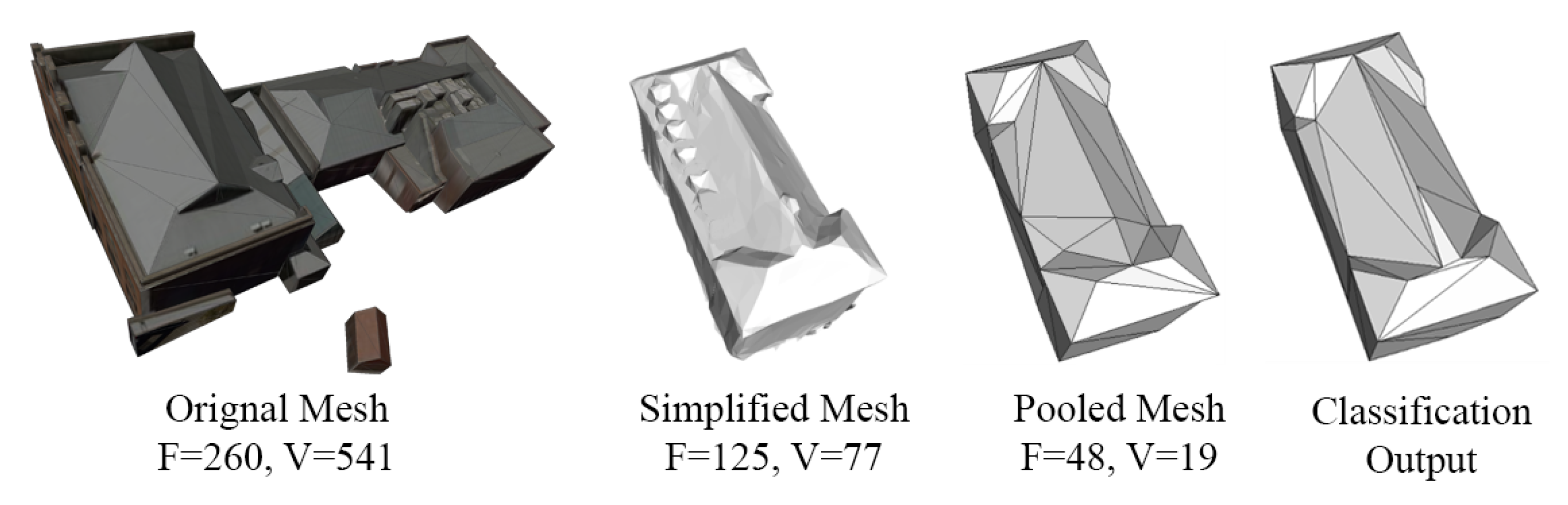
- Distinctive Geometric Features: Semantically classifying 3D data involves assigning single labels to individual points or objects in 3D space, focusing on labeling elements rather than coherent scene segmentation. However, utilizing attributes at the local component level, like groups of triangles (nodes, edges), limits the derived features to a confined area, lacking broader contextual relationships. Distinctive feature abstraction is crucial for effective classification predictions in mesh-based geometric learning. Our approach achieves both local and global geometric feature acquisition by employing LKA-based edge collapse, removing redundant edges while preserving vital ones through task-oriented pooling and unpooling operations.
- Efficiency: Current deep learning techniques encounter challenges in handling large-scale 3D data, especially concerning extensive urban environments. This limitation has been identified previously by Landrieu et al. [10] and further acknowledged in subsequent work like Hui et al. [11]. Following the principles established in prior research focused on improving efficiency, our method introduces distinctive local and non-local characteristics tailored for enhanced classification, leveraging Afzal et al. [12]’s Scaled Cosine Similarity Loss (SCSL). GeoSparseNet aims to advance semantic classification and improve object delineation within large-scale urban meshes.
2. Related Work
2.1. Semantic Classification of Urban Models
2.2. Attention Mechanism
3. Materials and Methods
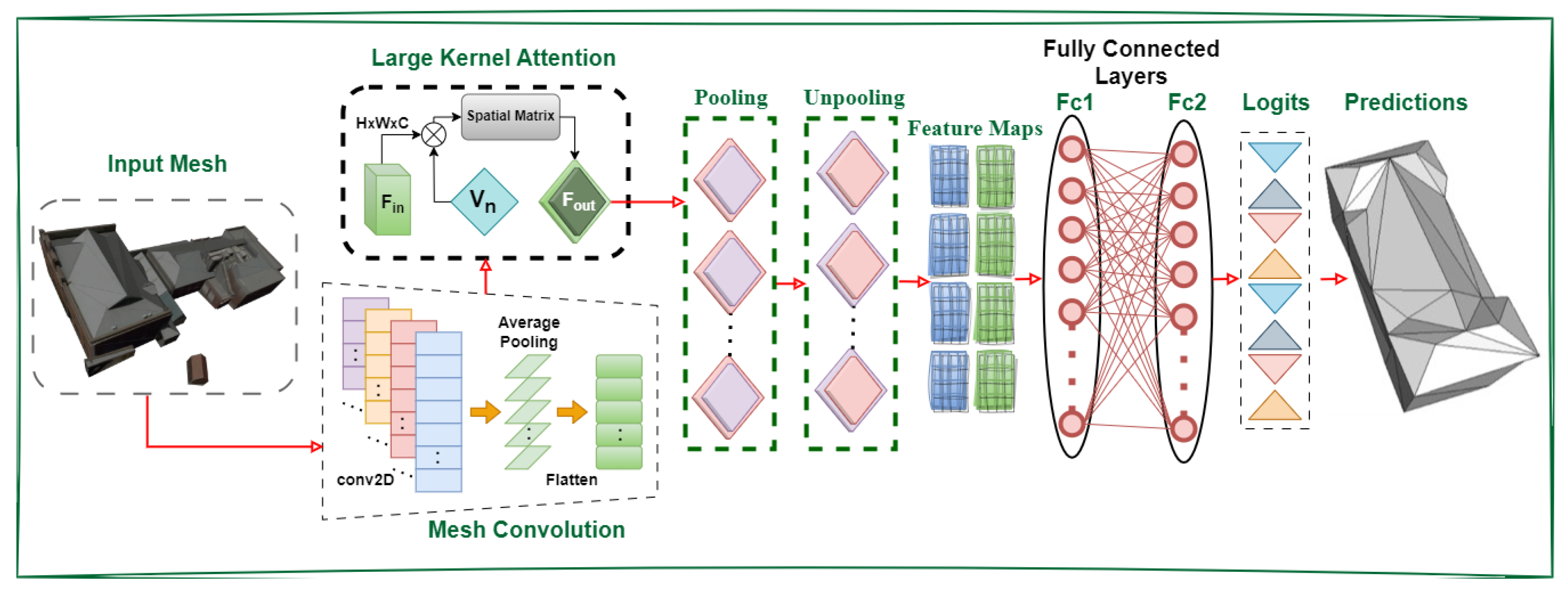
3.1. GeoSparseNet Architecture
3.1.1. Convolution
3.1.2. Large Kernel Attention (LKA)
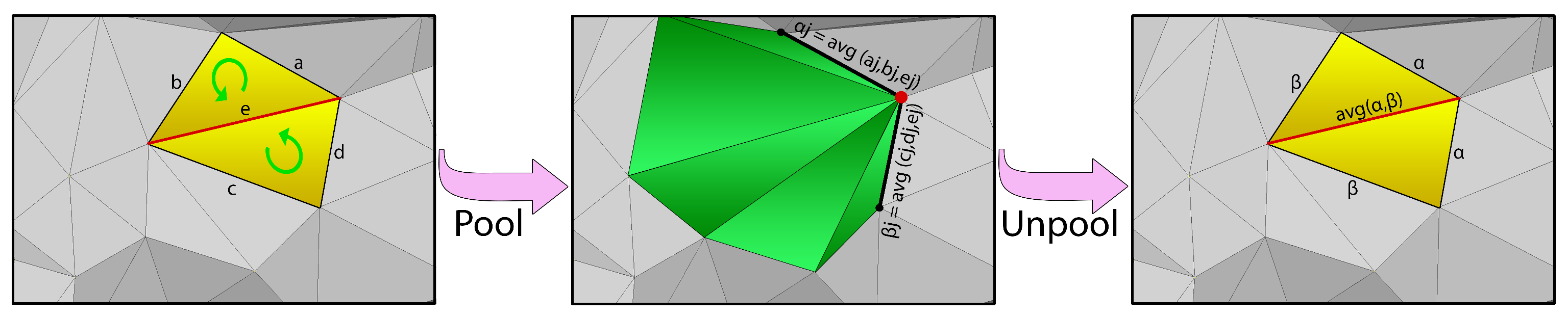
3.1.3. Pooling
3.1.4. Unpooling
3.1.5. Loss Function
4. Results
4.1. Network Configurations
- System settings:
- The experiments were conducted using NVIDIA GeForce RTX 2080Ti GPUs on an Ubuntu operating system.
- Network settings:
- Kernel size , Adam optimizer with learning rate , , , and .
- Parameters settings:
- Pooling resolution , number of convolution filters , and iterations .
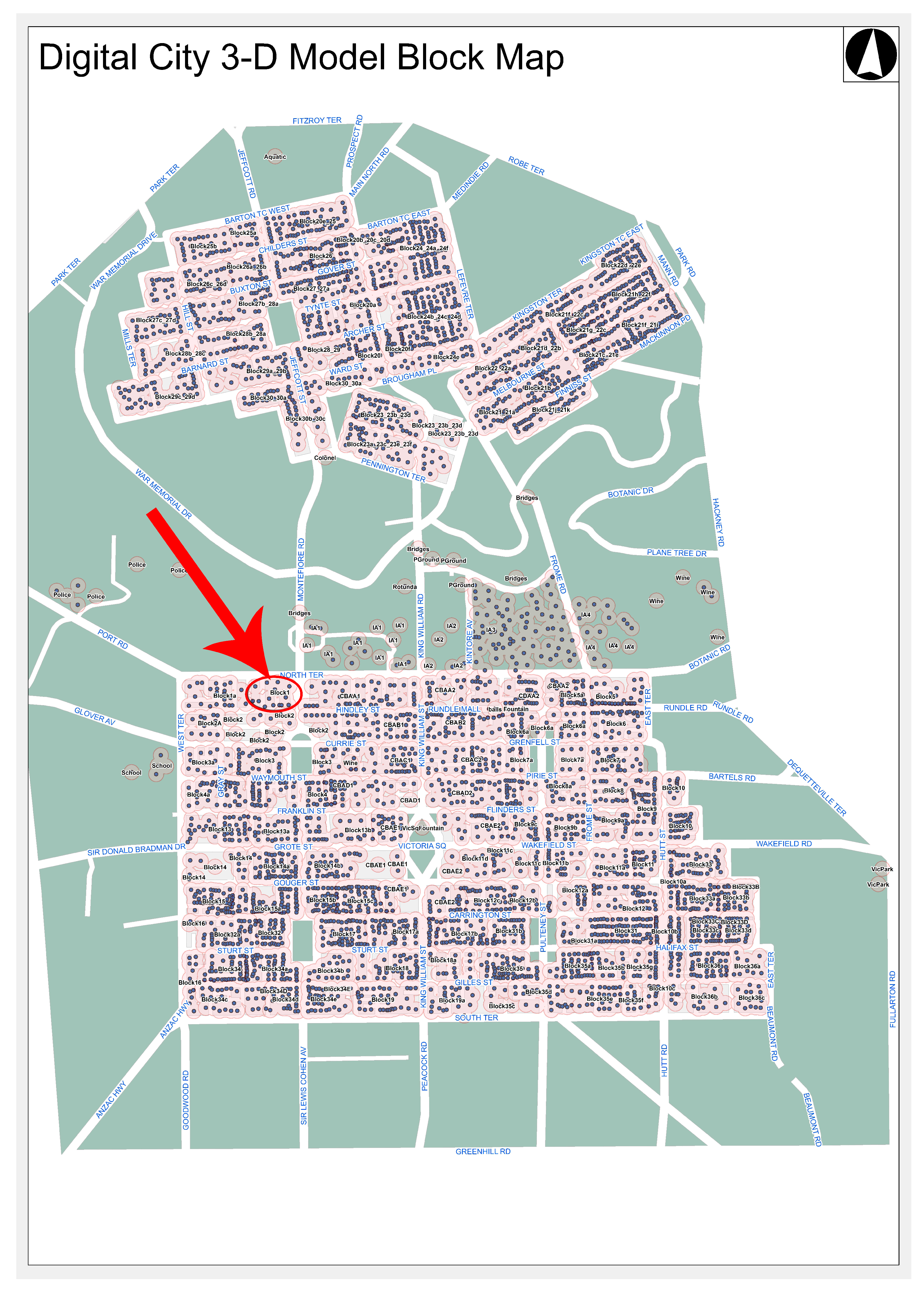
4.2. Adelaide Dataset
- City Blocks:
- Origin(X) 278,434.0000, Origin(Y) 6,130,514.0000, Altitude(AHD) 125.0000
- Balls:
- Origin(X) 281,063.3990, Origin(Y) 6,132,895.2440, Altitude(AHD) 44.9000
- Rotunda:
- Origin(X) 278,434.0000, Origin(Y) 6,130,514.0000, Altitude(AHD) 125.0000
- Vic_Pk_Fountain:
- Origin(X) 280,771.9397, Origin(Y) 6,132,324.6420, Altitude(AHD) 45.0633
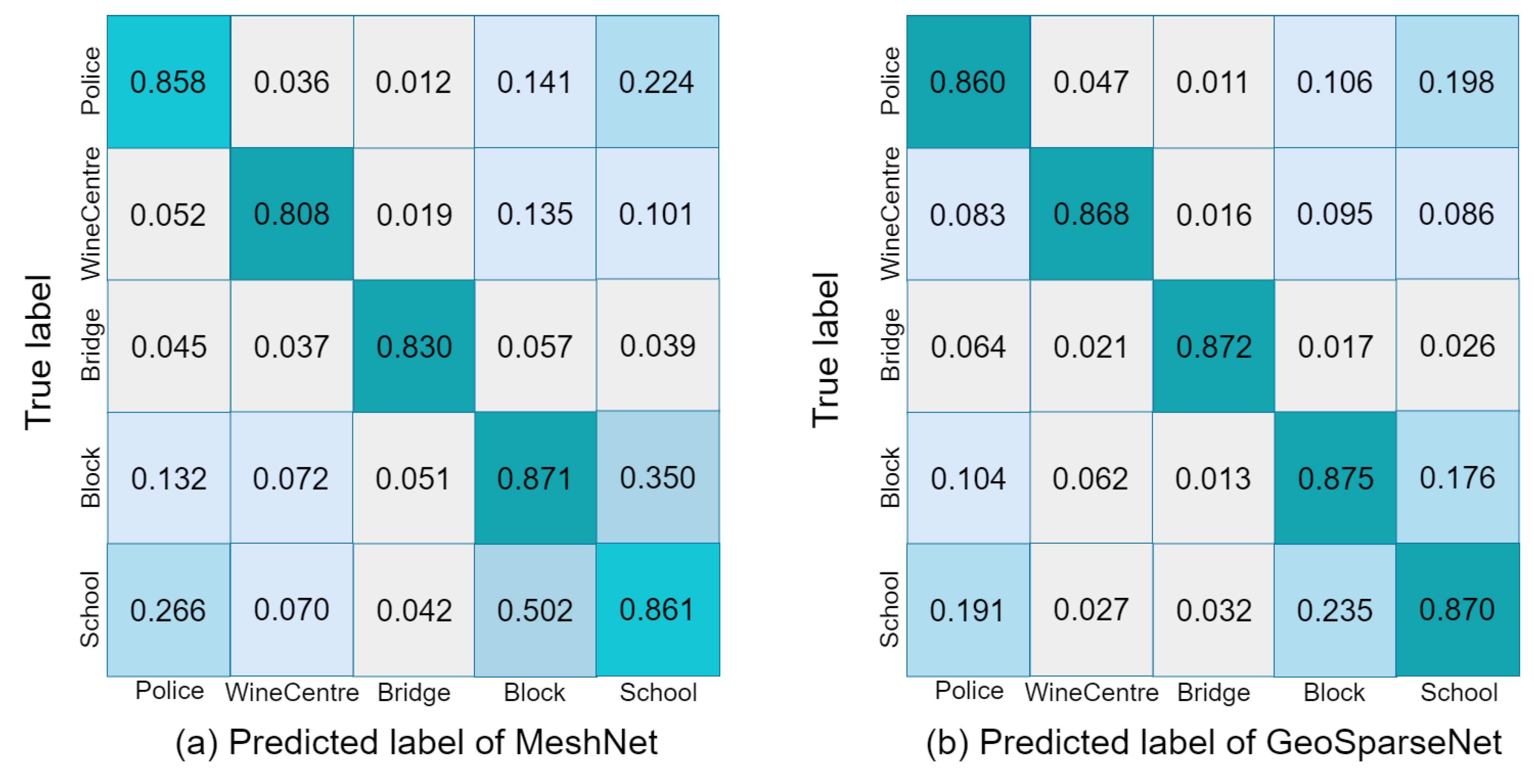
4.3. Evaluation of GeoSparseNet
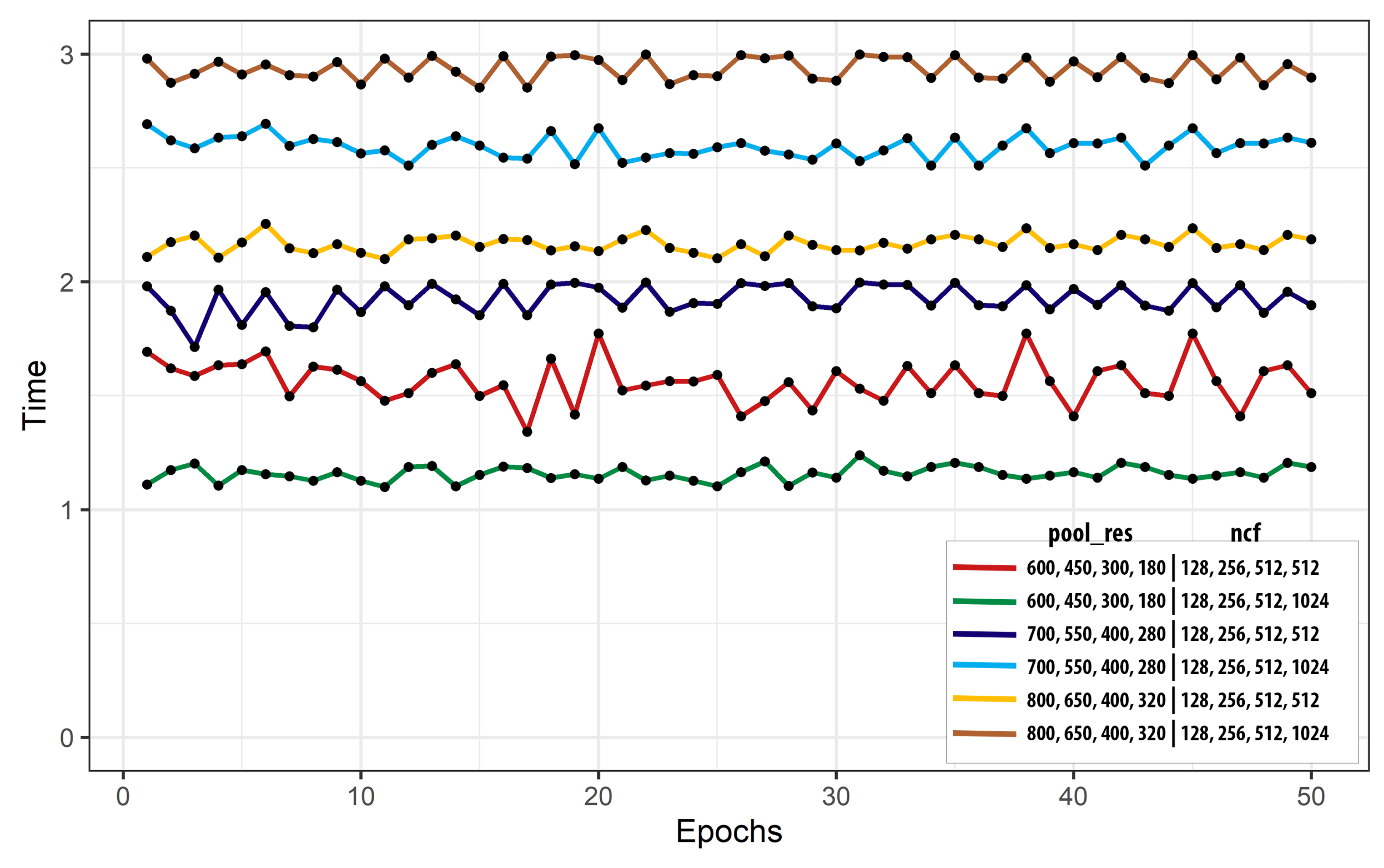
4.4. Computational Complexity
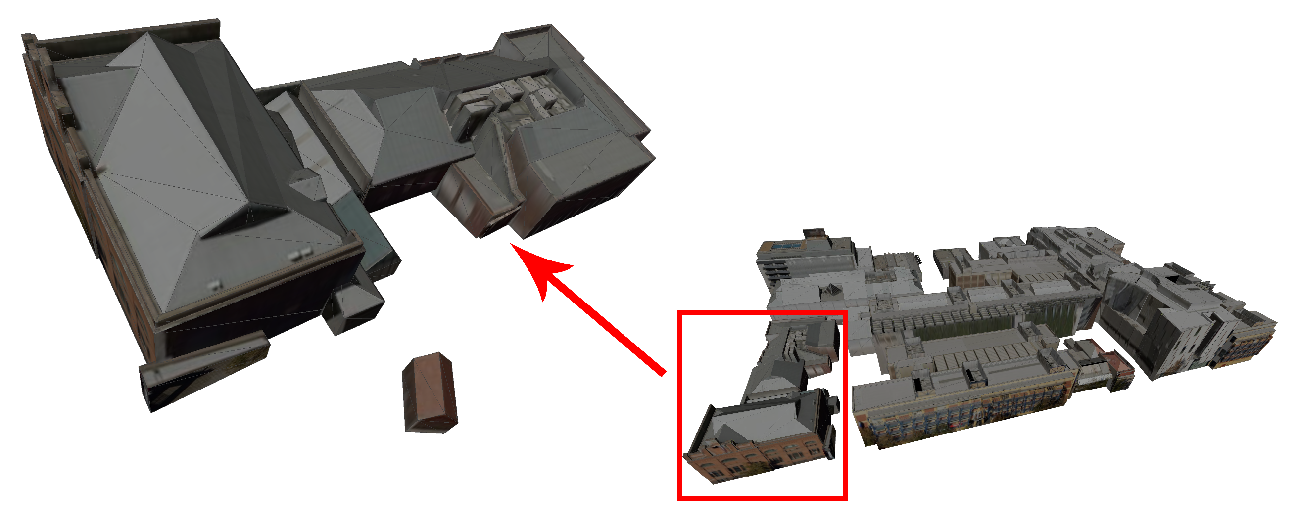
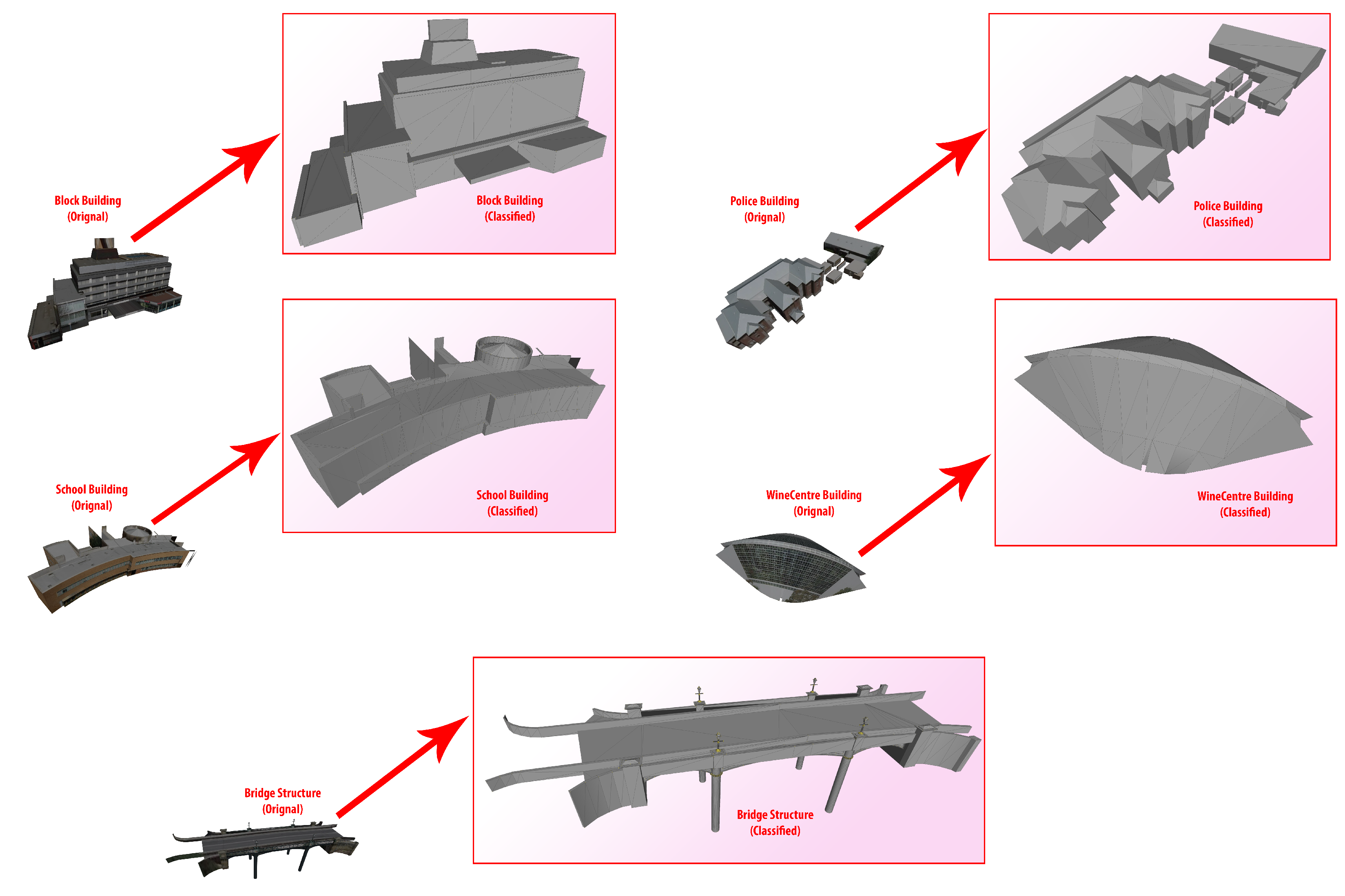
4.5. Results Visualization
5. Discussion
6. Conclusions
Author Contributions
Funding
Data Availability Statement
Conflicts of Interest
References
- Gao, W.; Nan, L.; Boom, B.; Ledoux, H. SUM: A benchmark dataset of semantic urban meshes. ISPRS J. Photogramm. Remote Sens. 2021, 179, 108–120. [Google Scholar] [CrossRef]
- Besuievsky, G.; Beckers, B.; Patow, G. Skyline-based geometric simplification for urban solar analysis. Graph. Model. 2018, 95, 42–50. [Google Scholar] [CrossRef]
- Adam, J.M.; Liu, W.; Zang, Y.; Afzal, M.K.; Bello, S.A.; Muhammad, A.U.; Wang, C.; Li, J. Deep learning-based semantic segmentation of urban-scale 3D meshes in remote sensing: A survey. Int. J. Appl. Earth Obs. Geoinf. 2023, 121, 103365. [Google Scholar] [CrossRef]
- Hackel, T.; Wegner, J.D.; Schindler, K. Fast semantic segmentation of 3D point clouds with strongly varying density. ISPRS J. Photogramm. Remote Sens. 2016, 3, 177–184. [Google Scholar] [CrossRef]
- Thomas, H.; Qi, C.R.; Deschaud, J.E.; Marcotegui, B.; Goulette, F.; Guibas, L.J. Kpconv: Flexible and deformable convolution for point clouds. In Proceedings of the IEEE/CVF, Seoul, Republic of Korea, 27 October–2 November 2019; IEEE: Piscataway, NJ, USA, 2019; pp. 6411–6420. [Google Scholar]
- Selvaraju, P.; Nabail, M.; Loizou, M.; Maslioukova, M.; Averkiou, M.; Andreou, A.; Chaudhuri, S.; Kalogerakis, E. BuildingNet: Learning to label 3D buildings. In Proceedings of the IEEE/CVF, Nashville, TN, USA, 20–25 June 2021; IEEE: Piscataway, NJ, USA, 2021; pp. 10397–10407. [Google Scholar]
- Fu, H.; Jia, R.; Gao, L.; Gong, M.; Zhao, B.; Maybank, S.; Tao, D. 3D-future: 3D furniture shape with texture. Int. J. Comput. Vis. 2021, 129, 3313–3337. [Google Scholar] [CrossRef]
- Mao, Z.; Huang, X.; Xiang, H.; Gong, Y.; Zhang, F.; Tang, J. Glass façade segmentation and repair for aerial photogrammetric 3D building models with multiple constraints. Int. J. Appl. Earth Obs. Geoinf. 2023, 118, 103242. [Google Scholar] [CrossRef]
- Wang, S.; Liu, X.; Zhang, Y.; Li, J.; Zou, S.; Wu, J.; Tao, C.; Liu, Q.; Cai, G. Semantic-guided 3D building reconstruction from triangle meshes. Int. J. Appl. Earth Obs. Geoinf. 2023, 119, 103324. [Google Scholar] [CrossRef]
- Landrieu, L.; Boussaha, M. Point cloud oversegmentation with graph-structured deep metric learning. In Proceedings of the IEEE/CVF, Seoul, Republic of Korea, 27 October–2 November 2019; IEEE: Piscataway, NJ, USA, 2019; pp. 7440–7449. [Google Scholar]
- Hui, L.; Yuan, J.; Cheng, M.; Xie, J.; Zhang, X.; Yang, J. Superpoint network for point cloud oversegmentation. In Proceedings of the IEEE/CVF, Nashville, TN, USA, 20–25 June 2021; IEEE: Piscataway, NJ, USA, 2021; pp. 5510–5519. [Google Scholar]
- Afzal, M.K.; Adam, J.M.; Afzal, H.R.; Zang, Y.; Bello, S.A.; Wang, C.; Li, J. Discriminative feature abstraction by deep L2 hypersphere embedding for 3D mesh CNNs. Inf. Sci. 2022, 607, 1158–1173. [Google Scholar] [CrossRef]
- Ulku, I.; Akagündüz, E. A survey on deep learning-based architectures for semantic segmentation on 2d images. Appl. Artif. Intell. 2022, 36, 2032924. [Google Scholar] [CrossRef]
- Rook, M. Automatic Thematic and Semantic Classification of 3D City Models. Master’s Thesis, TU Delft, Delft, The Netherlands, 2016. [Google Scholar]
- Guo, Y.; Wang, H.; Hu, Q.; Liu, H.; Liu, L.; Bennamoun, M. Deep learning for 3d point clouds: A survey. IEEE Trans. Pattern Anal. Mach. Intell. 2020, 43, 4338–4364. [Google Scholar] [CrossRef]
- Luo, Y.; Wang, H.; Lv, X. End-to-End Edge-Guided Multi-Scale Matching Network for Optical Satellite Stereo Image Pairs. Remote Sens. 2024, 16, 882. [Google Scholar] [CrossRef]
- Shen, S.; Xia, Y.; Eich, A.; Xu, Y.; Yang, B.; Stilla, U. SegTrans: Semantic Segmentation With Transfer Learning for MLS Point Clouds. IEEE Geosci. Remote Sens. Lett. 2023, 20, 6501105. [Google Scholar] [CrossRef]
- Xia, Y.; Wu, Q.; Li, W.; Chan, A.B.; Stilla, U. A lightweight and detector-free 3d single object tracker on point clouds. IEEE Trans. Intell. Transp. Syst. 2023, 24, 5543–5554. [Google Scholar] [CrossRef]
- Li, X.; Liu, Y.; Xia, Y.; Lakshminarasimhan, V.; Cao, H.; Zhang, F.; Stilla, U.; Knoll, A. Fast and deterministic (3 + 1) DOF point set registration with gravity prior. ISPRS J. Photogramm. Remote Sens. 2023, 199, 118–132. [Google Scholar] [CrossRef]
- Huang, J.; Zhou, Y.; Niessner, M.; Shewchuk, J.R.; Guibas, L.J. Quadriflow: A scalable and robust method for quadrangulation. In Computer Graphics Forum; Wiley Online Library: Hoboken, NJ, USA, 2018; Volume 37, pp. 147–160. [Google Scholar]
- Huang, J.; Zhang, H.; Yi, L.; Funkhouser, T.; Nießner, M.; Guibas, L.J. Texturenet: Consistent local parametrizations for learning from high-resolution signals on meshes. In Proceedings of the IEEE/CVF, Seoul, Republic of Korea, 27 October–2 November 2019; IEEE: Piscataway, NJ, USA, 2019; pp. 4440–4449. [Google Scholar]
- Yang, Y.; Liu, S.; Pan, H.; Liu, Y.; Tong, X. PFCNN: Convolutional neural networks on 3D surfaces using parallel frames. In Proceedings of the IEEE/CVF, Seoul, Republic of Korea, 27 October–2 November 2019; IEEE: Piscataway, NJ, USA, 2020; pp. 13578–13587. [Google Scholar]
- Li, Y.; Wu, J.; Liu, H.; Ren, J.; Xu, Z.; Zhang, J.; Wang, Z. Classification of Typical Static Objects in Road Scenes Based on LO-Net. Remote Sens. 2024, 16, 663. [Google Scholar] [CrossRef]
- Wilk, Ł.; Mielczarek, D.; Ostrowski, W.; Dominik, W.; Krawczyk, J. Semantic urban mesh segmentation based on aerial oblique images and point clouds using deep learning. Int. Arch. Photogramm. Remote Sens. Spat. Inf. Sci. 2022, 43, 485–491. [Google Scholar] [CrossRef]
- Zhang, R.; Zhang, G.; Yin, J.; Jia, X.; Mian, A. Mesh-based DGCNN: Semantic Segmentation of Textured 3D Urban Scenes. IEEE Trans. Geosci. Remote Sens. 2023, 61, 4402812. [Google Scholar] [CrossRef]
- Geng, J.; Yu, K.; Sun, M.; Xie, Z.; Huang, R.; Wang, Y.; Zhao, Q.; Liu, J. Construction and Optimisation of Ecological Networks in High-Density Central Urban Areas: The Case of Fuzhou City, China. Remote Sens. 2023, 15, 5666. [Google Scholar] [CrossRef]
- Peng, B.; Yang, J.; Li, Y.; Zhang, S. Land-Use Optimization Based on Ecological Security Pattern—A Case Study of Baicheng, Northeast China. Remote Sens. 2023, 15, 5671. [Google Scholar] [CrossRef]
- Mnih, V.; Heess, N.; Graves, A.; Kavukcuoglu, K. Recurrent models of visual attention. In Proceedings of the NeurIPS, Montreal, QC, Canada, 8–13 December 2014; Curran Associates, Inc.: New York, NY, USA, 2014; Volume 27. [Google Scholar]
- Hu, J.; Shen, L.; Sun, G. Squeeze-and-excitation networks. In Proceedings of the IEEE/CVF, Salt Lake City, UT, USA, 18–23 June 2018; IEEE: Piscataway, NJ, USA, 2018; pp. 7132–7141. [Google Scholar]
- Woo, S.; Park, J.; Lee, J.Y.; Kweon, I.S. Cbam: Convolutional block attention module. In Proceedings of the ECCV, Munich, Germany, 8–14 September 2018; Springer: Berlin/Heidelberg, Germany, 2018; pp. 3–19. [Google Scholar]
- Dai, J.; Qi, H.; Xiong, Y.; Li, Y.; Zhang, G.; Hu, H.; Wei, Y. Deformable Convolutional Networks. In Proceedings of the ICCV, Venice, Italy, 22–29 October 2017; IEEE: Piscataway, NJ, USA, 2017; pp. 764–773. [Google Scholar]
- Hu, H.; Gu, J.; Zhang, Z.; Dai, J.; Wei, Y. Relation networks for object detection. In Proceedings of the IEEE/CVF, Salt Lake City, UT, USA, 18–23 June 2018; IEEE: Piscataway, NJ, USA, 2018; pp. 3588–3597. [Google Scholar]
- Yuan, Y.; Chen, X.; Wang, J. Object-contextual representations for semantic segmentation. In Proceedings of the ECCV, Glasgow, UK, 23–28 August 2020; Springer: Berlin/Heidelberg, Germany, 2020; pp. 173–190. [Google Scholar]
- Geng, Z.; Guo, M.H.; Chen, H.; Li, X.; Wei, K.; Lin, Z. Is attention better than matrix decomposition? arXiv 2021, arXiv:2109.04553. [Google Scholar]
- Guo, M.H.; Xu, T.X.; Liu, J.J.; Liu, Z.N.; Jiang, P.T.; Mu, T.J.; Zhang, S.H.; Martin, R.R.; Cheng, M.M.; Hu, S.M. Attention mechanisms in computer vision: A survey. Comput. Vis. Media 2022, 8, 331–368. [Google Scholar] [CrossRef]
- Vaswani, A.; Shazeer, N.; Parmar, N.; Uszkoreit, J.; Jones, L.; Gomez, A.N.; Kaiser, Ł.; Polosukhin, I. Attention is all you need. In Proceedings of the NeurIPS, Long Beach, CA, USA, 4–9 December 2017; Curran Associates, Inc.: New York, NY, USA, 2017; Volume 30. [Google Scholar]
- Devlin, J.; Chang, M.W.; Lee, K.; Toutanova, K. Bert: Pre-training of deep bidirectional transformers for language understanding. arXiv 2018, arXiv:1810.04805. [Google Scholar]
- Wang, X.; Girshick, R.; Gupta, A.; He, K. Non-local neural networks. In Proceedings of the IEEE/CVF, Salt Lake City, UT, USA, 18–23 June 2018; IEEE: Piscataway, NJ, USA, 2018; pp. 7794–7803. [Google Scholar]
- Fu, J.; Liu, J.; Tian, H.; Li, Y.; Bao, Y.; Fang, Z.; Lu, H. Dual attention network for scene segmentation. In Proceedings of the IEEE/CVF, Seoul, Republic of Korea, 27 October–2 November 2019; IEEE: Piscataway, NJ, USA, 2019; pp. 3146–3154. [Google Scholar]
- Zhang, H.; Goodfellow, I.; Metaxas, D.; Odena, A. Self-attention generative adversarial networks. In Proceedings of the ICML, Long Beach, CA, USA, 9–15 June 2019; PMLR: Cambridge, MA, USA, 2019; pp. 7354–7363. [Google Scholar]
- Dosovitskiy, A.; Beyer, L.; Kolesnikov, A.; Weissenborn, D.; Zhai, X.; Unterthiner, T.; Dehghani, M.; Minderer, M.; Heigold, G.; Gelly, S.; et al. An image is worth 16x16 words: Transformers for image recognition at scale. arXiv 2020, arXiv:2010.11929. [Google Scholar]
- Liu, Z.; Lin, Y.; Cao, Y.; Hu, H.; Wei, Y.; Zhang, Z.; Lin, S.; Guo, B. Swin transformer: Hierarchical vision transformer using shifted windows. In Proceedings of the IEEE/CVF, Nashville, TN, USA, 20–25 June 2021; IEEE: Piscataway, NJ, USA, 2021; pp. 10012–10022. [Google Scholar]
- Wang, W.; Xie, E.; Li, X.; Fan, D.P.; Song, K.; Liang, D.; Lu, T.; Luo, P.; Shao, L. Pyramid vision transformer: A versatile backbone for dense prediction without convolutions. In Proceedings of the IEEE/CVF, Nashville, TN, USA, 20–25 June 2021; IEEE: Piscataway, NJ, USA, 2021; pp. 568–578. [Google Scholar]
- Basu, S.; Gallego-Posada, J.; Viganò, F.; Rowbottom, J.; Cohen, T. Equivariant mesh attention networks. arXiv 2022, arXiv:2205.10662. [Google Scholar]
- Han, X.; Gao, H.; Pfaff, T.; Wang, J.X.; Liu, L.P. Predicting physics in mesh-reduced space with temporal attention. arXiv 2022, arXiv:2201.09113. [Google Scholar]
- Milano, F.; Loquercio, A.; Rosinol, A.; Scaramuzza, D.; Carlone, L. Primal-dual mesh convolutional neural networks. Adv. Neural Inf. Process. Syst. 2020, 33, 952–963. [Google Scholar]
- Yuan, Y.; Huang, L.; Guo, J.; Zhang, C.; Chen, X.; Wang, J. OCNet: Object Context Network for Scene Parsing. arXiv 2018, arXiv:1809.00916. [Google Scholar]
- Guo, M.H.; Lu, C.Z.; Liu, Z.N.; Cheng, M.M.; Hu, S.M. Visual attention network. Comput. Vis. Media 2023, 9, 733–752. [Google Scholar] [CrossRef]
- Berg, M.; Cheong, O.; Kreveld, M.; Overmars, M. Computational Geometry: Algorithms and Applications; Springer: Berlin/Heidelberg, Germany, 2008. [Google Scholar]
- Australia, L.G. [Dataset] Aerial Largescale 3D Mesh Model Dataset of the City of Adelaide Australia. 2022. Available online: https://data.sa.gov.au/data/dataset/3d-model (accessed on 6 March 2024).
- Qi, C.R.; Su, H.; Mo, K.; Guibas, L.J. Pointnet: Deep learning on point sets for 3d classification and segmentation. In Proceedings of the IEEE Conference on Computer Vision and Pattern Recognition, Honolulu, HI, USA, 21–26 July 2017; pp. 652–660. [Google Scholar]
- Qi, C.R.; Yi, L.; Su, H.; Guibas, L.J. Pointnet++: Deep hierarchical feature learning on point sets in a metric space. In Proceedings of the Advances in Neural Information Processing Systems, Long Beach, CA, USA, 4–9 December 2017; Volume 30. [Google Scholar]
- Liu, W.; Lai, B.; Wang, C.; Cai, G.; Su, Y.; Bian, X.; Li, Y.; Chen, S.; Li, J. Ground camera image and large-scale 3-D image-based point cloud registration based on learning domain invariant feature descriptors. IEEE J. Sel. Top. Appl. Earth Obs. Remote Sens. 2020, 14, 997–1009. [Google Scholar] [CrossRef]
- Li, Y.; Bu, R.; Sun, M.; Wu, W.; Di, X.; Chen, B. Pointcnn: Convolution on x-transformed points. In Proceedings of the Advances in Neural Information Processing Systems, Montreal, QC, Canada, 3–8 December 2018; Volume 31. [Google Scholar]
- Li, Y.; Xu, L.; Rao, J.; Guo, L.; Yan, Z.; Jin, S. A Y-Net deep learning method for road segmentation using high-resolution visible remote sensing images. Remote Sens. Lett. 2019, 10, 381–390. [Google Scholar] [CrossRef]
- Feng, Y.; Feng, Y.; You, H.; Zhao, X.; Gao, Y. Meshnet: Mesh neural network for 3d shape representation. In Proceedings of the AAAI Conference on Artificial Intelligence, Honolulu, HI, USA, 27 January–1 February 2019; Volume 33, pp. 8279–8286. [Google Scholar]
- Gröger, G.; Kolbe, T.H.; Nagel, C.; Häfele, K.H. OGC City Geography Markup Language (CityGML) Encoding Standard; Open Geospatial Consortium: Arlington, VA, USA, 2012; p. 344. [Google Scholar]

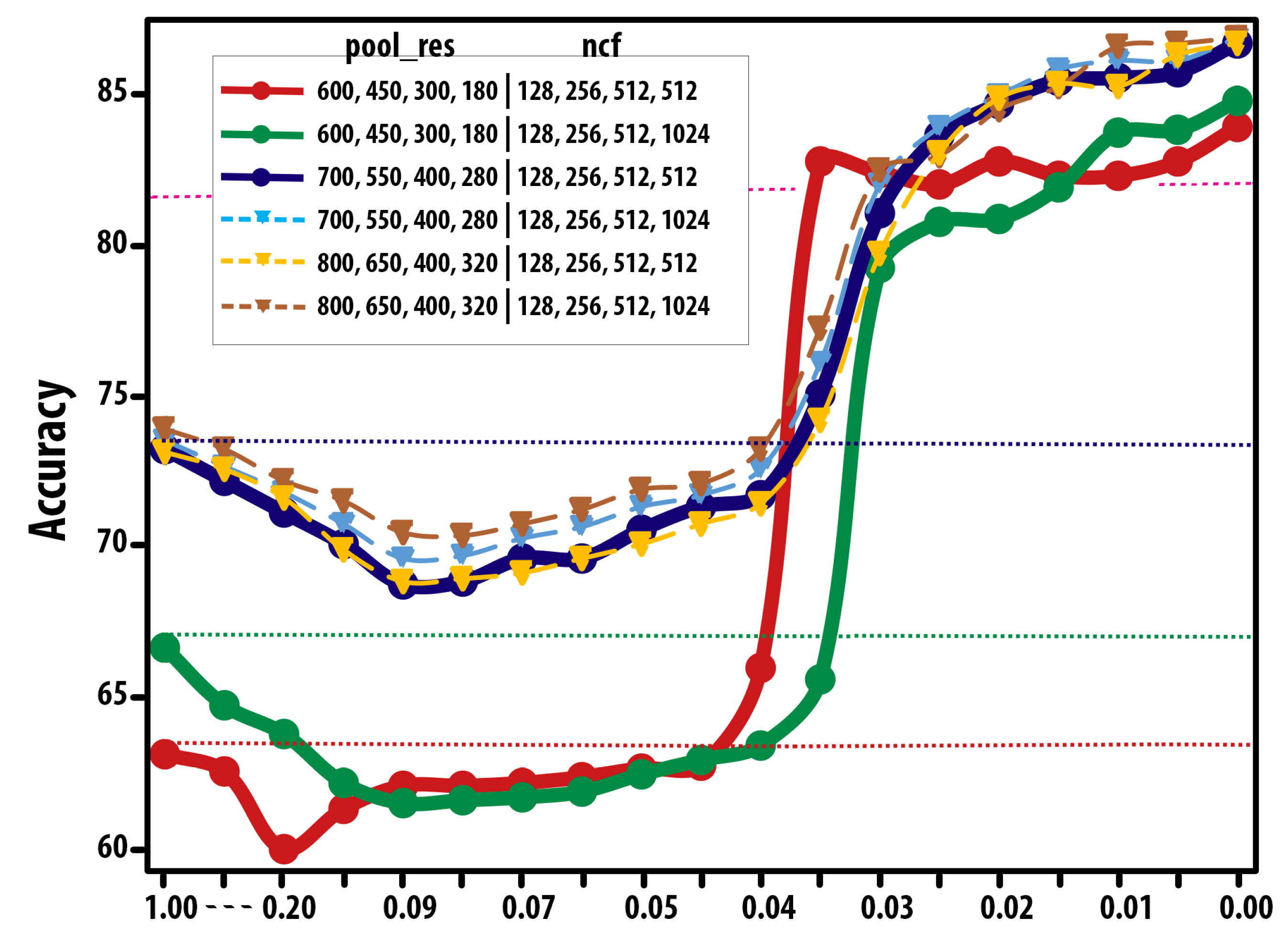
| pool_res | ncf | Accuracy (%) |
|---|---|---|
| 600, 450, 300, 180 | 128, 256, 512, 512 | 83.7 |
| 600, 450, 300, 180 | 128, 256, 512, 1024 | 84.5 |
| 700, 550, 400, 280 | 128, 256, 512, 512 | 86.1 |
| 700, 550, 400, 280 | 128, 256, 512, 1024 | 87.2 |
| 800, 650, 400, 320 | 128, 256, 512, 512 | 86.7 |
| 800, 650, 400, 320 | 128, 256, 512, 1024 | 87.5 |
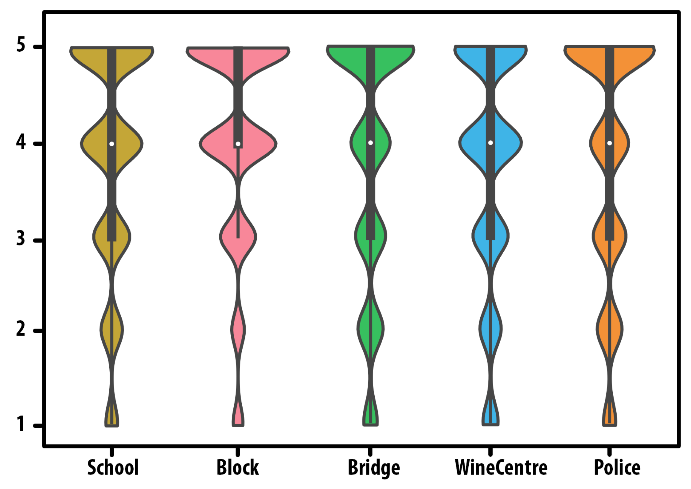
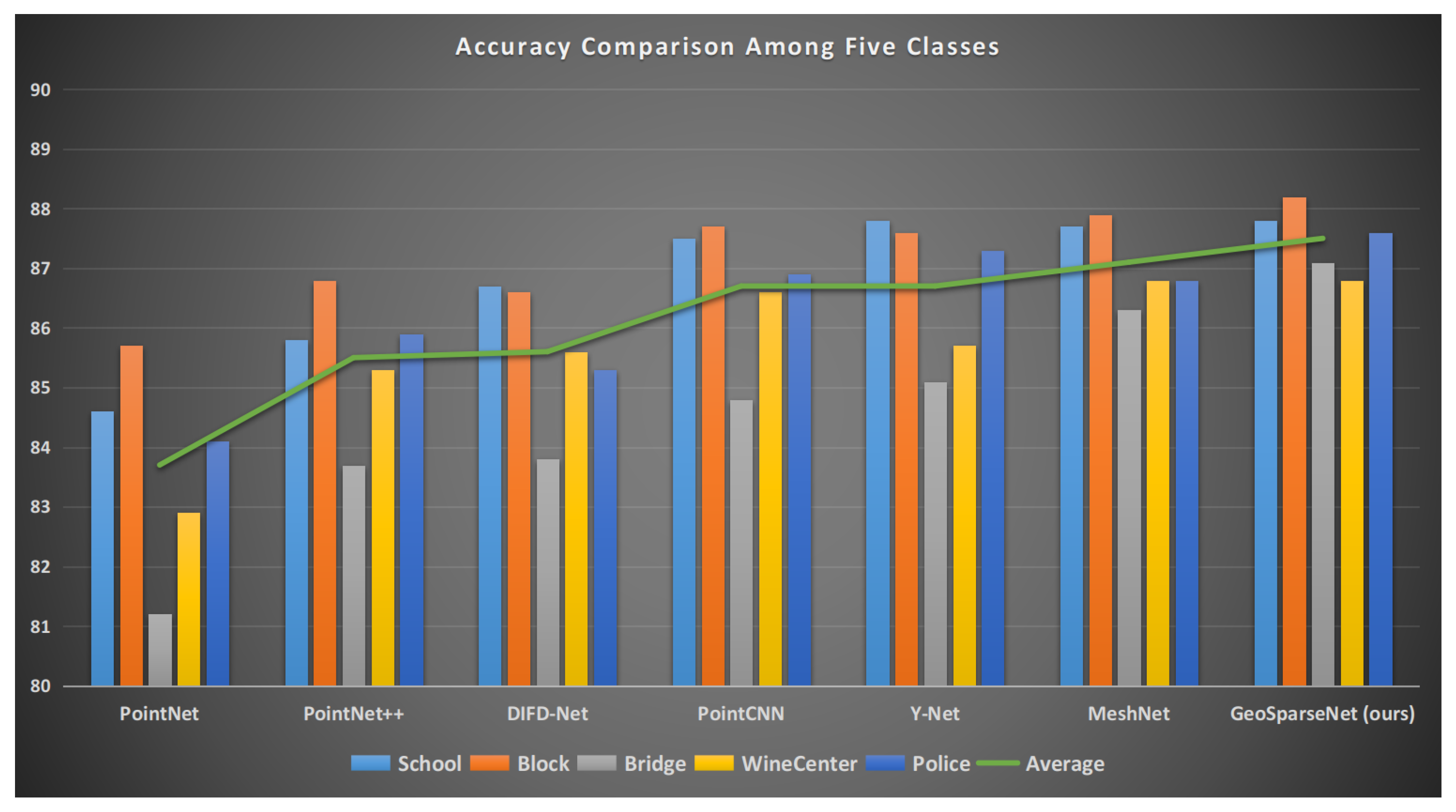
| Method | Class (%) | Average | ||||
|---|---|---|---|---|---|---|
| School | Block | Bridge | WineCenter | Police | (%) | |
| PointNet [51] | 84.6 | 85.7 | 81.2 | 82.9 | 84.1 | 83.7 |
| PointNet++ [52] | 85.8 | 86.8 | 83.7 | 85.3 | 85.9 | 85.5 |
| DIFD-Net [53] | 86.7 | 86.6 | 83.8 | 85.6 | 85.3 | 85.6 |
| PointCNN [54] | 87.5 | 87.7 | 84.8 | 86.6 | 86.9 | 86.7 |
| Y-Net [55] | 87.8 | 87.6 | 85.1 | 85.7 | 87.3 | 86.7 |
| MeshNet [56] | 87.7 | 87.9 | 86.3 | 86.8 | 86.8 | 87.1 |
| GeoSparseNet (ours) | 87.8 | 88.2 | 87.1 | 86.8 | 87.6 | 87.5 |
Disclaimer/Publisher’s Note: The statements, opinions and data contained in all publications are solely those of the individual author(s) and contributor(s) and not of MDPI and/or the editor(s). MDPI and/or the editor(s) disclaim responsibility for any injury to people or property resulting from any ideas, methods, instructions or products referred to in the content. |
© 2024 by the authors. Licensee MDPI, Basel, Switzerland. This article is an open access article distributed under the terms and conditions of the Creative Commons Attribution (CC BY) license (https://creativecommons.org/licenses/by/4.0/).
Share and Cite
Afzal, M.K.; Liu, W.; Zang, Y.; Chen, S.; Afzal, H.M.R.; Adam, J.M.; Yang, B.; Li, J.; Wang, C. GeoSparseNet: A Multi-Source Geometry-Aware CNN for Urban Scene Analysis. Remote Sens. 2024, 16, 1827. https://doi.org/10.3390/rs16111827
Afzal MK, Liu W, Zang Y, Chen S, Afzal HMR, Adam JM, Yang B, Li J, Wang C. GeoSparseNet: A Multi-Source Geometry-Aware CNN for Urban Scene Analysis. Remote Sensing. 2024; 16(11):1827. https://doi.org/10.3390/rs16111827
Chicago/Turabian StyleAfzal, Muhammad Kamran, Weiquan Liu, Yu Zang, Shuting Chen, Hafiz Muhammad Rehan Afzal, Jibril Muhammad Adam, Bai Yang, Jonathan Li, and Cheng Wang. 2024. "GeoSparseNet: A Multi-Source Geometry-Aware CNN for Urban Scene Analysis" Remote Sensing 16, no. 11: 1827. https://doi.org/10.3390/rs16111827
APA StyleAfzal, M. K., Liu, W., Zang, Y., Chen, S., Afzal, H. M. R., Adam, J. M., Yang, B., Li, J., & Wang, C. (2024). GeoSparseNet: A Multi-Source Geometry-Aware CNN for Urban Scene Analysis. Remote Sensing, 16(11), 1827. https://doi.org/10.3390/rs16111827