A Lidar Biomass Index of Tidal Marshes from Drone Lidar Point Cloud

Abstract

Accompanying climate change and sea level rise, tidal marsh mortality in coastal wetlands has been globally observed that urges the documentation of high-resolution, 3D marsh inventory to assist resilience planning. Drone Lidar has proven useful in extracting the fine-scale bare earth terrain and canopy height. Beyond that, this study performed marsh biomass mapping from drone Lidar point cloud in a S. alterniflora-dominated estuary on the Southeast U.S. coast. Three point classes (ground, low-veg, and high-veg) were classified via point cloud deep learning. Considering only vegetation points in the vertical profile, a profile area-weighted height (H_PA) was extracted at a grid size of 50 cm × 50 cm. Vegetation point densities were also extracted at each grid. Adopting the plant-level allometric equations of stem biomass from long-term S. alterniflora surveys, a Lidar biomass index (Lidar_BI) was built to represent the relative quantity of marsh biomass in a range of [0, 1] across the estuary. Compared with the clipped dry biomass samples, it achieved a comparable and slightly better performance (R² = 0.5) than the commonly applied spectral index approaches (R² = 0.4) in the same marsh field. This study indicates the feasibility of the drone Lidar point cloud for marsh biomass mapping. More advantageously, the drone Lidar approach yields information on plant community architecture, such as canopy height and plant density distributions, which are key factors in evaluating marsh habitat and its ecological services.

1. Introduction

Tidal marshes are an essential component of global coasts, at the boundary between the sea and land. The accelerating climate change, sea-level rise, and coastal development have cast great challenges on marsh vitality, which leads to wetland conversion and degraded ecological and economic services, such as nutrient filtering, storm corridors, and seafood and recreational industries [1]. On the U.S. coast, for example, the sea level is projected to rise by 10–25 inches by 2050 [2], significantly altering the current distributions of tidal marshes. A number of empirical and physical models have been developed to quantify the formation and predict the long-term dynamics of salt marshes [3]. For resilient planning utilizing these models, there is a crucial demand for 3D marsh quantification to better project marsh mortality and migration pathways in various sea level-rise scenarios.

Airborne Lidar collects sub-meter point clouds that have been successfully applied for terrestrial vegetation mapping, such as forest inventory [4]. Lidar application in tidal marshes, however, has been reportedly problematic. The Lidar-extracted marsh canopies contained high vertical uncertainties attributed to the dynamic inundation of tidal water, saturated bare earth surface, and instrument sensitivity [5,6,7,8]. Tidal marshes are characterized as grasses in relatively short forms that could not be sufficiently recorded at large spacing intervals of airborne Lidar systems. For the same reason, Lidar point clouds in marsh fields were predominantly composed of single-return points, which also turned out to underestimate the vertical marsh profiles [9].

Lidar systems onboard small unmanned aircraft systems (sUASs), or drones, could play a better role for marsh mapping in a timely manner. An sUAS is often referred to as personal remote sensing because of its flexibility in user-controlled drone flights and multi-sensor data collection. According to the current literature, drone Lidar deployment on the coast is still in its early stage. Recent studies have proven its feasibility, time, and cost efficiency on coastal mapping [10], although substantial uncertainties were observed in marsh fields [11]. In our recent study of drone Lidar deep learning [12], drone point cloud was collected at a spacing interval of 3.6 cm in an intertidal marsh field. The bare earth topography was mapped at a vertical accuracy of 5.5 cm, and the extracted marsh height had a strongly significant linear relationship with in-field measurements (Pearson’s r = 0.93). Drone Lidar systems are capable of collecting hundreds of points per square meter that are predominantly in single returns in marsh fields. With such a high point density, drone Lidar holds good potential in regard to reconstructing vegetation architecture, including plant density and marsh morphology [13], which provide useful insight into marsh’s ecological responses to sea-level rise and anthropogenic stressors.

This study explored the 3D biophysical quantities of tidal marshes from drone Lidar point cloud. As a continuous study of [12], the North Inlet estuary on the South Carolina Coast, USA, was still selected as the experimental site. Beyond the bare Earth surface and marsh height extracted from drone Lidar point clouds, this study further examined two key variables describing a marsh’s plant community architecture that led to a Lidar biomass index. The approaches proposed in this study provided useful insights for operational application of drone Lidar systems for quantitative marsh mapping, ecological surveying, and coastal resilience planning.

2. Study Area and Methods

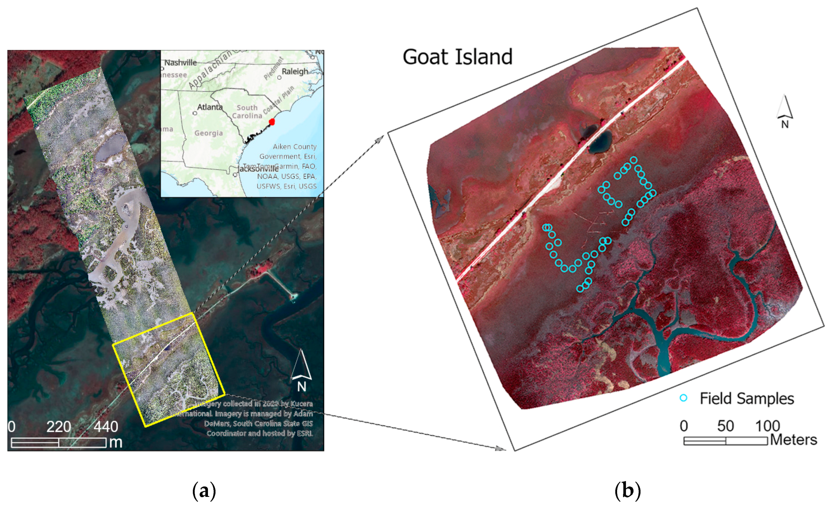
2.1. Study Area and Field Experiments

The North Inlet in Georgetown, South Carolina (Figure 1), is a high-salinity ocean-dominated estuary in a largely undeveloped watershed dominated by native smooth cordgrass, S. alterniflora throughout of the intertidal area [14]. The S. alterniflora zone of salt marshes on the U.S. West Coast can be split into two ecological habitats relative to tidal inundation and plant morphology: low marshes (tall plant forms) in the regularly flooded estuary below the mean high water (MHW) and high marshes (short plants) in areas above the MHW [15]. The estuary contains numerous shallow creeks and intertidal mudflats inundated by semidiurnal tides with a mean diurnal tidal level (the difference between MHW and mean low water) of 0.8 m according to the datum at the nearby NOAA Station (8662288, Clambank Creek Dock). Therefore, S. alterniflora in the estuary grows in both low marsh and high marsh forms upon its relative topography.

The study site in the estuary, centered at (33°20′02.06”N, 79°11′44.40”W), was referred to as Goat Island in this study (Figure 1a). It has a flat topography gradually decreasing from the northwest (roadside) to southwest (interior estuary). Marshes in the study site are characterized by the single species of S. alterniflora, commonly referred to as a Spartina monoculture. In the middle of the orthoimage (Figure 1b) are some boardwalks permanently built for the NSF Long-Term Research in Environmental Biology (LTERB) project at North Inlet. Along these boardwalks, a number of 1.5 m × 1.5 m plots have been established for experimentally fertilizing S. alterniflora to test its responses to added nitrogen and phosphorus [16].

On 31 August 2022, the drone lidar mission was operated in a spirograph scanning mode on a long strip passing Goat Island in a daytime, low-tide window. The Lidar system was Livox Avia (ROCK Robotic, Denver, CO, USA) onboard DJI Matrice 300 RTK (SZ DJI Technology Co. Ltd., Shenzhen, China). At a flight altitude of 80 m above ground, the collected point cloud reached a spacing interval of 3.6 cm with 600–800 points per square meter. On 21 September 2022, a drone photogrammetry mission was deployed to collect multispectral imagery using the MicaSense RedEdge-M camera (AgEagle Aerial Systems Inc., Wichita, KS, USA) onboard Matrice 100. The flights were made at the same altitude as the drone Lidar, covering the southern end of the Lidar strip. The drone imagery package was processed in the Pix4DMapper software (Pix4D S.A., Lausanne, Switzerland) to produce the surface-reflectance orthoimage in five spectral bands: blue, green, red, near infrared (NIR), and red edge. The normalized difference vegetation index (NDVI) was then extracted and served as an example of spectral methods for marsh biomass estimation to be compared with the Lidar method in this study. Similarly, this mission was launched in a daytime low-tide window.

Finally, in a multi-day campaign on 21–24 September 2022, in-field samples of S. alterniflora were collected at Goat Island. In a 0.5 m × 0.5 m quadrat at each sample point, the marsh canopy height was collected from five randomly selected plants, and all marsh plants were clipped and dried to measure dry biomass (g/m²). The campaign collected 40 sample points across the study area. In general, S. alterniflora at North Inlet reaches its peak growth in September [17]. We assumed that the temporal variation in biomass in the three experiments was not significant.

2.2. Previous Work

Deep learning of the collected drone Lidar point cloud at Goat Island was explored in our previous study [12] to classify the mass points into ground (Code #2), low vegetation (Code #3, hereafter referred to as low-veg), and high vegetation (Code #5, hereafter referred to as high-veg) under the ASPRS LAS Specification V1.4 Standard. The ground points represented bare earth. The high-veg points were on the top layer of the point profile, revealing apparent canopy structures of the tall-form marsh plants. The low-veg points were the short-form plants above ground or those below the high-veg points in the point profile. According to the validation set, the harmonic accuracies of ground, low-veg, and high-veg reached 0.88, 0.86, and 0.80, respectively. The ground points had the best performance with balanced precision and recall values. The low-veg and high-veg points turned out to be misclassified by being assigned to each other in the high marsh/low marsh transitional zones. The misclassification was reasonable because there is no clear morphological delineation between the two marsh forms of S. alterniflora. This study directly utilized the classified drone Lidar point cloud at Goat Island.

2.3. Approaches

2.3.1. Extracting Plant Structures from Lidar Point Cloud

The Digital Surface Model (DSM) was extracted as the top envelop, and the Digital Terrain Model (DTM) was the bottom envelop of the point cloud. Given the 3.6 cm spacing of the drone Lidar point cloud in this study, a grid size of 10 cm was selected to as the unit of the DSM and DTM raster layers. The marsh height at each grid was simply the vertical difference between DTM and DSM surfaces. The extracted 10 cm marsh height map provides a fine-scale representation of the maximal height of marsh plants.

Aside from marsh height, Lidar point density may also play a role in quantifying marsh biomass. Marsh plants have relatively sparse leaf distributions. Past studies found that both airborne [9] and drone [12] Lidar point clouds had predominantly single returns in marsh environments. Therefore, the density of vegetation points may bear certain relationships with the plant density in a marsh field. The vegetation point density in a grid cell is the total number of vegetation points within this grid. Different from the finer scale (10 cm grid) for marsh height mapping, a 50 cm grid size was used for fair representation of marsh plant densities in the field.

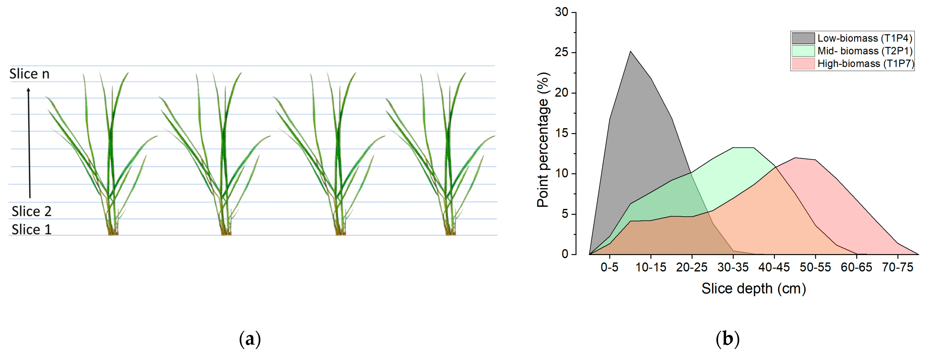
2.3.2. A Profile Area-Weighted Height

S. alterniflora marshes in the study area grow in a relatively homogeneous grassland that varies in biomass and canopy height as a function of environmental conditions such as topography, tidal flooding, and sediment nutrient content. Three field samples were selected to demonstrate marshes in low, medium, and high biomass levels (

Table 1. Example marsh samples in different biomass levels.

	Bare-Earth Elevation (m)	Biomass (g/m2)	In-Field Marsh Height (m)	Lidar Marsh Height (m)	Total Point Density (/m2)
T1P4	0.41	274.19	0.42	0.26	656
T2P1	0.24	335.23	0.99	0.55	704
T1P7	0.10	591.41	1.31	0.72	596

). Their elevations were measured in the North American Vertical Datum 1988. Note that these three examples showed a trend of increasing biomass from higher to lower elevations. The total point densities of Lidar point cloud were similar among the three samples because of the single-return characteristics in marsh fields. It also deserves to be mentioned that the Lidar-extracted marsh height was dramatically lower than in-field measurements, but the two variables held a strong linear relationship. More details about marsh height mapping were described in [12].

As demonstrated in Figure 2a, slicing the point cloud at a certain depth interval, the point percentage at each depth can be measured at a 50 cm × 50 cm grid, and the point percentage profile of this grid can be extracted (Figure 2b). The three field samples (T1P4, T2P1, and T1P7) in the figure demonstrate that the distributions of point percentage profiles vary at different biomass levels. The profile of the low-biomass sample (T1P4) has a low peak, meaning the dominant Lidar points at this sample are located closer to ground. Oppositely, the profile at high biomass (T1P7) has a much higher peak, indicating that its dominant Lidar points are much higher. Figure 2 indicates that the profile areas of vegetation point percentages may contribute to quantifying marsh biomass.

Based on the point percentage profile, this study proposes a new variable, the profile area-weighted height (H_PA), to represent the statistically averaged marsh canopy height. A marsh field is divided into n slices at a given depth, S_depth. The number of slices is determined by the Lidar-extracted maximal marsh height, $H_{max}$:

$$n=int\left(\frac{H_{max}}{S_{depth}}\right)$$

(1)

At each slice depth i, we can extract the number of points in this slice and its point percentage, $f_i$, against the total vegetation points. The H_PA at this grid can be calculated as follows:

$$H_{PA}=\frac{\sum _{i=2}^n{f}_i\times S_{depth}}{1-f_1}$$

(2)

where $f_1$ is the point density at the first slice. This slice holds inevitable noises from misclassified ground points, litter, and other non-foliage points on bare earth surface. To reduce the noise, points in this first slice are not counted. A depth of 3 cm was selected in this study.

2.3.3. Lidar Biomass Index (Lidar_BI)

Marsh biomass, productivity and its ecological functions at the North Inlet estuary have been intensively studied in past efforts, such as the NSF Long-Term Research in Environmental Biology (LTERB) project. Utilizing multi-year (>5 years) ground measurements, the allometric equations for S. alterniflora were established [16]. By censusing the stem heights of all marsh plants at permanent LTERB plots on a monthly basis and comparing with each plant’s stem dry mass (g/plant) from destructive harvesting measurements, a set of time-variant marsh morphology-related polynomial (2nd order or higher) relationships were established between the stem height and the mass of a single marsh plant. In this study, we adopted these allometric equations to estimate the plant-level stem biomass from the Lidar-extracted H_PA at the 40 field samples. Assuming H_PA to be the stem height, the allometric equation describes the stem biomass as follows [16]:

$${Bio}_{stem}=a_0+a_1\times H_{PA}+a_2\times H_{PA}^2$$

(3)

where ${Bio}_{stem}$ is the plant-level stem biomass (g/plant). The H_PA has a unit of cm.

In Equation (3), different sets of coefficients are used in each month, which also vary in tall and short marsh forms. Given the drone Lidar flights on 31 August, we adopted the equations for the month of September. A threshold of H_max = 1.0 m was used to delineate short-form and tall-form marsh plants of all samples at Goat Island. The calculations were made in the Plant Weight Calculator tool, as described in [16].

The biomass density in a grid unit is the multiplication of plant-level stem biomass and number of plants per unit area. This study could not directly calculate the biomass density (g/m²) from stem biomass because vegetation point density is not a measure of the stem density of plants. Rather, the Lidar point density at a grid cell varies with sensor, flight height, and scanning mode. Thanks to the single-return feature of Lidar point cloud in marsh fields, marshes with more vegetation points fairly indicate higher stem densities. Given a 50 cm × 50 cm grid cell, this study proposes a Lidar biomass index:

$$Lidar\_BI={Bio}_{stem}\times N_{veg}/scale$$

(4)

where $N_{veg}$ is the total number of vegetation points of the grid cell. The term scale is a numeric factor to re-scale biomass density into [0, 1], which is determined to be the 0.5% right tail of its distributions at Goat Island.

The $Lidar\_BI$ serves as a biomass indicator. Although it does not directly measure the dry biomass quantities as the harvest approaches, it reasonably indicates the relative marsh abundance across the field.

3. Results and Discussion

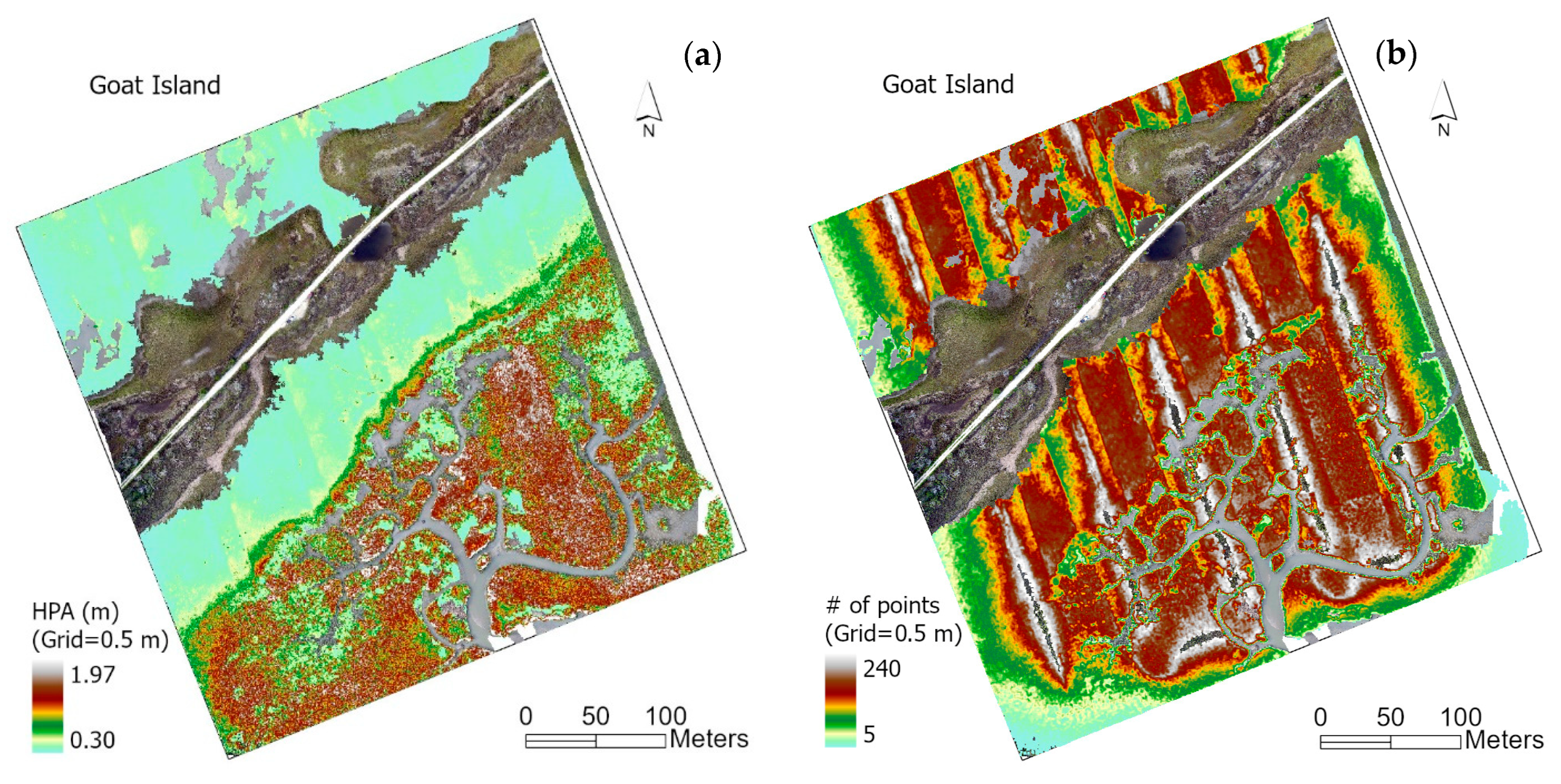
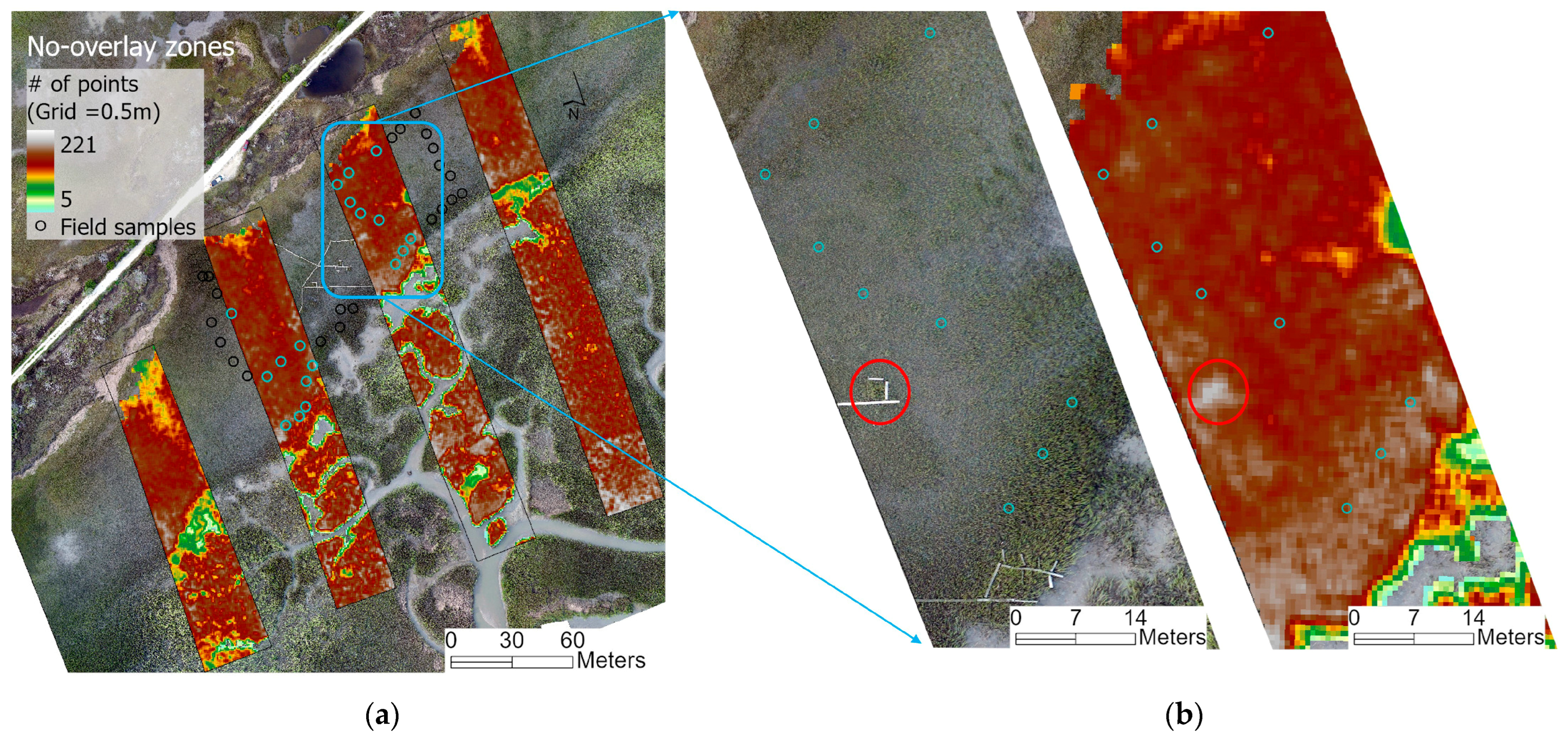
3.1. Classified Point Cloud and Marsh Characteristics

As shown on the drone orthoimage (Figure 3a), the study site is dominated by intertidal marshes expanding from the roadside to the interior estuary. Isolated trees and shrubs grow along the road. The Lidar system deployed in this study has the capacity of three returns in maximum from each illuminated laser beam. Statistically, 99.7% of Lidar points at the study area were the first returns, 0.29% the second returns, and 0.01% the third (and last) returns. The second and third returns are overlaid on the orthoimage in Figure 3a. Most of these returns were from trees and shrubs along the road. In marsh fields, these second and third returns were limited, only scattering along the edge of tidal channels.

Three point classes in marsh fields (ground, low-veg, and high-veg) were classified from the Lidar point cloud. Their spatial distributions reflected the landscape of intertidal wetlands (Figure 3b). The Spartina monoculture in the study area contains two marsh forms, i.e., low marsh dominated by tall-form S. alterniflora in the interior estuary below MHW, and high marsh represented by short-form S. alterniflora above MHW. In Figure 3b, low-veg (dark green) and high-veg (light green) points reveal the geographic patterns of the two marsh forms, showing a distinctive cutline between low marsh and high marsh zones. The roadside trees and shrubs reveal clear canopy structures in the Lidar point cloud. Figure 3c is an example point cloud profile along a transect from roadside to tidal creek. In this profile, ground points are identified at the bottom, low-veg points above ground, and high-veg points are above low vegetation, especially in tall-form marshes in the interior estuary.

3.2. Lidar-Extracted Marsh Heights and Densities

3.2.1. The Maximal Marsh Height ($H_{max}$) and Total Point Density

The Lidar-extracted marsh height ($H_{max}$) raster represented the maximal plant height at each 10 cm × 10 cm grid. Wang et al. [12] reported a significant and strong linear relationship (Pearson’s r = 0.93) between the Lidar-extracted marsh height and in-field measurements. In this study, we applied the linear relationship to adjust the Lidar-extracted marsh height to the level of in-field marsh height. Hereafter, $H_{max}$ is referred to as the adjusted Lidar-extracted maximal plant height.

Similar to the classified Lidar point cloud in Figure 3b above, the $H_{max}$ map in Figure 4a reveals a clear transition between high marsh and low marsh forms. According to our field experiences and knowledge on coastal wetlands, marsh plants rarely exceed 2 m. The marsh height map in Figure 4a is truncated at 2 m. The minimal marsh height that can be extracted from Lidar point cloud was 0.2 m. The histogram of $H_{max}$ in Figure 4b shows the dominancy of shorter marsh plants at Goat Island. This is reasonable because it is located at the landward edge of the estuary (as shown in Figure 1a). The mean $H_{max}$ was 0.73 m, with 84% of pixels falling below 1.2 m and 95% below 1.63 m. Be aware that the sample points were located at the higher elevations of the marsh platform; the lower elevation vegetation could not be sampled due to the difficulty to access the more unconsolidated marsh sediment at these elevations. Caution should thus be taken in interpretating those exceptionally tall marsh plants.

The total point density was extracted at a grid size of 50 cm (Figure 4c). For sUAS missions, there are always overlap zones between two adjacent flight lines, in which Lidar points from both flight lines are collected. Therefore, more points are recorded in the overlap zones than in regular flight areas. In Figure 4c, the excessive points in the overlap zones are visually apparent. In a spirograph scanning mode, the overlap points were concentrated along the central line and rapidly decayed toward the edge of the overlap zone. Goat Island was located at the end of the flight strip. At its south end, the bright semicircular curves indicated the flight transition between two adjacent flight lines. Except for these overlaps, there was a relatively homogeneous distribution of total point densities because of the Spartina monoculture at Goat Island.

During a drone Lidar mission, the scan angles of points from different flight lines may vary widely. The attribute of point source ID for each flight line is often recorded in drone Lidar missions. In the overlap zones where both records of point source ID are available, points with the scan angles farther away from nadir can be recognized as overlap points [18]. In the drone missions of this study, unfortunately, these system factors were not recorded. The overlap points could not be recognized and filtered out. The overlap points cast a strong impact on the extracted point densities. At Goat Island, the Lidar points reached up to 630 points per 50 cm × 50 cm grid, with an average of 138 points per grid (Figure 4d). The high densities in the right tail of the histogram were from the overlap points especially in the central overlap zones (bright pixels in Figure 4c). If these overlap noises were not considered, the total point density had a relatively normal distribution (Figure 4d), which reasonably represented the point densities in a marsh field.

3.2.2. Profile Area-Weighted Height ($H_{PA}$) and Vegetation Point Density (N_veg)

The H_PA within a 50 cm × 50 cm grid was a statistically weighted height of all marsh vegetation points based on the point percentages of slices at a 3 cm depth. At Goat Island, the H_PA ranged from 0.3 m roadside to around 2 m in the interior estuary (Figure 5a). Similar to the $H_{max}$, the H_PA had an increasing trend from the roadside to the interior marshes, which was in good agreement with the bio-properties of S. alterniflora in the estuary. Similarly, there was a distinctive split line between two marsh forms at Goat Island.

For marsh vegetation point density, pixels falling in the ±5% tails of the histogram were not mapped in order to reduce the impact of noises especially the overlap points. The resulting vegetation point density map at Goat Island had a range of [5, 240] points in the 50 cm grid size (Figure 5b). Areas in high densities (in white) were the overlap points distributed along the central overlap zones. Be aware that the Goat Island site was located at the south end of the flight footprint. The exceptionally low densities along the flight edges may come from system noises.

Vegetation point densities in the non-overlap zones reflected more useful information about plant densities in the field. The four non-overlap zones (Figure 6a) were extracted. Among the 40 field samples marked in the figure, 18 were in these non-overlap strips. At such a fine scale, this marsh field revealed subtle variations in point densities spatially. Vegetation point densities were lower at the roadside.

As better demonstrated in a subset area, or the LTERB field in Figure 6b, there are higher point densities (in light gray) along the creek banks where marshes transit from short-form to tall-form marsh habitats. One LTERB plot (marked in a red circle) is visible on the orthoimage in Figure 6b. It was fertilized and therefore had taller plants [12]. As reflected in the vegetation density map, this plot also has much higher plant density than naturally grown marshes nearby. Figure 6 reveals that the Lidar-extracted vegetation point density could play a role in indicating plant density in marsh fields.

3.3. Lidar-Extracted Marsh Biomass Index and Comparison with the Spectral Method

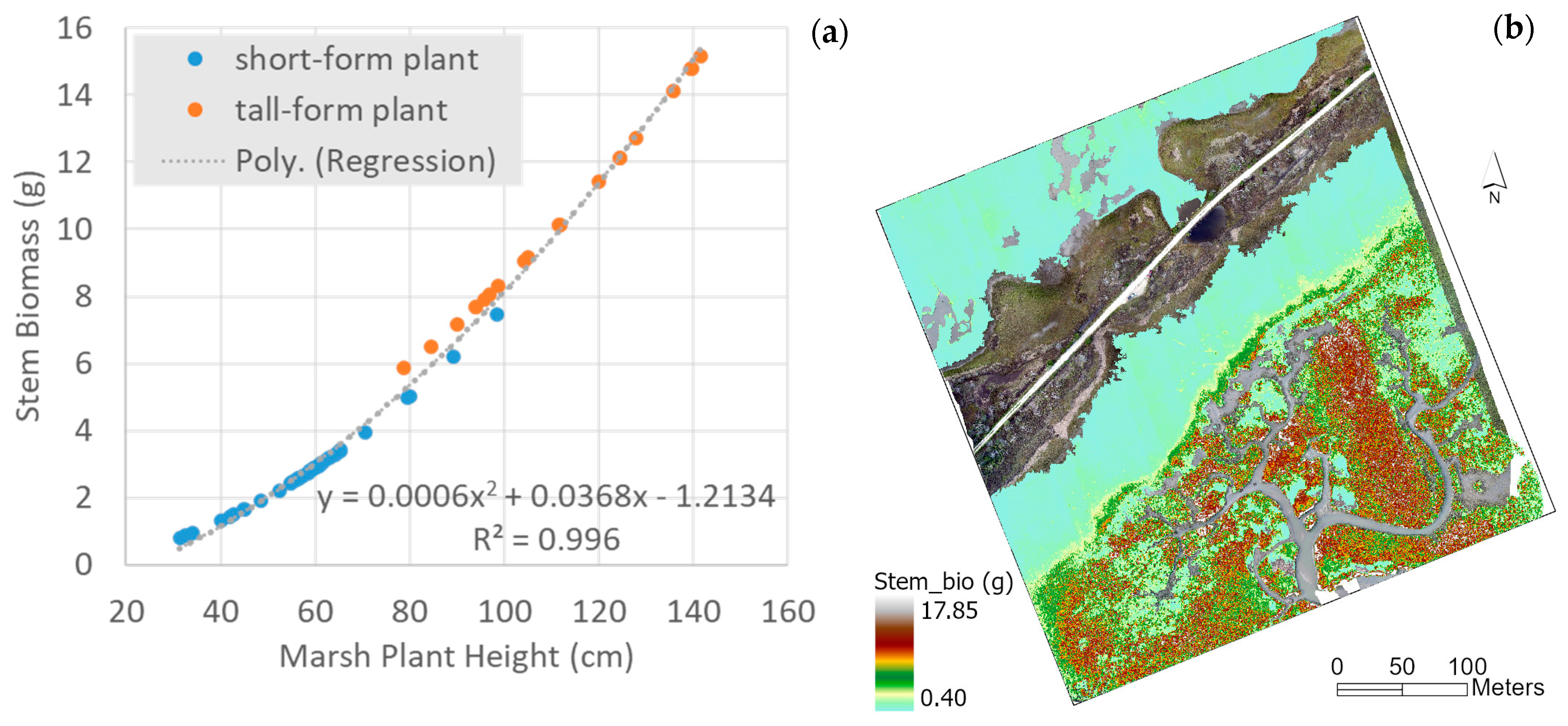
3.3.1. Plant-Level Stem Biomass (${Bio}_{stem}$)

Applying the Plant Weight Calculator [16] for short-form and tall-form plants, the stem biomass at all sample points was modeled with the Lidar-extracted H_PA (Figure 7a). Plants in the height range of 80–100 cm were calculated in both forms. Although the two allometric equations did not perfectly converge, when all samples at Goat Island were considered, there was still a strong second-order polynomial relationship between H_PA and the stem biomass, with R² = 0.996. The coefficients of the regression model are described in Figure 7a. Using this regression model, the stem biomass (${Bio}_{stem}$) was mapped at the study site (Figure 7b). To reduce the visual impact of outliers in the color legend, the ${Bio}_{stem}$ pixels in the 0.5% right tail (>17.85 g/plant) are truncated.

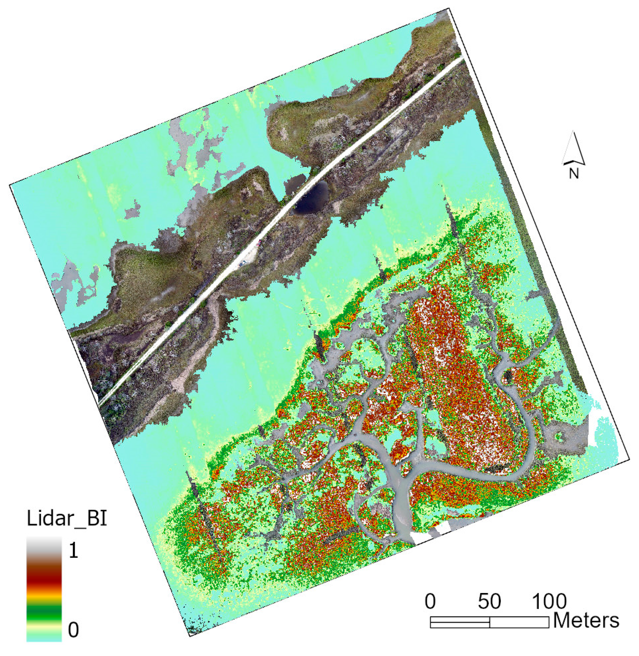
3.3.2. Lidar Biomass Index (Lidar_BI)

The Lidar biomass index was calculated using Equation (4). The 0.5% right tail of the ${Bio}_{stem}\times N_{veg}$ histogram at Goat Island was 2933.44. A scale factor of 3000 was therefore selected. The resulting Lidar_BI was a ratio index in the range of [0, 1] to represent relative marsh biomass across the field (Figure 8). Similarly, the no-marsh fields and marshes with extreme overlap points were masked out. The Lidar_BI distributions at Goat Island agreed with our common understanding of S. alterniflora landscapes (Pennings and Bertness 2001), i.e., biomass was much lower above MHW and higher in the interior estuary below MHW. The Lidar_BI was still affected by the overlap points, revealing certain linear patterns, especially in the low biomass zones at the roadside. The impact of overlap points on biomass index, however, was less dramatic than that on vegetation density (Figure 5b). Overall, Figure 8 reflects the fine-scale biomass dynamics in marsh fields.

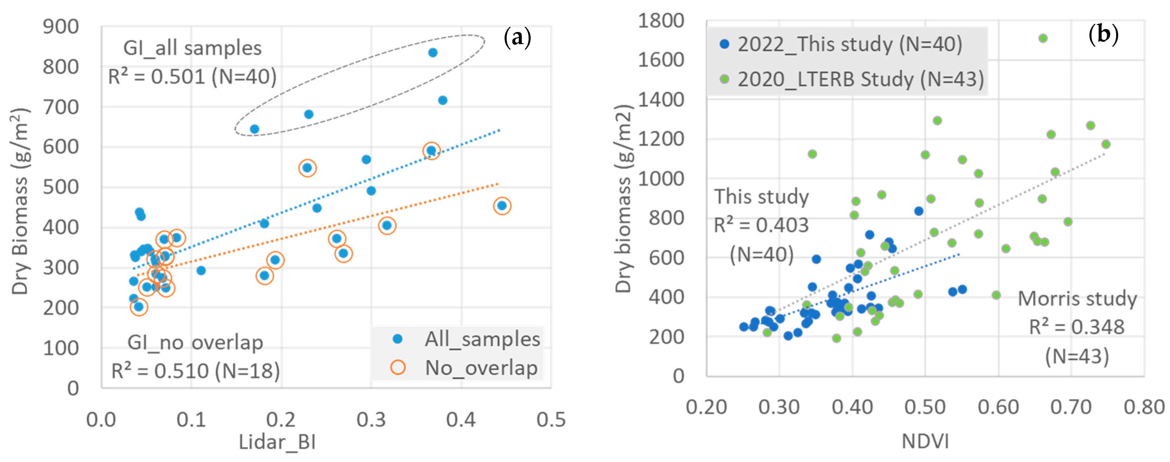
3.3.3. Comparison between the Lidar_BI and the NDVI Methods for Biomass Estimation

A linear relationship was observed between Lidar_BI and the clipped dry biomass at the sample points (Figure 9a). The R² reached 0.50 when all of the 40 samples were considered and was slightly higher (0.51) with merely the 18 sample points located in non-overlap areas. Although the two relationships were not statistically significant, the non-overlap scatterplot revealed less deviation from the regression line. As marked in Figure 9a, three of four high-biomass samples (>600 g/m²) turned out to be poorly matched. Their in-field marsh heights were around 100–108 cm, and the Lidar-extracted H_max values were 94–136 cm, belonging to the tall-form plants at Goat Island. Except for these three samples, other tall-plant samples with a similar marsh height had much lower dry biomass, and, therefore, their Lidar_BI matched better with the clipped dry biomass. Be aware that this study sampled a marsh field that was closer to a road. Further investigation is needed in interior marsh fields with taller plants.

Our Lidar method was also compared with the spectral methods of marsh biomass estimation. Optical remote sensing has been popularly applied to estimate marsh biomass based on the spectral properties of healthy vegetation. A number of studies of S. alterniflora have reported linear relationships between its dry biomass and vegetation index (e.g., NDVI), with R² in a range of 0.3–0.6 depending on sensors, image resolutions, environment conditions, sample sizes, etc. [17,19,20]. As a test experiment of this study, the NDVI values at the field samples were extracted from the drone-collected RedEdge-M surface reflectance imagery (see Figure 1). At the same 40 sample points, the NDVI-based dry biomass regression had a R² = 0.403 that agreed with past studies (Figure 9b).

The NDVI-biomass regression from multispectral imagery is subject to temporal dynamics. Even in peak growing seasons, biophysical properties of marsh plants with the same biomass may vary greatly in different years due to the changing conditions of weather, solar illumination, and phenological development. Figure 9b also includes an independent sample set collected on a monthly basis at the LTERB plots on Goat Island. On 15 August 2020, biomass records at 43 LTERB subplots (10 cm × 15 cm each) were surveyed in previous projects [16]. On 30 August 2020, the DJI Matrice 100/RedEdge-M drone system was deployed at the same flight configuration as this study. The NDVI values at the surveyed LTERB subplots were extracted from the calibrated RedEdge-M surface reflectance image. As shown in Figure 9b, both NDVI and biomass quantities in the LTERB subplots are generally higher than those in non-managed marshes collected in this study. The deviations from the regression line were also higher, resulting in a lower R² = 0.348. Figure 9b reveals that the empirical NDVI-based biomass estimation could vary dramatically in different case studies.

Different from the NDVI method, the Lidar_BI is a semi-allometric approach that measures the vertical structure instead of the spectral properties of marsh plants. Radiometric calibration and atmospheric correction are a prerequisite in the NDVI method, but they are not needed in Lidar remote sensing. The per-plant allometric relationships of S. alterniflora are also temporally dynamic, possibly as a function of nutrient levels, weather conditions, etc. However, the Lidar-extracted plant height and density directly contribute to aboveground biomass measurement. In this sense, the Lidar method is less sensitive to the influence of environmental variabilities than the NDVI method. However, it should be noted that the Lidar_BI algorithm depends on the allometric relationships between plant height and stem biomass that also vary with the marsh species, growing season, geography. This study adopted the allometric equations that were specifically developed for the S. alterniflora community in the North Inlet Estuary. Morris [21] compared two S. alterniflora communities between the North Inlet Estuary at SC (same as this study) and Plum Island Estuary at MA, in which significantly different allometric equations were extracted. When applying the Lidar_BI algorithm in other drone Lidar missions, the coefficients of the allometric equations need to be empirically justified in site-specific marshes.

3.4. Drone Lidar for 3D Marsh Mapping: Pros and Cons

Tidal marshes have relatively low biomass, short canopy heights, and homogeneous structures in comparison with terrestrial ecosystems like forests. Past studies have reported the insufficiency of airborne Lidar applications for tidal marsh mapping [7]. While drone Lidar deployment in coastal wetlands is still in its early stage, recent studies have revealed its advantages in extracting bare earth surfaces and marsh height that were superior to airborne Lidar [12,13]. The 3D marsh canopies extracted from drone Lidar point cloud jointly contributed to marsh biomass quantification.

More advantageously, flying at a lower altitude, drone Lidar could collect hundreds of points per square meter instead of 2–3 points from airborne Lidar. Dense points of marsh canopies allow for the statistical measurement of the marsh canopy height in unit grids (e.g., 50 cm × 50 cm in this study). This study proposed a profile area-weighted height (H_PA) to measure the statistical average of canopy height weighted by point densities in incremental slice depths. It is a more reasonable representation of plant vertical structure in the grid than the maximal height extracted from the topmost Lidar points. It allows for estimates of small-scale patterns of canopy-structure architecture (density and height distributions) that has been shown to be critical to marsh’s ecological functions on trapping sediments and accreting with sea-level rise [22]. It this sense, drone Lidar holds great potential for investigating ecological importance of intertidal marshes.

For operational drone Lidar applications, the overlap points in two adjacent flight paths need to be better examined. In this experimental study, the scan angles and source IDs (flight paths) of Lidar points were not recorded. The overlap points thus could not be delineated in common Lidar point cloud software packages. The overlap points did not significantly affect the extraction of marsh height. However, the excessive points in the overlap zones resulted in higher vegetation point density that turned to overestimate marsh biomass. In future drone Lidar missions, rigid flight configuration should be carried out so that the overlap points could be effectively removed for advanced 3D marsh mapping.

The proposed Lidar_BI in this study is a ratio index in a range of [0, 1] to represent relative marsh biomass. As a semi-allometric approach, it calculates the grid-level marsh biomass by integrating the stem biomass (per plant) and vegetation point density in the grid weighted by point heights at different slice depths. The scale factor in the Lidar_BI equation is data dependent (Lidar sensor, scanning mode, flight height, etc.), but it can be statistically determined from the collected Lidar point cloud. Past studies found that the Lidar-extracted marsh height was lower than the in-field measured marsh height; however, a strongly linear relationship (Pearson’s r = 0.925) was observed [12]. This study applied the linear model to project the Lidar-extracted marsh height to in-field height. This empirical model, however, was built on marsh samples with relatively shorter plants and lower biomass in an S. alterniflora community. In future research, the tall-form marshes in an interior estuary need to be sampled for a comprehensive evaluation of the proposed Lidar_BI approach.

This study is among the frontier efforts of marsh biomass mapping with drone Lidar observations. The Lidar_BI provides spatially explicit information of marsh canopy architecture and relative biomass in intertidal zones. With accelerated climate change and sea-level rise, tidal marsh mortality and coastal sustainability have been under deeper investigation. Taking advantage of drone Lidar deployment, the fine-scale 3D marsh information is essential in modeling marsh migration and wetland conversion in various scenarios of sea-level rise.

4. Conclusions

This study performed 3D marsh mapping from Lidar point cloud in an ocean-front pristine estuary. Three point classes (ground, low-veg, and high-veg) in an S. alterniflora field were classified via deep learning of Lidar point cloud. Slicing the vertical profile of vegetation point cloud at a 3 m depth, the profile-area weighted marsh canopy height (H_PA) was extracted at a grid size of 50 cm × 50 cm. Relying on long-term S. alterniflora surveys and the established allometric equations of per-plant stem biomass, a Lidar biomass index (Lidar_BI) was proposed to represent the relative quantity of marsh biomass in the estuary. The primary findings of this experimental study include the following:

• Similar to airborne Lidar systems, drone Lidar point cloud is characterized by single returns in tidal marshes.
• The H_PA better describes the biophysical properties of marsh fields than the maximal marsh height extracted from the topmost Lidar points.
• The semi-allometric ratio index, Lidar_BI, represents relative marsh biomass in a spatial dimension. For quantitative biomass estimation, it achieves a comparable and slightly better performance (R² = 0.5) than the commonly applied vegetation index approach.

This study indicates the feasibility of drone Lidar for marsh biomass assessment, which could be a favorable alternative to multispectral imagery, on which a marsh’s spectral properties vary dramatically according to the solar illumination conditions. For practical drone Lidar applications, further investigation is needed to remove the overlaid points between two flight lines.

References

1. Sanger, D.; Parker, C. Guide to the Salt Marshes and Tidal Creeks of the Southeastern United States; South Carolina Department of Natural Resources: Barnwell, SC, USA, 2016; 112p.
2. Sweet, W.V.; Hamlington, B.D.; Kopp, R.E.; Weaver, C.P.; Barnard, P.L.; Bekaert, D.; Brooks, W.; Craghan, M.; Dusek, G.; Frederikse, T.; et al. Global and Regional Sea Level Rise Scenarios for the United States: Updated Mean Projections and Extreme Water Level Probabilities Along U.S. Coastlines; NOAA Technical Report NOS 01; NOAA National Ocean Service: Silver Spring, MD, USA, 2022; 111p.
3. Fagherazzi, S.; Kirwan, M.L.; Mudd, S.M.; Guntenspergen, G.R.; Temmerman, S.; D’Alpaos, A.; Van De Koppel, J.; Rybczyk, J.M.; Reyes, E.; Craft, C.; et al. Numerical models of salt marsh evolution: Ecological, geomorphic and climatic factors. Rev. Geophys. 2011, 50, RG1002. [Google Scholar] [CrossRef]
4. Reutebuch, S.E.; Andersen, H.E.; McGaughey, R.J. Light detection and ranging (lidar): An emerging tool for multiple resource inventory. J. For. 2005, 103, 286–292. [Google Scholar] [CrossRef]
5. Schmid, K.A.; Hadley, B.C.; Wijekoon, N. Vertical accuracy and use of topographic Lidar data in coastal marshes. J. Coast. Res. 2011, 27, 116–132. [Google Scholar] [CrossRef]
6. Hladik, C.; Alber, M. Accuracy assessment and correction of a Lidar-derived salt marsh digital elevation model. Remote Sens. Environ. 2012, 121, 224–235. [Google Scholar] [CrossRef]
7. Amante, C. Estimating coastal digital elevation model uncertainty. J. Coast. Res. 2018, 34, 1382–1397. [Google Scholar] [CrossRef]
8. Medeiros, S.C.; Bobinsky, J.S.; Abdelwahab, K. Locality of topographic ground truth data for salt marsh Lidar DEM elevation bias mitigation. IEEE J. Sel. Top. Appl. Earth Obs. Remote Sens. 2022, 15, 5766–5775. [Google Scholar] [CrossRef]
9. Fernandez-Nunez, M.; Burningham, H.; Ojeda Zujar, J. Improving accuracy of Lidar-derived terrain models for saltmarsh management. J. Coast Conserv. 2017, 21, 209–222. [Google Scholar] [CrossRef]
10. Pinton, D.; Canestrelli, A.; Wilkinson, B.; Ifju, P.; Ortega, A. A new algorithm for estimating ground elevation and vegetation characteristics in coastal salt marshes from high-resolution UAV-based Lidar point clouds. Earth Surf. Process. Landf. 2020, 45, 3687–3701. [Google Scholar] [CrossRef]
11. Blount, T.; Silvestri, S.; Marani, M.; D’Alpaos, A. Lidar derived salt marsh topography and biomass: Defining accuracy and spatial patterns of uncertainty. Int. Arch. Photogramm. Remote Sens. Spat. Inf. Sci. 2023, 48, 57–62. [Google Scholar] [CrossRef]
12. Wang, C.; Morgan, G.R.; Morris, J.T. Drone Lidar deep learning for fine-scale bare earth surface and 3D marsh mapping in intertidal estuaries. Sustainability 2023, 15, 15823. [Google Scholar] [CrossRef]
13. Pinton, D.; Canestrelli, A.; Wilkinson, B.; Ifju, P.; Ortega, A. Estimating ground elevation and vegetation characteristics in coastal salt marshes using UAV-based Lidar and digital aerial photogrammetry. Remote Sens. 2021, 13, 4506. [Google Scholar] [CrossRef]
14. Allen, D.M.; Allen, W.B.; Feller, R.F.; Plunket, J.S. (Eds.) Site Profile of the North Inlet-Winyah Bay National Estuarine Research Reserve; North Inlet-Winyah Bay National Estuarine Research Reserve: Georgetown, SC, USA, 2014; 432p. [Google Scholar]
15. Pennings, S.C.; Bertness, M.D. Salt marsh communities. In Marine Community Ecology; Bertness, M.D., Gaines, S.D., Hay, M.E., Eds.; Sinauer Associates: Sunderland, MA, USA, 2001; pp. 289–316. [Google Scholar]
16. Morris, J.; Sundberg, K. LTREB: Aboveground Biomass, Plant Density, Annual Aboveground Productivity, and Plant Heights in Control and Fertilized Plots in a Spartina Alterniflora-Dominated Salt Marsh, North Inlet, Georgetown, SC: 1984–2020; Ver 5; Environmental Data Initiative: Albuquerque, NM, USA, 2021. [Google Scholar] [CrossRef]
17. Miller, G.J.; Morris, J.T.; Wang, C. Estimating Aboveground Biomass and Its Spatial Distribution in Coastal Wetlands Utilizing Planet Multispectral Imagery. Remote Sens. 2019, 11, 2020. [Google Scholar] [CrossRef]
18. ESRI 2023. ArcGIS Pro 3.2—Understand Overlap Classification. Available online: https://pro.arcgis.com/en/pro-app/latest/help/analysis/3d-analyst/overlap-workflow.htm (accessed on 16 February 2024).
19. Jensen, J.R.; Coombs, C.; Porter, D.; Jones, B.; Schill, S.; White, D. Extraction of smooth cordgrass (spartina alterniflora)biomass and leaf area index parameters from high resolution imagery. Geocarto Int. 1998, 13, 25–34. [Google Scholar] [CrossRef]
20. Doughty, C.L.; Cavanaugh, K.C. Mapping Coastal Wetland Biomass from High Resolution Unmanned Aerial Vehicle (UAV) Imagery. Remote Sens. 2019, 11, 540. [Google Scholar] [CrossRef]
21. Morris, J.T. Estimating net primary production of salt-marsh macrophytes. In Principles and Standards for Measuring Primary Production; Fahey, T.J., Knapp, A.K., Eds.; Oxford University Press: Oxford, UK, 2007; pp. 106–119. [Google Scholar]
22. Schulze, D.; Jensen, K.; Nolte, S. Effects of small-scale patterns of vegetation structure on suspended sediment concentration and sediment deposition in a salt marsh. Estuar. Coast. Shelf Sci. 2022, 278, 108125. [Google Scholar] [CrossRef]
Figure 1. Footprint of the drone Lidar strip (a) in the North Inlet Estuary and the standard false color composite of the RedEdge-M orthoimage (b) on Goat Island. The LTERB field is recognized by the boardwalks in between the two sample clusters marked in (b).
Remotesensing 16 01823 g001
Figure 2. Demonstration of density slicing in marsh fields (a) and point percentage profiles at three biomass samples (b). Points are counted in a 50 cm × 50 cm grid at each sample.
Remotesensing 16 01823 g002
Figure 3. Lidar point cloud at Goat Island: the orthoimage overlaid with the 2nd and 3rd returns (a), the classified point cloud (b), and an example vertical profile (c) of a transect marked in (b).
Remotesensing 16 01823 g003
Figure 4. The Lidar-extracted 10 cm H m a x (a) and 50 cm total point density (c) maps and their histograms (b,d), respectively. Only marsh vegetation is considered. The non-marsh background is the drone orthoimage. The field sample points are marked in (a).
Remotesensing 16 01823 g004
Figure 5. The 50 cm HPA (a) and vegetation point density (b) maps overlaid on the drone orthoimage. Only marsh vegetation is mapped.
Remotesensing 16 01823 g005
Figure 6. Marsh vegetation point densities in the non-overlap zones at Goat Island (a). Field sample locations are marked in blue. A subset (b) is selected for detailed view of its orthoimage and vegetation point density. An LTERB plot is marked with a red circle.
Remotesensing 16 01823 g006
Figure 7. The B i o s t e m −HPA relationship from the allometric equations at field sample points (a) and the modeled stem biomass map at Goat Island (b).
Remotesensing 16 01823 g007
Figure 8. The biomass index (Lidar_BI) map at Goat Island.
Remotesensing 16 01823 g008
Figure 9. Comparison of biomass estimation from the Lidar_BI approach in this study (a) and the NDVI approach in reference studies (b). The dotted lines in both figures represent the regression lines. The dotted ellipse in (a) marks the three samples with high biomass.
Remotesensing 16 01823 g009