Abstract
Predicting urban morphology based on local attributes is an important issue in urban science research. The deep generative models represented by generative adversarial network (GAN) models have achieved impressive results in this area. However, in such methods, the urban morphology is assumed to follow a specific probability distribution and be able to directly approximate the distribution via GAN models, which is not a realistic strategy. As demonstrated by the score-based model, a better strategy is to learn the gradient of the probability distribution and implicitly approximate the distribution. Therefore, in this paper, an urban morphology prediction method based on the conditional diffusion model is proposed. Implementing this approach results in the decomposition of the attribute-based urban morphology prediction task into two subproblems: estimating the gradient of the conditional distribution, and gradient-based sampling. During the training stage, the gradient of the conditional distribution is approximated by using a conditional diffusion model to predict the noise added to the original urban morphology. In the generation stage, the corresponding conditional distribution is parameterized based on the noise predicted by the conditional diffusion model, and the final prediction result is generated through iterative sampling. The experimental results showed that compared with GAN-based methods, our method demonstrated improvements of 5.5%, 5.9%, and 13.2% in the metrics of low-level pixel features, shallow structural features, and deep structural features, respectively.
1. Introduction
Urban development affects many aspects of human society, including climate change, economic development, population migration, and land use [1,2]. Accurately predicting urban morphology based on local attributes is important for exploring urban development principles [3,4]. Urban morphology is mainly influenced by spatial and social attributes, with spatial attributes mainly including land and rivers and social attributes mainly including population and the economy. Urban morphology reflects the complex characteristics of urban development [5], including the fractal dimension, polycentric shape, and scaling law. The accurate prediction of urban morphology has several benefits in urban science research, including the development of more rational land-use policies [6,7] and exploration of the dynamic patterns of urban growth.
Currently, generative models based on deep neural networks have achieved remarkable results in various generative tasks [8,9]. As a result, some researchers have used deep generative models for predicting urban morphology [10,11]. Such methods represented by MetroGAN [10] generally assume that urban morphology follows a specific probability distribution and that this distribution can be directly approximated by generative adversarial network (GAN) models to generate prediction results that match the characteristics of the real urban morphology. In addition, some researchers have also modeled urban environmental patterns based on convolutional neural networks [12].
However, it is unrealistic to assume that complex and diverse urban morphology is a probability distribution that can be directly approximated. As indicated by score-based models, a better strategy is to approximate the gradient related to the probability distribution and implicitly represent the distribution through the gradient. Based on this viewpoint, an urban morphology prediction method based on the condition diffusion model [13,14,15] is proposed in this paper. In this approach, the attribute-based urban morphology prediction task is decomposed into two subproblems: estimating the gradient of the condition distribution, and gradient-based sampling. Predicting urban morphology based on attributes is naturally modeled as a condition distribution. During the training stage, under the constraints of guiding conditions, the conditional diffusion model predicts the noise added to the original urban morphology, thereby approximating the gradient of the condition distribution under different noise levels [16,17]. In the generation stage, random sampling is taken of the standard Gaussian distribution as the initial value of the prediction result. The corresponding condition distribution is parameterized based on the noise predicted by the conditional diffusion model. The gradient-based annealing sampling method is used to iteratively update the prediction result, moving it toward the condition distribution without noise and ultimately generating a high-quality prediction result.
In this paper, the attribute-based urban morphology prediction task is decomposed into two subproblems: estimation of the gradient of the condition distribution, and gradient-based sampling. The contributions are as follows:
- (1)
- Assuming that the urban morphology follows a certain probability distribution, the attribute-based urban morphology prediction task is modeled as a condition distribution. By implicitly approximating the condition distribution through a conditional diffusion model, iterative sampling is used to achieve urban morphology prediction under given attributes.
- (2)
- The conditional diffusion model learns the gradient of the condition distribution to be approximated by predicting the noise added to the original urban morphology, and then implicitly represents the condition distribution through the gradient. By combining gradient-based annealing sampling, high-quality urban morphology prediction results can be generated.
- (3)
- The experimental results showed that compared with urban morphology prediction methods based on GAN models, the method proposed in this paper achieved improvements of 5.5%, 5.9%, and 13.2% in the low-level pixel feature, shallow structural feature, and deep structural feature metrics, respectively.
2. Related Work
Early methods for predicting urban morphology were mainly based on the statistical correlation of spatial variables. With the advent of deep generative models, researchers have assumed that urban morphology follows a specific probability distribution and have used GAN-based models to directly approximate this distribution. The trained model samples an initial value from a known prior distribution and maps it to the prediction result. In this section, a brief overview of these related works is provided.
2.1. Statistical-Based Methods
Traditional prediction methods are mainly based on statistics and spatial interactions. These methods can be divided into three categories according to their underlying theories, processing units, and modeling objectives [18]: land use and traffic models (LUTs) [19,20], cellular automata-based models [21,22], and agent-based models [23]. These methods can be used to simulate the dynamic evolution of the urban economy or urban land based on the statistical correlation of the spatial independent variables.
LUT models link traffic and land use distributions to specific economic activities according to general equilibrium theory [24]. This type of model uses a gravitational model to spatially distribute socioeconomic activities and simulate the evolution of urban morphology. In ref. [20], classical LUT models were systematically reviewed, and the main drawbacks of such methods, including excessive spatial aggregation, over-reliance on static equilibrium assumptions, and reliance on a four-stage travel demand model, were highlighted.
The cellular automata-based model (CA-based model) is widely used for modeling urban land use. The CA-based model is based on self-organization theory, which divides the study area into grid cells, each of which interacts with its surrounding grid cells according to the same rules, thus simulating the dynamic evolution of the city in time and space. Neighborhood rules and transfer rules are two key parts of CA-based models and have a fundamental impact on the performance of CA-based models [25,26]. Regarding the linear cellular automata model, which cannot reflect the spatiotemporal heterogeneity of transfer rules, due to the limitation of fixed coefficients, Ref. [27] proposed a variable weight cellular automata model, which can adapt to the spatiotemporal heterogeneity of the transfer rules by incorporating genetic algorithms into the linear cellular automata model to obtain the variable weights. Ref. [28] proposed a probabilistic-based cellular automata model, in which the state transfer of the grid cells is based on the combined probabilities of the different components, rather than on fixed rules.
In agent-based modeling [29], a utility function is constructed based on simple rules, and the target behavior of agents is modeled to construct a flexible framework for incorporating social activities into the model. Ref. [30] enumerated the main challenges faced by agent-based models when applied to geospatial simulations through a real case study in London and concluded that agent-based models are ambiguous and relatively arbitrary. A comprehensive review of multi-agent systems applied to land use and land cover change modeling was presented in ref. [31], where the authors highlighted the potential advantages, limitations, and major research challenges of such models.
However, the above methods based on statistical and spatial interactions generally have two problems. One issue is that it is difficult to obtain the required statistical data on spatial variables for relatively backwards urban areas [32], and the other problem is that the large amount of existing remote sensing data cannot be effectively utilized for expansion.
2.2. Gan-Based Methods
In GAN-based methods, urban morphology is generally assumed to obey a certain probability distribution, which can be directly approximated by the GAN models in the process of fitting the training data. Additionally, new samples can be generated as prediction results after training. Ref. [32] proposed, for the first time, urban morphology prediction based on a GAN model (CityGAN). The method uses an unconditional GAN, which samples initial values from a known prior distribution, to map them onto new samples obeying the model-approximating distribution as prediction results. This method is highly stochastic, cannot quantitatively assess the quality of the prediction results, and lacks constraint control.
Ref. [11] improved upon the work of CityGAN by adding population images and luminosity images as inputs to the GAN, treating urban morphology prediction as a domain transfer problem. In addition, the authors added a water mask geographical constraint module to the model, which further guided the training process of the model. Ref. [10] (MetroGAN) improved the model architecture of ref. [11] in two ways. One was to design the decoder module of the generator as a growth structure, gradually generating high-resolution prediction results after generating low-resolution prediction results. The second was to design the discriminator as a corresponding growth structure. These improvements made the training of the model more stable and generated higher quality prediction results.
To predict land use and land cover changes, a GAN-based prediction model was proposed in ref. [33]. This model uses image-to-image GAN and an attention structure to predict future changes in land use and land cover by using multi-scale local spatial information. It could achieve accurate prediction results in both short-term and long-term tests.
Ref. [34] proposed an environment-driven urban design method based on a GAN model as an alternative to time-consuming numerical simulation methods. Real-time optimization can be performed during the design process of urban forms to reduce the negative impact on the outdoor environment. Compared with numerical simulation-based methods, this method has a significant acceleration effect. Ref. [35] used a GAN model to predict the development of emerging metropolitan cities. A small-scale training dataset was constructed based on historical satellite images of Doha, and housing dispersion was analyzed based on the prediction results of urban development using a GAN model. Regarding the impact of urban morphology evolution on urban traffic status, Ref. [36] proposed an estimation method based on a spatiotemporal GAN model, which can predict the impact of planning implementation on urban traffic status given an urban development plan and historical observation data of road networks. The model is based on a conditional GAN model, which takes various travel demands as the input conditions, while modeling the time dependence of traffic flow [37,38,39] at different times of the day using a self-attention mechanism.
3. Methodology
3.1. Problem Formalization
To introduce the conditional diffusion model into the task of urban morphology prediction, in this paper, urban morphology is considered a probability distribution in a high-dimensional space. Therefore, attribute-based urban morphology prediction is modeled as a conditional distribution. The gradient of the condition distribution is approximated by predicting noise through a condition diffusion model, which is then combined with a gradient-based annealing sampling method to generate an urban morphology map under given attributes.
Specifically, in this paper, an urban built-up area image (usually used as a proxy for urban morphology) is taken as the generation target of the conditional diffusion model. The local attributes of an urban area can be divided into geographic attributes and socioeconomic attributes. In this paper, digital elevation model (DEM) images and water area images are selected as representative of geographic attributes. The two types of attributes can affect the geographic distribution of an urban area. A nighttime lights (NTL) image was selected as a representative of socioeconomic attribute. This type of attribute can affect the degree of agglomeration of an urban area.
The conditional diffusion model approximates the gradient of the conditional distribution by predicting noise, where represents the guidance condition generated by aggregating , , and . In this paper, the effects of two types of aggregation methods on the generation results of a conditional diffusion model were comprehensively compared. After the noise is predicted by the conditional diffusion model, an urban morphology map is generated iteratively via the gradient-based annealing sampling method.
3.2. Method Framework
In this paper, a method for predicting urban morphology based on a conditional diffusion model is proposed. This method decomposes the task of predicting urban morphology based on spatial and social attributes into two subproblems: estimating the gradient of the conditional distribution , and gradient-based annealing sampling. The framework of the method is shown in Figure 1.
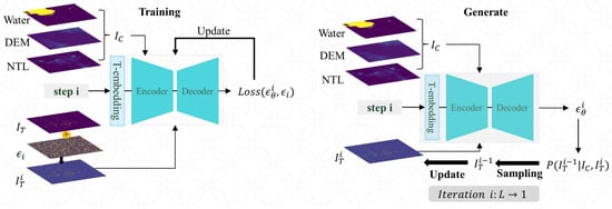
Figure 1.
Framework of the urban morphology prediction method based on the conditional diffusion model. During the training stage, the optimization objective of the conditional diffusion model is to minimize the distance between the predicted noise and the added noise. During the generation stage, the conditional diffusion model iteratively predicts noise and parameterizes the corresponding conditional distribution. The generation target is updated by sampling from this distribution until the end of the iterations, to obtain the final generated target.
- (1)
- Training stage. Specifically, multi-level Gaussian noise is added to the original to obtain the perturbed , after which and the guidance condition are used as inputs to the conditional diffusion model. The gradient of the conditional distribution is approximated with the noise predicted by the conditional diffusion model, where is the output of the conditional diffusion model.
- (2)
- Generation stage. The conditional distribution is parameterized with the noise predicted by the conditional diffusion model, and the generation target is updated by sampling from the distribution, until iteration is completed. Specifically, the pure noise is first sampled from the Gaussian distribution as the initial value of the generation target, which is used as input to the conditional diffusion model, along with the guidance condition . The conditional distribution is parameterized with the noise predicted by the conditional diffusion model, and the updated generation target is sampled from the distribution. The above process is iterated until the final generation target is sampled from the conditional distribution .
3.2.1. Training Stage
The attribute-based urban morphology prediction is modeled as a conditional distribution . For construction of the guidance condition , two methods are adopted in this paper for the experiments. The first method is to stack the images representing spatial and social attributes according to the channel to obtain (i.e., fusion1). The second method is to add the images representing spatial and social attributes element by element to obtain (i.e., fusion2).
The conditional diffusion model includes two stages: forward diffusion with added noise and backward diffusion with predicted noise. In the forward diffusion stage, isotropic Gaussian noise is added to the original generation target . The perturbed generation target follows a Gaussian distribution, as shown in Formulas (1) and (2), where is a parameter that obeys the linear growth strategy and I denotes the variance of the standard Gaussian distribution. By continuously adding isotropic Gaussian noise, the original generation target is gradually transformed into Gaussian noise. Therefore, the original target distribution is transformed into a standard Gaussian distribution. Forward diffusion does not involve training or updating the parameters of the conditional diffusion model.
In contrast, for backward diffusion, the perturbed generation target and the guidance condition are used as inputs to the conditional diffusion model , which is trained to predict the noise added by forward diffusion. The optimization objective of backward diffusion is to minimize the distance between the noise predicted by the conditional diffusion model and the noise added by forward diffusion. During the optimization process, multiple different levels of Gaussian noise are used for joint training. The optimization objectives for a single noise level and the overall levels are shown in Formulas (3) and (4).
Thus, the gradient of the conditional distribution can essentially be estimated under different noise levels.
3.2.2. Generation Stage
The function of the noise predicted by the conditional diffusion model is to estimate the gradient of the conditional distribution corresponding to different noise levels, thereby being able to parameterize the conditional Gaussian distribution of the backward diffusion, as shown in Formula (5), where represents the output of the conditional diffusion model and I denotes the variance of the standard Gaussian distribution.
To predict urban morphology, gradient-based sampling is needed, to generate an urban morphology map that matches the conditional distribution . According to the sampling strategy in ref. [13], a gradient-based annealing sampling method is used in this paper. The pseudo-code for the gradient-based annealing sampling method can be found in Algorithm 1.
| Algorithm 1 Gradient-Based Annealing Sampling Method |
|
Specifically, the pure noise is first sampled from the Gaussian distribution as the initial value of the generation target, which is used as input to the conditional diffusion model along with the guidance condition . The conditional diffusion model is used to predict the corresponding noise. The conditional distribution is then parameterized based on the predicted noise, and the generation target with a lower noise level is sampled from . The above process is repeated for L iterations to update the initial value of the generation target. The process of sampling from the conditional distribution is shown in Formula (6), where .
In addition, to prevent the degradation caused by ignoring the guidance condition when predicting noise using the condition diffusion model, the sampling strategy in ref. [40] is utilized. The noise that is used to parameterize the conditional distribution is represented as a linear combination of the output of the conditional diffusion model and the unconditional diffusion model , as shown in Formula (7). The parameter w is used to control the degree of guidance. By adjusting the parameter w, different biases can be achieved between the diversity and the correlation of the generation target.
4. Experiment and Discussion
4.1. Description of the Dataset
In this paper, the training and testing datasets published in ref. [10] were used to train and test the model. The training dataset contained four types of images, namely, urban built-up area images (as label), as well as corresponding NTL images, DEM images, and water area images, for a total of 9697 images of each type. The test dataset also included the above four types of images, with a total of 200 images for each type. The size of the images was 128 × 128, and each image represented a geographic unit of 100 km × 100 km, with each pixel representing approximately 780 m × 780 m. Detailed information on the sampling time and sampling location of the dataset can be found in ref. [10]. The urban built-up area image was a binary image, with 1 representing a built-up area and 0 representing a non-built-up area. Each pixel in the DEM image is the average elevation of the corresponding area, and the pixel value is scaled to 0-1. Each pixel in the NTL image is also an average measure of the corresponding area, and the pixel value is scaled to 0-1. The water area image is a binary image, with 0 representing the land area and 1 representing the water area. Figure 2 shows these four types of images.

Figure 2.
Visualization of the dataset sample. The urban built-up area images and the water area images are binary images with pixel values of 0 and 1, respectively. Each pixel in the DEM and NTL images represents the average value of the corresponding geographic area, and the pixel value is scaled to 0-1.
There are significant differences in samples from different urban areas, which can be intuitively reflected in the proportion and concentration of built-up areas. In this paper, a histogram of the number of samples with different proportions of built-up areas (i.e., first feature) was presented in the dataset, as shown in Figure 3. In addition, the variance in the centroid distance of the built-up areas (i.e., second feature) was calculated for each sample, and it was normalized accordingly, which could reflect the degree of concentration of urban development. A histogram of the number of urban samples representing different variances in the centroid distance in the built-up area of the dataset is shown in Figure 4.
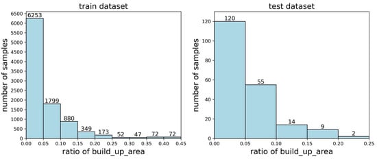
Figure 3.
Histograms of the dataset regarding the first feature. The left figure represents the results for the training dataset, and the right figure represents the results for the testing dataset.
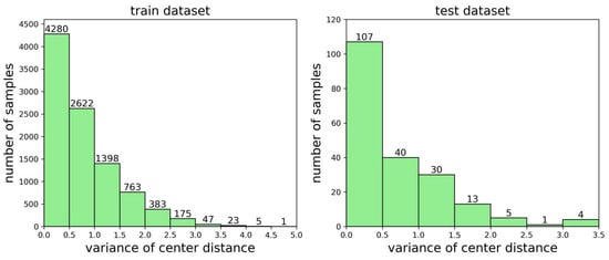
Figure 4.
Histograms of the dataset regarding the second feature. The left figure represents the results for the training dataset, and the right figure represents the results for the testing dataset.
Figure 3 and Figure 4 show that the distributions of the two types of statistical features in the training and testing datasets were similar. However, there was a significant difference in the extreme values of the two types of statistical features in the training and testing datasets, as shown in Table 1.

Table 1.
The extreme values of the two types of statistical features in the dataset.
4.2. Baseline Methods
In this paper, XGBoost, U-Net, CityGAN, and MetroGAN were used as baseline methods. The baseline methods were quantitatively compared with the method proposed in this paper from the perspective of multilevel metrics.
XGBoost is widely used as a classification model in urban geography research [41]. In this paper, NTL images, DEM images, and water area images were used as inputs to the model, and the model classified each pixel as a built-up or non-built-up area to obtain the prediction result.
U-Net is a widely used deep neural network model for image transformation tasks [42] and can predict a corresponding target image based on the input image. In this paper, NTL images, DEM images, and water area images were used as inputs to predict the corresponding urban built-up area image.
CityGAN is an early model used to predict urban morphology. In this paper, NTL images, DEM images, and water area images were used as conditions to train this model to output the corresponding urban morphology.
MetroGAN is a recent model used for urban morphology prediction, and it has achieved the best results. This model uses NTL images, DEM images, and water area images as conditions to train and output the corresponding urban morphology. Moreover, this model introduces geographical constraint loss and uses a progressive generation strategy to achieve high-quality prediction results.
4.3. Experiment and Parameter Setup
The focus of this paper is predicting attribute-based urban morphology, where multi-source attributes are aggregated as a guidance condition. However, different methods of aggregating multi-source attributes have different impacts on the generation target. Therefore, for the aggregation method of the guidance condition, two experiments were conducted in this paper. The first aggregation method (i.e., fusion1) stacked the images representing multi-source attributes by channel. The calculation process is shown in Formula (8). The second aggregation method was to add the images representing multi-source attributes element-wise. The calculation process is shown in Formula (9).
For the parameters in the experiment, the noise level in forward diffusion was set to 1000 steps . The noise variance () was linear growth, where the initial value was set to 0.0001 and the final value was set to 0.02. This setting followed that of the DDPM model [13]. The training epochs were set to 500, and the optimizer was set to Adam. The initial learning rate was set to 1 × 10⁻⁴, while a cosine learning rate decay strategy was used. The batch size of the training stage was set to 64. The computing device used in the experiment was an NVIDIA A6000 GPU with the operating system Ubuntu 22.04. In the generation stage, a threshold of 0.9 was used to perform numerical cropping on the final generation target. Pixels larger than the threshold were mapped to 1, and pixels smaller than the threshold were mapped to 0.
4.4. Evaluations
Based on the evaluation framework proposed in ref. [10], the generation target was quantitatively evaluated and verified in this paper. This included the following two aspects:
- (1)
- Evaluating whether the generation target was similar to the actual label in terms of the visual features.
- (2)
- Verifying whether the spatial morphology of the generation target was consistent with the actual label.
For the evaluation of visual features, the generation target was compared with the actual label at three levels: low-level pixel features, shallow structural features, and deep structural features. Since urban areas follow fractal structural laws at the macro level, fractal dimensions were used to validate the consistency of the generation targets with the actual labels. Table 2 summarizes the evaluation and validation metrics.

Table 2.
Summary of the evaluation and validation metrics.
4.4.1. Low-Level Pixel Feature
For low-level pixel features, the peak signal-to-noise ratio () was used as the metric, which was calculated using Formulas (10) and (11). H and W denote the height and width of the image, and denote the pixel values at the same position for the two images to be compared, and denotes the maximum possible pixel value in the image. The larger the PSNR, the greater the similarity between the generation target and the actual label in terms of the low-level pixel features.
4.4.2. Shallow Structural Feature
For the shallow structural features, the [43] was used as the metric. The can comprehensively compare two images in terms of the brightness, contrast, and shallow visual structure. The larger the , the smaller the differences in the brightness, contrast, and shallow image structure between two images. The calculation method is shown in Formula (12). The and denote the means of the pixels in the two images, and denote the variances in the pixels in the two images, and denotes the covariance of the pixels in the two images. and are constants used to stop the denominator being zero in the division.
4.4.3. Deep Structural Feature
For deep structural features, LPIPS [44] was used as the metric. LPIPS uses deep convolutional neural networks to measure the multi-level global similarity of two images, and the measurement result is well matched with human cognition of the images. The smaller the LPIPS, the greater the global similarity between two images. The calculation method is shown in Formula (13). L denotes the feature extraction network containing L layers, and denote the height and width of the feature map in the layer, denotes the scaling factor for all C channels of the feature map in layer, and and denote the pixel values at the same position of the feature map of the two images.
4.4.4. Spatial Morphology Feature
The fractal dimension is an important indicator of the spatial morphology of an urban area. Based on ref. [45], the box counting method was used to calculate the fractal dimension (FD) of the generated target, as shown in Formula (14). r denotes the side length of the box, and denotes the number of boxes needed to cover the image.
4.5. Experimental Results
4.5.1. Evaluation of the Multi-Level Visual Features
In this paper, the generation targets were evaluated using three levels of visual features—low-level pixel features, shallow structural features, and deep structural feature—and were compared with four baseline methods, as shown in Table 3 (the results of the baseline methods are from ref. [10]). The parameter w used in the sampling process was fixed at 0.1.

Table 3.
Evaluation results in terms of visual features.
The PSNR metric was improved by 5.5% (fusion1) and 6.0% (fusion2) compared to the best baseline method and the XGBoost model was significantly lower than the other methods. The SSIM metric was improved by 5.9% (fusion1) and 5.6% (fusion2) compared to the best baseline method. The LPIPS metric was improved by 13.2% (fusion1) and 7.1% (fusion2) compared to the best baseline method, and the XGBoost model was significantly higher than the other methods. These results suggest that constructing a guidance condition by summing images representing multi-source attributes element by element allows a conditional diffusion model to learn low-level pixel feature more accurately. However, constructing a guidance condition by stacking images representing multiple source attributes by channel allows the conditional diffusion model to learn shallow and deep structural features more accurately. In addition, the results in Table 3 show that there was a significant gap between the XGBoost model and other models in terms of the PSNR metric and LPIPS metric.
The results in Table 3 show that this paper achieved an enhancement in all evaluation metrics. In terms of low-level pixel features and shallow structural features, this paper realized a more than 5.5% improvement compared with the best baseline method, which indicates that the method proposed in this paper can better capture the low-level features of urban systems. In addition to the low-level pixel features and shallow structural features, the high-level global structural features could more comprehensively reflect the spatial pattern similarity between the prediction results and the real labels. In terms of the LPIPS metric, this paper achieved a 13.2% improvement compared to the best baseline method, which indicates that the method proposed in this paper could better capture the deep structure of urban systems.
The learning objective of CityGAN and MetroGAN models is the distribution of urban morphology. However, the diversity and complexity of urban systems make it difficult to directly approximate this distribution. In this paper, we changed the learning objective to implicitly approximate the gradient of the distribution by predicting noise through a diffusion model, which reduced the learning difficulty. As a result, using the same data for training, the method proposed in this paper could more accurately approximate the gradient of the urban form distribution, and thus indirectly and accurately approximate the urban morphology distribution. In addition, the CityGAN and MetroGAN models obtain generation targets through one-step sampling, while the method proposed in this paper obtains generated targets through successive multi-step sampling operations, which further ensures the accuracy of the generated targets.
Figure 5 shows some generation targets (as Generate) and corresponding labels, where the parameter w of the sampling process was fixed to 0.1. Each row of the left figure and right figure represents a different urban area. The first three columns are NTL images, DEM images, and water area images of urban areas. The fourth column is the real built-up area images of the urban areas. The fifth column of the left figure is the prediction results obtained based on the first aggregation method. The fifth column of the right figure is the prediction results based on the second aggregation method. The closer the images in the fourth column are to the images in the fifth column, the more accurate the predictions in this paper.
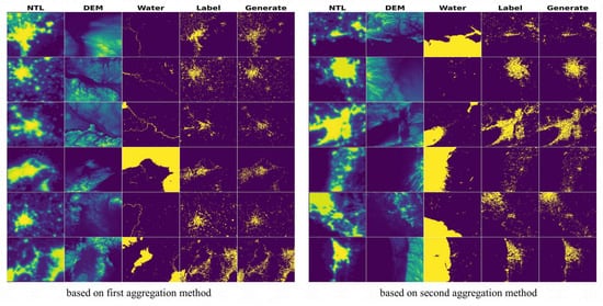
Figure 5.
Some generation targets. The color bar is consistent with Figure 2. The left figure shows the generation targets obtained by constructing a guidance condition based on the first aggregation method. The right figure shows the generation targets obtained by constructing a guidance condition based on the second aggregation method.
4.5.2. Validation of the Spatial Morphology Feature
To verify whether the spatial morphological features of the generation targets (as Generate) were similar to the corresponding labels, the fractal dimension was used for verification. The fractal dimensions of each generation target (the parameter w of the sampling process was fixed to 0.1) and the corresponding label were calculated separately. Then, the Pearson correlation coefficient of the two fractal dimensions was calculated, as shown in Figure 6. The Pearson correlation coefficient for the first aggregation method of the guidance condition was 0.760. The Pearson correlation coefficient for the second aggregation method of the guidance condition was 0.647. This suggests that constructing a guidance condition by stacking images representing multiple attributes by channels allowed the conditional diffusion model to learn spatial morphological feature more accurately.
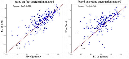
Figure 6.
Fractal dimension - statistics of the generation targets and corresponding labels.
The differences between the fractal dimensions of the generation targets and the fractal dimensions of the corresponding labels were calculated. The five segments 0–0.1, 0.1–0.2, 0.2–0.3, 0.3–0.4, and >0.4 were divided at intervals of 0.1. Within each segment, the number of samples, the average fractal dimension of the generation targets, the average fractal dimension of the labels, and the average proportion of built-up areas of the labels were counted separately. The statistical results are shown in Table 4 and Table 5.

Table 4.
Statistical results for the first aggregation method.

Table 5.
Statistical results for the second aggregation method.
As shown in Table 4, there were 177 samples with a fractal dimension difference of less than 0.2 and 7 samples with a difference of more than 0.3. As shown in Table 5, there were 159 samples with a fractal dimension difference of less than 0.2 and 19 samples with a difference of more than 0.3. This shows that stacking images representing attributes by channel to construct a guidance condition enabled the conditional diffusion model to learn spatial morphological feature more accurately.
Figure 7 and Figure 8 show some bad samples of generation targets that were significantly different from the corresponding labels. As shown in Figure 7, the fractal dimensions of the bad samples that were generated via the first aggregation method were significantly lower than those of the corresponding labels. As shown in Figure 8, the fractal dimension of the bad samples that were generated via the second aggregation method had the opposite trend to those of the corresponding labels, which were relatively small when the fractal dimension of the labels was relatively large, and vice versa.

Figure 7.
Bad samples based on the first aggregation method.
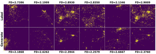
Figure 8.
Bad samples based on the second aggregation method.
4.6. Ablation Experiments
For the two types of aggregation methods for the guidance condition and the parameter w used in the generation stage, ablation experiments were conducted to investigate their effect on the generation target. The parameter w was set to ten different values ranging from 0.0 to 4.0, which could reflect the effects of smaller and larger correlations of the guidance condition on the generation targets. Table 6 shows the results of the ablation experiment based on the first aggregation method with different values of parameter w. Table 7 shows the results of the ablation experiment based on the second aggregation method with different values of the parameter w. Figure 9 and Figure 10 show some generation targets based on the two types of aggregation methods with different values of parameter w and the corresponding labels.

Table 6.
Results based on different values of the parameter w with the first aggregation method.

Table 7.
Results based on different values of the parameter w with the second aggregation method.
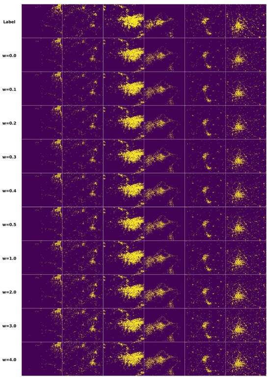
Figure 9.
Generation targets based on different values of the parameter w under the first aggregation method. The first column shows the corresponding labels.
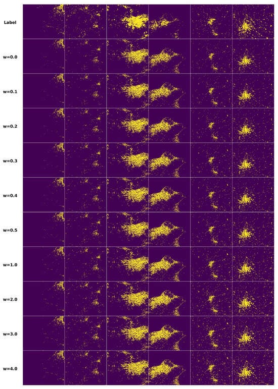
Figure 10.
Generation targets based on different values of the parameter w under the second aggregation method. The first column shows the corresponding labels.
4.6.1. Comparison of Two Types of Aggregation Method
The use of the same parameter w allowed a fair comparison of two types of aggregation methods on the generation targets. By comparing Table 6 and Table 7, it can be seen that the targets generated based on the first aggregation method were always better for the three metrics of SSIM, LPIPS, and spatial morphological features. Therefore, stacking images representing multi-source attributes by channel enabled the conditional diffusion models to better utilize multi-source attributes to predict urban morphology.
In addition, the confusion matrix was calculated by counting all the images in the testing dataset with the corresponding predictions, as shown in Figure 11. The elements of each position in the confusion matrix represent the number and proportion of pixels. From the confusion matrix, it can be seen that the prediction accuracy of the first aggregation method for built-up areas was 36.17%, which was higher than that of the second method, which was 33.91%; while the prediction accuracy of the second aggregation method for non-built-up areas was 97.76%, which was slightly higher than that of the first method, which was 97.56%. This indicates that the first aggregation method was more advantageous.
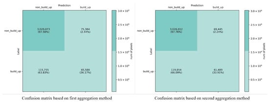
Figure 11.
Confusion matrix for the prediction results of the two types of fusion method.
4.6.2. Comparison of Different Parameters w
As shown in Table 6 and Table 7, under the two types of aggregation method, both the PSNR metric and SSIM metric decreased significantly with increasing w, which indicates that the difference between the generation targets and the corresponding labels in terms of low-level pixel feature and shallow structural feature gradually increased. The LPIPS metric first decreased and then increased, which indicated that the difference between the generation targets and the corresponding labels in terms of deep structural feature first decreased and then increased. For the spatial morphology feature, the correlation between the fractal dimension of the generation targets and the fractal dimension of the corresponding labels decreased significantly after the parameter was w increased to a certain value, which indicates that the correlation between the generation target and the multi-source attributes was significantly weaker after the parameter w exceeded a certain value.
4.7. Discussion
Due to the complexity and diversity of urban morphology, it is unrealistic to assume that they obey a certain probability distribution that can be directly approximated. Distinct from models that directly approximate the urban morphology distribution, diffusion models implicitly learn the gradient of an urban morphology distribution by predicting the noise and thus indirectly approximate the urban morphology distribution. In general, for complex target distributions, the form of the gradient is usually simpler. Thus, a diffusion model has a clear advantage when trained using the same dataset. In this paper, attribute-based urban morphology prediction was modeled as a conditional distribution. The gradient of the conditional distribution was estimated by predicting the noise through a conditional diffusion model, and a gradient-based annealing sampling method was used to generate an urban morphology map matching the approximated conditional distribution. Compared to one-step sampling, this paper used consecutive multi-step sampling in the generation phase, which improved the generation quality through decomposition. The experimental results showed that compared with baseline methods, the urban morphology prediction method proposed in this paper achieved enhancements in all evaluation metrics.
For the construction of a guidance condition, experiments with two types of method, stacking by channel and summing element-by-element, were conducted. The ablation experiments showed that the aggregation method of stacking images representing multi-source attributes by channel retained the attribute information more completely, which enabled the conditional diffusion model to estimate gradients more accurately and facilitated the prediction of urban morphology.
Traditional prediction methods are mainly based on statistical spatio-temporal interaction information. This information is acquired with a lag and cannot fully utilize the large number of existing remote sensing images. Aiming at the above problems, the method proposed in this paper has obvious advantages. First, remote sensing images are easy to obtain and have high timeliness. Second, by inputting the time series images, the method proposed in this paper can predict the urban morphology in the corresponding time series, which helps researchers to explore urban renewal in the time series.
5. Conclusions and Future Work
Inspired by score-based models, an urban morphology prediction method based on a conditional diffusion model was proposed in this paper. First, attribute-based urban morphology prediction was modeled as a conditional distribution. Second, the gradient of the conditional distribution was estimated by predicting noise through a conditional diffusion model, and the conditional distribution was then implicitly approximated based on the gradient. In the generation stage, the corresponding conditional distribution was parameterized based on the noise predicted by the conditional diffusion model, and the generation target was obtained via a gradient-based annealing sampling method. Compared with the best baseline method, the proposed method achieved 5.5% and 5.9% improvements for the low-level pixel feature and shallow structural feature, respectively, and a 13.2% significant improvement in the deep structural feature. The experimental results verified the effectiveness of the strategy of using the conditional diffusion model to estimate the gradient and thus implicitly approximate the urban morphology distribution. The ablation experiments showed that the construction method of stacking images representing multi-source attributes by channel retained more complete attribute information, which allowed the conditional diffusion model to estimate gradients more accurately. In future work, more attributes will be used to predict urban morphology. In addition, based on the gradient of the distribution estimated by the conditional diffusion model, the gradient could be used to measure the impact of different attributes on predicting urban morphology.
Author Contributions
Conceptualization, T.S. and H.L.; methodology, T.S. and H.L.; software, T.S.; validation, T.S., F.L., M.Z. and M.L.; formal analysis, T.S. and C.P.; investigation, T.S., M.Z. and L.Z.; resources, T.S.; data curation, T.S.; writing—original draft preparation, T.S., H.L., F.L., M.Z., M.L., C.P. and L.Z.; writing—review and editing, T.S., C.P., H.L. and L.Z.; visualization, T.S.; supervision, H.L.; project administration, H.L.; funding acquisition, H.L. and L.Z. All authors have read and agreed to the published version of the manuscript.
Funding
This work was supported by the National Natural Science Foundation of China [grant numbers 42171458.
Data Availability Statement
The datasets that support the findings of this study are openly available at https://github.com/zwy-Giser/MetroGAN, accessed on 6 September 2023.
Conflicts of Interest
The authors declare that they have no known competing financial interests or personal relationships that could have appeared to influence the work reported in this paper.
References
- Næss, P. Built environment, causality and urban planning. Plan. Theory Pract. 2016, 17, 52–71. [Google Scholar] [CrossRef]
- Bettencourt, L.M.; Lobo, J.; Helbing, D.; Kühnert, C.; West, G.B. Growth, innovation, scaling, and the pace of life in cities. Proc. Natl. Acad. Sci. USA 2007, 104, 7301–7306. [Google Scholar] [CrossRef] [PubMed]
- Batty, M. The size, scale, and shape of cities. Science 2008, 319, 769–771. [Google Scholar] [CrossRef] [PubMed]
- Mo, Y.; Guo, Z.; Zhong, R.; Song, W.; Cao, S. Urban Functional Zone Classification Using Light-Detection-and-Ranging Point Clouds, Aerial Images, and Point-of-Interest Data. Remote Sens. 2024, 16, 386. [Google Scholar] [CrossRef]
- Li, R.; Dong, L.; Zhang, J.; Wang, X.; Wang, W.X.; Di, Z.; Stanley, H.E. Simple spatial scaling rules behind complex cities. Nat. Commun. 2017, 8, 1841. [Google Scholar] [CrossRef]
- Fuglsang, M.; Münier, B.; Hansen, H.S. Modelling land-use effects of future urbanization using cellular automata: An Eastern Danish case. Environ. Model. Softw. 2013, 50, 1–11. [Google Scholar] [CrossRef]
- Zhao, W.; Li, M.; Wu, C.; Zhou, W.; Chu, G. Identifying urban functional regions from high-resolution satellite images using a context-aware segmentation network. Remote Sens. 2022, 14, 3996. [Google Scholar] [CrossRef]
- Goodfellow, I.; Pouget-Abadie, J.; Mirza, M.; Xu, B.; Warde-Farley, D.; Ozair, S.; Courville, A.; Bengio, Y. Generative adversarial nets. Adv. Neural Inf. Process. Syst. 2014, 27. [Google Scholar] [CrossRef]
- Karras, T.; Laine, S.; Aila, T. A style-based generator architecture for generative adversarial networks. In Proceedings of the IEEE/CVF Conference on Computer Vision and Pattern Recognition, Long Beach, CA, USA, 15–20 June 2019; pp. 4401–4410. [Google Scholar]
- Zhang, W.; Ma, Y.; Zhu, D.; Dong, L.; Liu, Y. Metrogan: Simulating urban morphology with generative adversarial network. In Proceedings of the 28th ACM SIGKDD Conference on Knowledge Discovery and Data Mining, Washington, DC, USA, 14–18 August 2022; pp. 2482–2492. [Google Scholar]
- Albert, A.; Kaur, J.; Strano, E.; Gonzalez, M. Spatial sensitivity analysis for urban land use prediction with physics-constrained conditional generative adversarial networks. arXiv 2019, arXiv:1907.09543. [Google Scholar]
- Albert, A.; Kaur, J.; Gonzalez, M.C. Using convolutional networks and satellite imagery to identify patterns in urban environments at a large scale. In Proceedings of the 23rd ACM SIGKDD International Conference on Knowledge Discovery and Data Mining, Halifax, NS, Canada, 13–17 August 2017; pp. 1357–1366. [Google Scholar]
- Ho, J.; Jain, A.; Abbeel, P. Denoising diffusion probabilistic models. Adv. Neural Inf. Process. Syst. 2020, 33, 6840–6851. [Google Scholar]
- Dhariwal, P.; Nichol, A. Diffusion models beat gans on image synthesis. Adv. Neural Inf. Process. Syst. 2021, 34, 8780–8794. [Google Scholar]
- Liu, X.; Park, D.H.; Azadi, S.; Zhang, G.; Chopikyan, A.; Hu, Y.; Shi, H.; Rohrbach, A.; Darrell, T. More control for free! image synthesis with semantic diffusion guidance. In Proceedings of the IEEE/CVF Winter Conference on Applications of Computer Vision, Waikoloa, HI, USA, 3–7 January 2023; pp. 289–299. [Google Scholar]
- Efron, B. Tweedie’s formula and selection bias. J. Am. Stat. Assoc. 2011, 106, 1602–1614. [Google Scholar] [CrossRef] [PubMed]
- Luo, C. Understanding diffusion models: A unified perspective. arXiv 2022, arXiv:2208.11970. [Google Scholar]
- Li, X.; Gong, P. Urban growth models: Progress and perspective. Sci. Bull. 2016, 61, 1637–1650. [Google Scholar] [CrossRef]
- Iacono, M.; Levinson, D.; El-Geneidy, A. Models of transportation and land use change: A guide to the territory. J. Plan. Lit. 2008, 22, 323–340. [Google Scholar] [CrossRef]
- Hunt, J.D.; Kriger, D.S.; Miller, E.J. Current operational urban land-use–transport modelling frameworks: A review. Transp. Rev. 2005, 25, 329–376. [Google Scholar] [CrossRef]
- Liu, X.; Ma, L.; Li, X.; Ai, B.; Li, S.; He, Z. Simulating urban growth by integrating landscape expansion index (LEI) and cellular automata. Int. J. Geogr. Inf. Sci. 2014, 28, 148–163. [Google Scholar] [CrossRef]
- Ozturk, D. Urban growth simulation of Atakum (Samsun, Turkey) using cellular automata-Markov chain and multi-layer perceptron-Markov chain models. Remote Sens. 2015, 7, 5918–5950. [Google Scholar] [CrossRef]
- Matthews, R.B.; Gilbert, N.G.; Roach, A.; Polhill, J.G.; Gotts, N.M. Agent-based land-use models: A review of applications. Landsc. Ecol. 2007, 22, 1447–1459. [Google Scholar] [CrossRef]
- Irwin, E.G.; Geoghegan, J. Theory, data, methods: Developing spatially explicit economic models of land use change. Agric. Ecosyst. Environ. 2001, 85, 7–24. [Google Scholar] [CrossRef]
- Santé, I.; García, A.M.; Miranda, D.; Crecente, R. Cellular automata models for the simulation of real-world urban processes: A review and analysis. Landsc. Urban Plan. 2010, 96, 108–122. [Google Scholar] [CrossRef]
- Li, X.; Liu, X.; Yu, L. A systematic sensitivity analysis of constrained cellular automata model for urban growth simulation based on different transition rules. Int. J. Geogr. Inf. Sci. 2014, 28, 1317–1335. [Google Scholar] [CrossRef]
- Shu, B.; Bakker, M.M.; Zhang, H.; Li, Y.; Qin, W.; Carsjens, G.J. Modeling urban expansion by using variable weights logistic cellular automata: A case study of Nanjing, China. Int. J. Geogr. Inf. Sci. 2017, 31, 1314–1333. [Google Scholar] [CrossRef]
- Wu, F. Calibration of stochastic cellular automata: The application to rural-urban land conversions. Int. J. Geogr. Inf. Sci. 2002, 16, 795–818. [Google Scholar] [CrossRef]
- Tian, G.; Ouyang, Y.; Quan, Q.; Wu, J. Simulating spatiotemporal dynamics of urbanization with multi-agent systems—A case study of the Phoenix metropolitan region, USA. Ecol. Model. 2011, 222, 1129–1138. [Google Scholar] [CrossRef]
- Crooks, A.; Castle, C.; Batty, M. Key challenges in agent-based modelling for geo-spatial simulation. Comput. Environ. Urban Syst. 2008, 32, 417–430. [Google Scholar] [CrossRef]
- Parker, D.C.; Manson, S.M.; Janssen, M.A.; Hoffmann, M.J.; Deadman, P. Multi-agent systems for the simulation of land-use and land-cover change: A review. Ann. Assoc. Am. Geogr. 2003, 93, 314–337. [Google Scholar] [CrossRef]
- Albert, A.; Strano, E.; Kaur, J.; González, M. Modeling urbanization patterns with generative adversarial networks. In Proceedings of the IGARSS 2018–2018 IEEE International Geoscience and Remote Sensing Symposium, Valencia, Spain, 22–27 July 2018; pp. 2095–2098. [Google Scholar]
- Sun, S.; Mu, L.; Feng, R.; Wang, L.; He, J. GAN-based LUCC prediction via the combination of prior city planning information and land-use probability. IEEE J. Sel. Top. Appl. Earth Obs. Remote Sens. 2021, 14, 10189–10198. [Google Scholar] [CrossRef]
- Huang, C.; Zhang, G.; Yao, J.; Wang, X.; Calautit, J.K.; Zhao, C.; An, N.; Peng, X. Accelerated environmental performance-driven urban design with generative adversarial network. Build. Environ. 2022, 224, 109575. [Google Scholar] [CrossRef]
- Ibrahim, H.; Khattab, Z.; Khattab, T.; Abraham, R. Generative Adversarial Network Approach to Future Sermonizing of Housing Dispersal in Emerging Cities. J. Urban Plan. Dev. 2022, 148, 04021067. [Google Scholar] [CrossRef]
- Zhang, Y.; Li, Y.; Zhou, X.; Kong, X.; Luo, J. Curb-gan: Conditional urban traffic estimation through spatio-temporal generative adversarial networks. In Proceedings of the 26th ACM SIGKDD International Conference on Knowledge Discovery & Data Mining, Virtual Event, 23–27 August 2020; pp. 842–852. [Google Scholar]
- He, S.; Luo, Q.; Du, R.; Zhao, L.; He, G.; Fu, H.; Li, H. STGC-GNNs: A GNN-based traffic prediction framework with a spatial–temporal Granger causality graph. Phys. Stat. Mech. Its Appl. 2023, 623, 128913. [Google Scholar] [CrossRef]
- Luo, Q.; He, S.; Han, X.; Wang, Y.; Li, H. LSTTN: A Long-Short Term Transformer-based spatiotemporal neural network for traffic flow forecasting. Knowl.-Based Syst. 2024, 293, 111637. [Google Scholar] [CrossRef]
- Zhu, J.; Han, X.; Deng, H.; Tao, C.; Zhao, L.; Wang, P.; Lin, T.; Li, H. KST-GCN: A knowledge-driven spatial-temporal graph convolutional network for traffic forecasting. IEEE Trans. Intell. Transp. Syst. 2022, 23, 15055–15065. [Google Scholar] [CrossRef]
- Ho, J.; Salimans, T. Classifier-free diffusion guidance. arXiv 2022, arXiv:2207.12598. [Google Scholar]
- Shao, Z.; Ahmad, M.N.; Javed, A. Comparison of Random Forest and XGBoost Classifiers Using Integrated Optical and SAR Features for Mapping Urban Impervious Surface. Remote Sens. 2024, 16, 665. [Google Scholar] [CrossRef]
- Ronneberger, O.; Fischer, P.; Brox, T. U-net: Convolutional networks for biomedical image segmentation. In Proceedings of the Medical Image Computing and Computer-Assisted Intervention–MICCAI 2015: 18th International Conference, Munich, Germany, 5–9 October 2015; Springer: Berlin/Heidelberg, Germany, 2015; pp. 234–241. [Google Scholar]
- Wang, Z.; Bovik, A.C.; Sheikh, H.R.; Simoncelli, E.P. Image quality assessment: From error visibility to structural similarity. IEEE Trans. Image Process. 2004, 13, 600–612. [Google Scholar] [CrossRef]
- Zhang, R.; Isola, P.; Efros, A.A.; Shechtman, E.; Wang, O. The unreasonable effectiveness of deep features as a perceptual metric. In Proceedings of the IEEE Conference on Computer Vision and Pattern Recognition, Salt Lake City, UT, USA, 18–23 June 2018; pp. 586–595. [Google Scholar]
- Sarkar, N.; Chaudhuri, B.B. An efficient differential box-counting approach to compute fractal dimension of image. IEEE Trans. Syst. Man Cybern. 1994, 24, 115–120. [Google Scholar] [CrossRef]
Disclaimer/Publisher’s Note: The statements, opinions and data contained in all publications are solely those of the individual author(s) and contributor(s) and not of MDPI and/or the editor(s). MDPI and/or the editor(s) disclaim responsibility for any injury to people or property resulting from any ideas, methods, instructions or products referred to in the content. |
© 2024 by the authors. Licensee MDPI, Basel, Switzerland. This article is an open access article distributed under the terms and conditions of the Creative Commons Attribution (CC BY) license (https://creativecommons.org/licenses/by/4.0/).