Abstract
In response to the growing demand for railway obstacle monitoring, lidar technology has emerged as an up-and-coming solution. In this study, we developed a mechanical 3D lidar system and meticulously calibrated the point cloud transformation to monitor specific areas precisely. Based on this foundation, we have devised a novel set of algorithms for obstacle detection within point clouds. These algorithms encompass three key steps: (a) the segmentation of ground point clouds and extraction of track point clouds using our RS-Lo-RANSAC (region select Lo-RANSAC) algorithm; (b) the registration of the BP (background point cloud) and FP (foreground point cloud) via an improved Robust ICP algorithm; and (c) obstacle recognition based on the VFOR (voxel-based feature obstacle recognition) algorithm from the fused point clouds. This set of algorithms has demonstrated robustness and operational efficiency in our experiments on a dataset obtained from an experimental field. Notably, it enables monitoring obstacles with dimensions of 15 cm × 15 cm × 15 cm. Overall, our study showcases the immense potential of lidar technology in railway obstacle monitoring, presenting a promising solution to enhance safety in this field.
1. Introduction
Railway safety is a topic of great concern to people, and in recent years, train accidents caused by obstacles have occurred frequently [1]. Due to the complexity of railway terrain, the intrusion of blocks has features such as randomness, suddenness, and unpredictability [2]. Therefore, the real-time monitoring of obstacles has become an urgent demand [3].
Most research on railway obstacle intrusion focuses on visual detection [4]. However, current optical systems face several challenges, including susceptibility to lighting conditions; reduced obstacle recognition in harsh environments such as rain, snow, and fog; and difficulty in accurately identifying the distance information of obstacles [5]. Staniša et al. [6] proposed a machine learning-based strategy for obstacle detection in cases of pixel-level differences to overcome the low-pixel resolution of the camera system under adverse environmental conditions. Meanwhile, Anand et al. [7] introduced a visual enhancement system that combines infrared cameras and other devices to improve its detection rate in adverse weather conditions. Lidar is an active sensor. It emits laser pulses towards an object and calculates the distance by collecting and analyzing the echo signals reflected from the object. In recent years, lidar sensors have been widely used in obstacle detection because they are immune to environmental light, have a quick response time, and effectively detect distant obstacles [8,9]. The mainstream 3D lidar used in obstacle measurement includes MEMS (Micro-electro Mechanical System) lidar and traditional mechanical lidar. Due to the faster scanning speed, MEMS lidar is used more for dynamic obstacle detection. Zheng et al. [10] combined 2D MEMS lidar with drones to calibrate coordinates on sparse point cloud maps. They utilized a clustering algorithm to detect obstacles in motion. MEMS lidar uses voltage to drive a two-axis MEMS mirror to realize scanning in a three-dimensional direction [11]. When we use it to detect railway obstacles, the scanning method, as shown in Figure 1a, is usually adopted to realize remote detection. However, this method will bring the scanning of blind areas. Traditional mechanical lidar uses a motor to carry the single-line lidar to realize three-dimensional scanning. It can achieve a denser distribution of scan lines by slowing down the motor speed, so the imaging detail is outstanding (Figure 1b). Vitor et al. [12] performed the output of 3D point clouds by combining 2D lidar and inertial measurement units along the railway. They completed the detection of railway obstacles in the small crossing area.
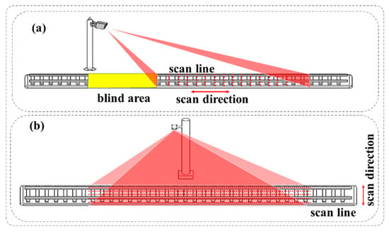
Figure 1.
(a) The scanning of the rail by MEMS lidar. (b) The scanning of the rail by 3D mechanical lidar.
Similarly, there has been extensive research on algorithms for point cloud obstacle detection [13,14]. Gao et al. [15] analyzed the geometric properties of obstacles based on non-uniform density point clouds and proposed an improved dynamic clustering algorithm that enhances the accuracy of traditional density-based clustering algorithms in autonomous driving. However, the algorithm’s stability decreases when dealing with parallel or distant obstacles. Before conducting segmented clustering to identify the barriers, Anand et al. [16] performed segmentation preprocessing on the ground point cloud. By dividing the ground point cloud into squares and conducting statistical analysis on the points within each square, they successfully achieved ground point cloud segmentation under different slopes. This algorithm demonstrates better environmental adaptability than traditional segmentation algorithms such as RANSAC and voxel-based algorithms for point cloud segmentation. Similarly, algorithms based on machine learning have been introduced into obstacle detection using lidar [17,18]. However, achieving a balance between timeliness and accuracy has been proven to be difficult for these algorithms. Currently, the application of lidar in obstacle detection is still focused on detecting large obstacles such as cars and pedestrians, and a small number of research studies have used it for detecting small obstacles [19]. Vitor et al. [12] used a 2D laser scanner to design an obstacle detection device for railway intersections, successfully completing the recognition of obstacles with a height of 30 cm. However, the operating distance of the device is limited to a range of 10 m. J. Li [20] proposed an obstacle detection algorithm to eliminate ground disturbances using a 3D lidar and a biaxial rotating platform, which enables the device to detect obstacles with a height of 10 cm. However, the operating range of the device is also greatly limited. Therefore, developing a lidar device and robust algorithm that can detect small obstacles within a certain range has become an urgent need.
Based on the above discussion, we have designed a regionally adjustable 3D lidar system that can be used for railway obstacle monitoring and developed a new obstacle-monitoring method based on the fusion of background and foreground point clouds. Our lidar system and obstacle recognition algorithm can avoid the repetitive labor of manual inspections and errors caused by subjective judgments. Meanwhile, the resolution of video surveillance in low-light conditions such as darkness and tunnels seriously affect the accuracy of obstacle detection. Our lidar system has the ability to solve this limitation.
We fully implemented everything from hardware selection to system implementation during the system design. We utilized a high-precision servo motor, a PLC (programmable logic controller), and a single-line lidar to create a 3D mechanical lidar with an adjustable scanning area (by adjusting the scanning speed and pitch angle range of the servo motor, we can obtain different scanning areas). Furthermore, we thoroughly discussed the calibration of coordinate errors for objects during the scanning process.
Then, we developed an obstacle detection algorithm suitable for large-scale ground point clouds and mainly discussed several key steps of the algorithm. We preprocessed the point cloud in the track area in the first stage using a statistical outlier filter. In the second stage, to improve the efficiency and robustness of ground point cloud segmentation, we proposed a region-select random sample consensus algorithm (RS-Lo-RANSAC) to segment the ground and extract the track model. In the following stage, we used an improved Robust ICP algorithm to perform registration on the background point cloud (fixed point cloud without obstacles in the track area) and foreground point cloud (real-time point clouds in the track area that may contain obstacles), achieving good consistency. Finally, we proposed an obstacle voxel-based feature obstacle recognition (VFOR) to achieve the stable detection of small obstacles in the railway region.
The contributions of this article are as follows:
- (a)
- We have developed a region-adjustable 3D mechanical lidar suitable for railway obstacle detection, achieving the entire process from hardware system selection to software implementation. We also performed accurate corrections on lidar point clouds.
- (b)
- We have developed a novel set of obstacle detection algorithms for lidar point clouds, which enables the high-precision monitoring of obstacles in the track area.
- (c)
- We have improved and experimented on the Lo-RANSAC and Robust ICP algorithms in the process, which has enhanced their robustness and operational efficiency, making them applicable in most cases.
This paper is organized as follows. In Section 2, the components of the system are introduced, including the coordinate transformation of point cloud information and precise error correction. Section 3 discusses the algorithm’s processes and various steps, while Section 4 presents the experimental results. Finally, the conclusion is summarized.
2. Overall System Structure
As shown in Figure 2a, the hardware components of the entire system include a 2D scanning lidar rangefinder, a high-precision servo motor, and a PLC. The design and implementation of the 2D lidar rangefinder are not within the scope of this article’s discussion, and it achieves scanning along the lateral line using fixed angular resolution. The servo motor carries the 2D lidar to realize the acquisition of 3D information.
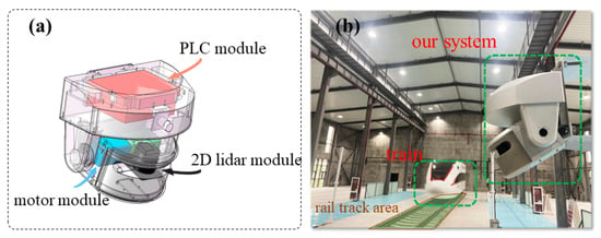
Figure 2.
(a) The main hardware components of our 3D lidar system. (b) The equipment is used in the experimental field and the site includes standard railway tracks.
A 2D lidar emits pulses at a fixed frequency to obtain the detected object’s distance R and lateral angle resolution. The PLC receives real-time elevation angle measurements. The scanning principle is shown in Figure 3a. The 2D lidar is designed to perform horizontal scans at a fixed frequency, providing pulse distance R for a fixed lateral angle resolution δ. Simultaneously, a high-precision specialized motor drives the 2D lidar for pitch scanning while under load, achieving precise real-time acquisition of pitch angles during operation. With this information, the conversion relationship of the three-dimensional Cartesian coordinate values of the detection point can be obtained (Figure 3b).
where represents the pulse’s pitch angle, represents the horizontal angle, R represents pulse distance, and H represents the height of the system.
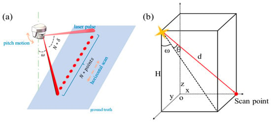
Figure 3.
(a) The scanning mechanism of 3D mechanical lidar. (b) Coordinate transformation relationship for point cloud.
Precise Coordinate Error Correction
In the above transformation relationship, due to the servo motors’ limited feedback precision and time delay, it is common to represent the pitch angle of all pulses by using the same value in each scanning line. However, this is different in practical scanning processes. As shown in Figure 4, although the frequency is high-speed during each 2D lidar scan cycle, not every pulse has the same pitch angle. Instead, there is a linear relationship based on the direction of pitch motion (assuming uniform scanning). To address this issue, we propose a precise coordinate error correction formula:

Figure 4.
Under constant-speed scanning, the distribution of pulses on the ground is not strictly horizontal.
In this set of equations, represents the fixed angular resolution of the 2D lidar. and represent the horizontal scanning angle and actual pitch angle of the i-th scan pulse on the j-th scanning line from the beginning, respectively. Meanwhile, represents the starting pitch angle of the j-th scan line, whereas refers to the angle compensation for the scan pulse at that point and n represents the total number of scan points for the j-th scan line. When the lidar moves upwards, it takes a positive value; when it moves downwards, it takes a negative value.
High-precision point cloud information is vital for our algorithm. In the next phase, we will use the accurate point cloud information obtained from the system to identify obstacles.
3. Point Cloud Obstacle Detection Algorithm
This section describes each stage of the proposed point cloud-based obstacle detection algorithm for the track area. As shown in Figure 5, we mainly focused on designing the three key steps in the three red boxes, which are as follows:
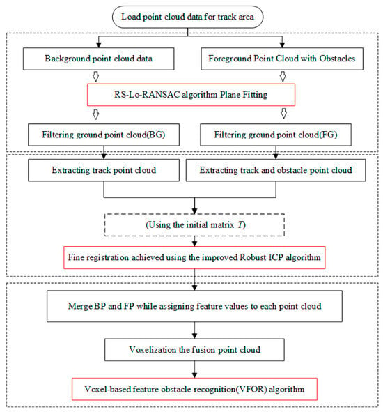
Figure 5.
The flowchart of the whole obstacle detection algorithm.
- (a)
- Large-scale ground point cloud segmentation and railway model extraction using RS-Lo-RANSAC;
- (b)
- Background point cloud (BP) and foreground point cloud (FP) (including obstacles) fine registration using improved Robust ICP;
- (c)
- Obstacle recognition based on VFOR algorithm.
3.1. Large-Scale Ground Point Cloud Segmentation and Railway Track Extraction
After calibrating point cloud coordinates, we obtained a large-scale and detailed point cloud of the scanning area. When installed beside the railway tracks, we can obtain a point cloud with features such as the ground, railway tracks, obstacles, or trains. Our algorithm requires a frame of the obstacle-free point cloud as a background point cloud, while the foreground point cloud has obstacles. We first apply an outlier point filter to handle individual noise for the two input point clouds. Then, we perform plane segmentation on the long-range ground point cloud.
The classic RANSAC [21] algorithm fits the samples by randomly selecting a minimal subset. Points within the defined threshold range of error are considered inliers. The loop’s termination occurs when the probability of losing an internal element set of size m among k samples is lower than a predefined threshold. The selection of the sample size should be as follows:
where represents the likelihood of randomly selecting a minimal sample of points that are considered inliers, represents the theoretical number of points for the inliers, and represents the number of all points in the dataset.
However, the assumption is not always valid because RANSAC cannot guarantee that the sampled points are not contaminated during the random selection process. Therefore, in situations with significant noise, the algorithm is more prone to being affected and typically requires a more substantial number of iterations than the theoretical value.
In the iteration process, can represent a lack of confidence in the correct model estimation. At the same time, can be interpreted as the probability of the model being correctly estimated. represents the correct model parameters, and represents the estimated ones. The error is quantitatively estimated by function . represents the dataset of selected n samples, represents the dataset of samples belonging to inliers, and represents the dataset of samples belonging to outliers. According to [22], Equation (9) can be rewritten as follows:
For some, > 0.
When the probability distributions of internal and external points and noise overlap significantly, assuming that the internal noise follows a Gaussian distribution, the following formula can describe the relationship between the optimal selection of model points with the known signal-to-noise ratio, denoted by .
Following the abovementioned assumptions, Equation (14) follows a quadratic distribution. Based on the experimental findings [20], the optimal sample size (denoted as n*) for reconstructing the model satisfies the following relationship:
To improve the stability of the model, Lo-RANSAC [21,22] introduces a local optimization step. After obtaining the best model so far, it samples and performs local optimization using the inlier points. This process generates a new model with a higher proportion of inliers for subsequent iterations. Experimental results have demonstrated that Lo-RANSAC, which incorporates sample-local optimization, exhibits superior robustness in plane segmentation compared to the classical RANSAC algorithm.
Inspired by the works of [22,23], we have proposed a strategy to enhance the stability and operational efficiency of Lo-RANSAC [24] in ground segmentation while further reducing the impact of noise on model fitting called RS-Lo-RANSAC (Region Select Lo-RANSAC). In the process of fitting the minimum sample model, we incorporated the optimal sample Formula (15) as a reference to guide the fitting process. In the Lo-RANSAC sample fitting process [25], the fitting of the current sample is achieved by randomly selecting a certain number of sample points between the minimum sample and the optimal sample. Therefore, we refer to this process as RS-Lo-RANSAC, indicating the selection of sample points from a specific region. The method consists of the following steps (the pseudocode of the algorithm is shown as Algorithm 1):
- (a)
- Randomly select to sample points within an adaptively determined range capable of fitting the model and employ these points for least squares sample fitting.
- (b)
- Iterate through a loop and perform local optimization when the best model so far is identified, utilizing the Total Least Square (TLS) method to optimize the inlier points of the model.
- (c)
- Implement early termination of iterations based on probabilistic principles. By satisfying certain conditions derived from probability statistics, we can determine when the model has achieved a stable state, allowing for the termination of the iteration process.
| Algorithm 1: RS-Lo-RANSAC algorithm use for ground segmentation and track extraction |
| Input:; |
| Output: |
| do |
| ← randomly |
| calculate the current model |
| caculate the inlier points of the plane |
| then 7: // run Local Optimization do model estimated by TLS inliers then 14: end if 16: end for 17: end if |
The termination condition can be defined as the following:
where represents the number of inlier points within the best model so far, represents the total number of points in the point cloud, and m is the minimum sample fit threshold.
By implementing these steps, our goal is to significantly improve the stability and operational efficiency of Lo-RANSAC in ground segmentation, while minimizing the influence of noise on model fitting.
3.2. Fine Registration of BP and FP
After ground segmentation, we obtained point cloud maps of the respective track regions (BP and FP). We aim to achieve the fine registration of these point cloud maps at this stage.
The Iterative Closest Point (ICP) [26] algorithm is widely used for point cloud registration [27,28]. Its core principle is to iteratively refine a mapping transformation from a source point cloud to a target point cloud. The objective is to find the best alignment between source and target point clouds. The algorithm computes the optimal transformation by minimizing distance metrics such as Euclidean distance or point-to-plane distance. Through iterative updates, the ICP algorithm gradually converges to achieve an accurate registration result:
where = {} P is one of the points in the source point cloud, and = {} Q is one of the points in the target point cloud. is the rotation matrix. is the translation vector. During the iteration process of ICP, several commonly used strategies for finding point-to-point correspondences in point clouds include point-to-point, point-to-line, and point-to-plane [29]. The steps of the traditional ICP algorithm are as follows [30]:
- (a)
- Given an initial source point cloud set P and input set Q, find the subset X in set P that corresponds to a set Y in Q, which can be described as , in which k represents the number of iterations of the ICP and is initialized as zero.
- (b)
- Calculate the mapping matrix based on the point set relation between and , and the mapping matrix is represented as (18):
- (c)
- Apply the mapping matrix to the input source point cloud for pose transformation, , and use point cloud as the input source for the next round. And calculate the mean squared point matching error .
- (d)
- If the value of is less than a certain threshold, exit the loop and consider the current mapping matrix T as the optimal solution. Otherwise, continue iterating until the maximum number of iterations k is reached.
In correspondence step, we usually use the l2-norm to represent the registration error. However, the convergence of the Iterative Closest Point (ICP) algorithm may be hindered by outliers, partial overlap, occlusion, and other issues present in the source and target point clouds. The TrICP algorithm proposed by Chetveriko et al. [31] addresses this problem by introducing the concept of overlap during the iterative process to remove outlier points. Assuming Equation (19) is satisfied in the given scenario of source point set A and target point set B, the computation of overlap allows for filtering out points between the two sets that meet the defined overlap criteria during the iterative process. This helps to minimize the influence of misalignment caused by distant outliers. However, computing the optimal overlap can be computationally expensive.
where represents the overlap defined during the iterative process of TrICP.
The Sparse ICP [32] algorithm improves sparsity in the source point cloud set and target point cloud set by replacing the l2-norm with an lp-norm in the error metric function. The loss function is denoted as (20):
While this does mitigate the penalty for point pairs with significant spatial separation to some extent, it is important to note that the inclusion of the alternating direction method of multipliers (ADMM) in the solution process significantly amplifies the computational complexity.
To overcome the limitations posed by the previously mentioned methods and effectively tackle the challenges arising from partial overlap and outlier points during the registration process, Zhang et al. [33] proposed a novel registration approach. This method incorporates Welsch’s function as a loss function, strategically formulating the correspondence step in the following manner:
where is the indicator function of the special orthogonal group, and is the Welsch’s function, which is denoted as (22):
By introducing a quadratic surrogate function , the problem during the alignment steps is formulated as a weighted least squares problem for the following solution:
In Formula (22), is an independent variable that can control the value of the Welsch’s function, and the specific influence curve can be referred to in Figure 6.
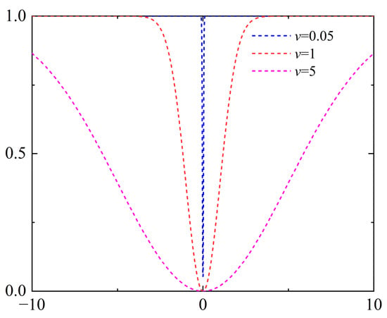
Figure 6.
Welsch’s function.
The weight coefficient is observable, which is associated with the distance between point pairs and follows a Gaussian distribution. Its range is constrained to (0, 1] (As shown in Figure 6). When the distance between the registration point pairs is sufficiently large, the weight diminishes, penalizing outliers and preventing erroneous registration. Conversely, when the weight is small, more point pairs can participate in the registration process, improving precision and robustness. This method can be regarded as a soft-thresholding approach that penalizes points with more significant errors during the iterative procedure, yielding more stable outcomes.
In the iterative registration process, the update strategy and range interval of the Gaussian weight parameter play a crucial role. A well-designed iteration strategy enables more point pairs to be involved in the registration, thereby preventing overfitting and improving the algorithm’s robustness and efficiency. Zhang et al. [33] proposed boundary conditions for based on the assumption that the sampled points in a point cloud have a uniform density. These boundary conditions are defined as 3 (where represents the median of registration errors) according to the three-sigma rule. Additionally, another boundary condition is set as (where represents the median of neighboring points) to enhance the tolerance of sampled points.
During the registration process, starting from one boundary condition, the intermediate transformation matrix’s change is monitored. If this change is below a threshold or the maximum iteration count is reached, the current iteration is terminated, and the weight is reduced by half until reaching the other boundary condition. This iterative approach ensures the fine-tuning of the registration process and achieves optimal results. However, in practical scenarios where the density of the same point cloud varies significantly, the above strategy may not perform well for certain samples and lead to overfitting. To address this issue, we propose a new improved point cloud registration strategy to enhance the usability of the Robust ICP algorithm. This new strategy demonstrates superior efficiency and robustness in test samples.
As shown in Figure 7, the density of point clouds within the point cloud map exhibits significant variation with distance. The original algorithm employed the median of neighbor points in the point cloud map to determine the upper and lower bounds of parameters. Considering this observation, we propose the following enhancements.
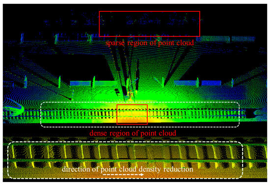
Figure 7.
In large-scale scene applications, the density variation of the point cloud is very significant.
Regarding , we aim to achieve a comprehensive matching relationship while minimizing the number of iterative cycles. To accomplish this, we transform the target point cloud using the mapping matrix and then analyze the resulting relationships after removing outliers. Through this analysis, we determine the maximum difference in the initial transformation of the point cloud, which serves as the definition for .
In the case of , we aim to improve registration point sparsity while adhering to specific constraints. To achieve this, we examine the point density within fixed-threshold neighborhoods in the point cloud map and eliminate any exceptional values. Instead of using a traditional , we adopt the maximum value among all points in the neighborhood. We argue that this strategy yields smoother Gaussian weights across spatial regions, mainly for non-uniform density point cloud maps. This approach increases tolerance towards matching errors while partially constraining the function to deviate from the l0-norm. The intention is to strike a balance between accommodating significant error points and ensuring precise alignment in the results.
Lastly, throughout the iterative process, we have observed that in a specific cycle, when the value of v reaches a fixed point, the last few iterations cease to contribute significantly to achieving precise alignment of the samples. This diminished effect can be attributed to energy convergence. To tackle this issue, we have devised an adaptive iteration strategy based on the convergence energy. This adaptive strategy can be summarized as follows.
The determination to terminate the current iteration is made by continuously monitoring the changes in the convergence energy. By observing this energy metric, we can identify when further iterations will yield diminishing returns in terms of improving alignment accuracy. This approach ensures that the iterative process is dynamically adjusted based on the convergence behavior, thus optimizing the efficiency and effectiveness of the algorithm.
In this case, represents the final convergence energy, stands for the convergence energy during the initial iteration process, and represents our adaptive threshold.
The pseudocode for the key steps of the algorithm is as Algorithm 2:
| Algorithm 2: Improved point-to-point Robust ICP using Welsch’s function |
| Input: : initial transformation; ; : maximum iteration count; : convergence ability of iterative functions; : convergence capability of the previous iteration; : number of iterations; : energy threshold ; Initial |
| do |
| ; |
| do |
| then |
6: else break; 7: end if then break; end if 13: //Using Anderson acceleration; [33,34] 16: ; 17: end while ; 19: end if 21: end while |
3.3. Extracting Voxel Features from Fused Point Clouds
Voxel grids are extensively utilized in the processing of large volumes of data within point clouds [35,36]. Grid-based voxelization, a common technique, is employed to downsample the point cloud data, thereby reducing density and introducing sparsity [37].
In our preceding steps, we employed the RS-Lo-RANSAC algorithm to extract the ground-removed point cloud in source and target point clouds. Subsequently, by employing an improved Robust ICP algorithm, we successfully fused the BG and FG point clouds, resulting in a coherent point cloud representation. Importantly, this fused point cloud incorporates feature labels (for obstacle detection requirements with a minimum size of Acm × Acm × Acm, we usually set the empirical parameter of Voxelsize to (A ± 5) cm) (as shown in Figure 8).

Figure 8.
We use Octree technology to voxelize the fused point cloud. Next, we cycle through each voxel grid to determine whether the point cloud within that grid belongs to the category of obstacles.
We have devised an innovative obstacle recognition algorithm to harness the unique features within the fused point cloud. Our approach incorporates voxelization as a crucial step, dividing the point cloud into fixed-size voxel grids. The size parameter of these voxel grids is directly related to the desired obstacle resolution, denoted by Voxelsize.
First, we voxelize the fused point cloud map using a voxel grid with a side length of Voxelsize. The index established in the XYZ order is . In the point retrieval process, we leverage Octree [38] to expedite this procedure.
Subsequently, according to Formulas (27) and (28), we analyzed the point cloud within each voxel grid . This analysis allows us to determine whether a particular voxel grid corresponds to an obstacle grid. Expressing this relationship, we can establish the following:
Here, represent the respective counts of points belonging to the BG and FG within . is a threshold value that correlates with the point cloud density . Meanwhile, denote the heights of points attributed to the BG and FG point clouds in . is associated with the desired height threshold for obstacle detection determined by the experimenter (for obstacle detection requirements with a minimum size of Acm × Acm × Acm, we usually set the empirical parameter of Voxelsize to (A ± 5) cm).
4. Experiment
The configuration of the system with our algorithm is the following: AMD Ryzen 5 5600G with Radeon Graphics, 32 GB RAM and NVIDIA GeForce RTX 3060 Ti.
4.1. Point Cloud Coordinate Correction
In our experiment on precise error coordinate correction, we opted to employ the system operating at a frequency of 50 Hz and an angular resolution of 0.33° for data acquisition and processing. By carefully adjusting the vertical angular resolution, we examined the accuracy of coordinate correction across various angular resolutions and scanning distances.
To calculate the angle compensation for each pulse point, we utilized Equations (5) and (6). We also proposed a measurement of the error between the corrected and original coordinates using the Euclidean distance (). This measurement allowed us to quantify the discrepancy between the two points.
In Figure 9a, we gathered distance measurements at various horizontal positions and elevation angles, maintaining a consistent resolution. The variable point order denotes the sequential sequence of pulses in the horizontal direction. The pulse distance represents the magnitude of the detection distance, and then we will be able to quantitatively observe the extent of error correction at this detection distance. The maximum distance we captured in this instance was 9.5 m. In Figure 9b, we utilized Formulas (4)–(6) to rectify errors in each pulse. Notably, the compensation’s effectiveness becomes more prominent as the elevation and lateral angles increase. The maximum effective compensation occurred at a lateral angle of 138° and an elevation angle of 58.26°, resulting in an approximate correction of 27 mm. In the provided data, even the smallest error was compensated for by 10 mm. Figure 9c exemplifies the linear correlation between different elevation angle resolutions and their associated compensatory effects while upholding a constant horizontal angle resolution. In Figure 9d, we utilized a control system with different elevation scan speeds to enable data acquisition at a fixed position (30°). Additionally, we applied coordinate correction to the collected data at various elevation angle resolutions. This implies that when we employ different scanning speeds, varying degrees of compensation will be near the same scan line position. Specifically, higher scanning speeds result in more significant compensation.
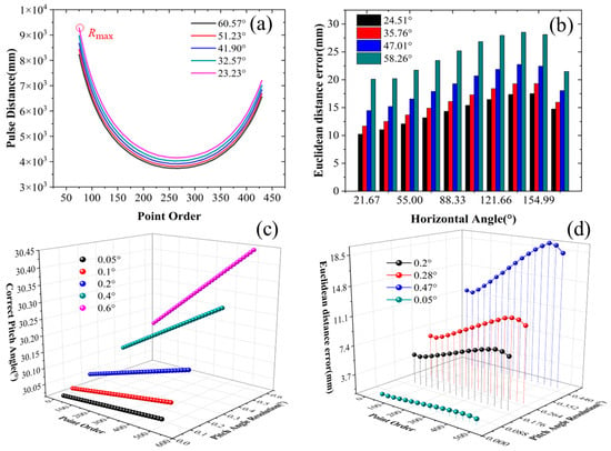
Figure 9.
(a) Pulse distance R in different scanning lines ( = 0.33°, = 0.1°); (b) at four random pitch angles using Formula (6); (c) trend plot of variations for different values of ( = 0.33°, = 30°); (d) for different values of ( = 0.33°, = 30°).
The result of the quantified correction effect demonstrates a noteworthy enhancement in the calibration of three-dimensional coordinates for the measured points, validating the effectiveness of our correction strategy.
4.2. RS-Lo-RANSAC
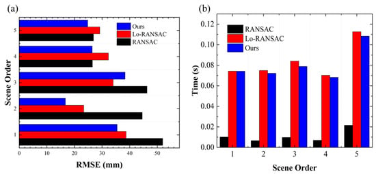
We collected five scenarios from our constructed experimental site to enable ground point cloud segmentation (Figure 10). During the evaluation of our proposed algorithm, we focused on three critical evaluation criteria:
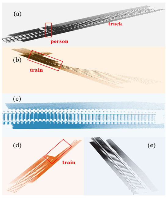
Figure 10.
Five random scenes for ground segmentation: (a) Person on the track (point cloud count n = 120 k); (b) train with significant planar interference (n = 120 k); (c) simple track background (n = 120 k); (d) small planar train at a distance (n = 120 k); (e) dense point cloud background (n = 180 k).
- (a)
- Level of visualization achieved in extracting regions along the track of the point cloud.
- (b)
- The computational efficiency of the algorithm was measured by its execution time.
- (c)
- The accuracy of ground segmentation was assessed by calculating the Root Mean Square Error (RMSE).
The RMSE for the algorithm is calculated as follows:
Here, represents the vertical distance from each point in the sample to the plane model, and represents the number of all points in the sample. Lower RMSE values generally indicate better algorithm results.
We tested three different algorithms: the traditional RANSAC, Lo-RANSAC, and our proposed algorithm. When (Distance Threshold) was set at 80 and (maximum number of iterations) was set to 1000, the traditional RANSAC algorithm exhibited faster execution speed than both Lo-RANSAC and our algorithm, as shown in the results depicted in Figure 11. However, our algorithm, an improvement based on the Lo-RANSAC algorithm, demonstrated some enhancements in terms of execution speed.
In order to further verify the stability of the algorithm for ground segmentation in practical complex situations, we introduced an “interference plane” by moving trains (Figure 12a,e,i) and set three different parameters (ϵ = 80, 85, and 90; k = 2000; η = 0.05) in Scene A, B, and C. The RMSE and Time Cost of the three algorithms are recorded in Table 1. It can be seen that in the case of low intervention in the “interference plane” (Scene A and B), the traditional RANSAC algorithm performs better than the other two algorithms in RMSE and Time, while our RS-Lo-RANSAC algorithm always achieves better results than the Lo-RANSAC algorithm. However, in the presence of severe interference planes (Figure 12i), RANSAC exhibits poor performance that cannot be segmented (Figure 12j), while the other two algorithms have completed the predetermined tasks. Overall, the RS-Lo-RANSAC algorithm performs more stably in various situations, indicating that our algorithm strategy is suitable for segmentation tasks in large-scale point clouds. The phenomenon of RANSAC algorithm segmentation failure may be due to the limitation of iteration times and the uncertainty of non-target-planar noise, which affects the convergence of the RANSAC algorithm. Meanwhile, our algorithm exhibited improved RMSE compared to the Lo-RANSAC algorithm in the majority of samples and showed a reduction in the algorithm’s runtime. By comparing the results in Table 1, our algorithm showcased significant improvements in robustness, particularly in specific scenarios, compared to the RANSAC and Lo-RANSAC algorithms. This can be attributed to our sample selection strategy, which enhanced the algorithm’s capability to handle non-planar noise and overall robustness.
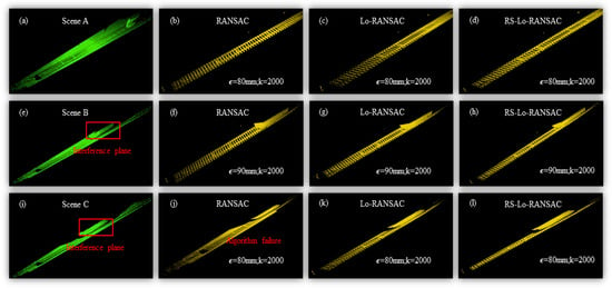
Figure 12.
We introduced different interference planes to test the segmentation performance of algorithms and set their respective thresholds in different scenarios. Among them, (a–d) are the original point clouds in Scene A and the processing results of the three segmentation algorithms; (e–h) are the original point cloud and the processing results of three segmentation algorithms in Scene B. Similarly, (i–l) are the situations of Scene C.

Table 1.
We collected the RMSE and Time Cost performance of RANSAC, Lo-RANSAC, and RS-Lo-RANSAC algorithms under different threshold (ϵ = 80, 85, and 90) settings in Scene A, B, and C, to measure the effectiveness of the three algorithms for ground segmentation when interference planes appear.
By incorporating the proposed RS-Lo-RANSAC algorithm steps, we successfully improved upon the Lo-RANSAC algorithm while optimizing its execution speed. In our experiments, our algorithm consistently outperformed the traditional RANSAC and Lo-RANSAC algorithms regarding noise resistance in most scenarios. This enhanced robustness allowed us to obtain superior point cloud data in the track area of real-world scenes, significantly reducing the workload and complexity of subsequent algorithmic tasks (for more test data, refer to Table 2).

Table 2.
The enhancement of RMSE in Lo-RANSA and RS-Lo-RANSAC compared to traditional RANSAC used for ground segmentation in various scenarios. The “RANSAC (mm)” line represents the specific value of RMSE calculated using the RANSAC algorithm, and the following two lines represent the percentage increase in RMSE obtained by the Lo-RANSAC and RS-Lo-RANSAC algorithms (the calculation formula is the following: ).
4.3. Improved Robust ICP
Regarding the improved Robust ICP algorithm proposed, a subset of test scenarios was randomly selected to evaluate the algorithm’s performance based on the following metrics (the visualization process is shown in Figure 13):
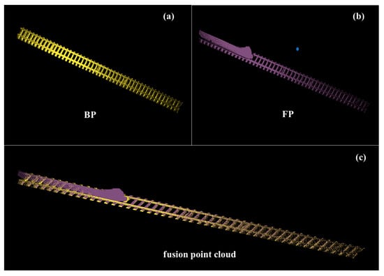
Figure 13.
(a) Background point cloud after ground segmentation with RS-Lo-RANSAC; (b) foreground point cloud after the same steps; (c) in the registration steps, we will use the improved Robust ICP algorithm to register and fuse the point clouds of (a,b).
- (a)
- Convergence ability was measured by the variation of the Gaussian weights during the correspondence step. This variation can be expressed as follows:
- (b)
- Mean Square Error (MSE) at each iteration:
- (c)
- The runtime t of the algorithm.
- (d)
- The interval between fixed marker points in the foreground and background point clouds indicates the level of registration, and the smaller , the better the registration effect.
The results showed that our algorithm effectively controlled the number of iterations during the initial round of updating the Gaussian weights in the test scenarios, significantly reducing runtime. We observed that the strategy used by Zhang et al. [31] for point cloud scenarios with significant density variations, as shown in Figure 14, had slow convergence for the first iteration. Excessive iterations had a minimal impact on reducing the MSE and resulted in excessive registration, leading to decreased algorithm efficiency. However, as Figure 15a,b demonstrated, our proposed strategy effectively mitigated this phenomenon. Moreover, while ensuring that the MSE remained nearly the same or slightly improved, Figure 15c illustrates the improved runtime achieved by our algorithm, with a maximum improvement of 1.9 s in specific scenarios. Furthermore, although traditional ICP exhibited faster runtime efficiency in most samples, it showed instability in some instances. Figure 15d demonstrates the comparison between our algorithm and Robust ICP in these five scenarios, where the MSE was nearly equal. Notably, our algorithm further improved the registration time of the samples.
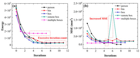
Figure 14.
(a) Convergence of energy during the correspondence step of Robust ICP; (b) trend of MSE caused by Robust ICP.
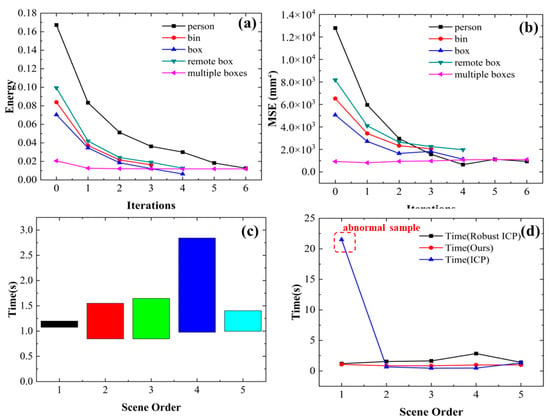
Figure 15.
(a) Convergence trend of energy during initial iterations under our convergence strategy; (b) trend of MSE during the first iteration process under our convergence strategy; (c) comparison of runtime between our algorithm and Robust ICP in five random scenarios (different colors represent five different testing scenarios, while the width on the vertical axis represents the time difference between the two algorithms); (d) registration time comparison among traditional ICP algorithm, Robust ICP algorithm, and our algorithm in five random scenarios.
Furthermore, we collected a frame of background and foreground point clouds and performed ground segmentation through the aforementioned steps (Figure 16a). We marked a pair of labeled points in the foreground and background point clouds, and then used ICP, GICP (Generalized ICP) [39], NDT (Normal Distribution Transform) [40], RICP (Robust ICP) [33] strategies, and our registration algorithm to register and mark . Our strategy achieved the best value of 3.342 cm, indicating that our algorithm demonstrated better registration performance on the sample. At the same time, we calculated the registered MSE and Time Cost in Table 3. Our algorithm also achieved significant advantages in terms of runtime and MSE, especially in terms of runtime. Only 0.38 s were used, achieving the best performance among all tested algorithms.
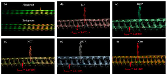
Figure 16.
(a) We selected a foreground point cloud and a background point cloud for a scene and registered them using ICP, GICP, NDT, RICP algorithms (b–f), and our algorithm. Then we calibrated the of the corresponding point pairs.

Table 3.
Statistical analysis of MSE, Time Cost, and performance of samples after different registration strategies with Figure 16a.
4.4. VFOR
In order to further illustrate the quantitative impact of errors in the key links of our algorithm based on the experimental results, we used the RMSE of the RS-Lo-RANSAC algorithm as the benchmark and calculated the error of the Lo-RANSAC algorithm and the error of the RANSAC algorithm. Next, we used the of our Improved Robust ICP algorithm as the benchmark during the registration process and calculated the of the ICP algorithm, the of the GICP algorithm, the of the NDT algorithm, and the of the RICP algorithm. And the results of each combination algorithm were calibrated by combining them. In Figure 17, the red box represents the sample obstacle we placed for identification, while the yellow box represents the noise cluster that was incorrectly identified and the blue box represents the unrecognized obstacle.
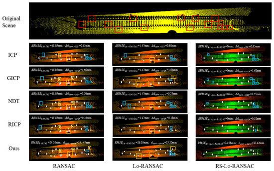
Figure 17.
The impact of errors and on our results. The red boxes in the Original Scene represent the 15 boxes we placed (15 cm × 15 cm × 15 cm). Each column of RANSAC, Lo-RANSAC, and RS-Lo-RANSAC represents the results of different registration algorithms after the corresponding segmentation algorithms. The yellow box represents noise clusters, and the blue box represents undetected boxes. The point cloud of the track area after ground segmentation is marked with green point clouds in the RS-Lo-RANSAC column.
In Figure 17, we annotated the 15 boxes that should theoretically be detected in the Original Scene. The running results of the algorithm combination are shown in Figure 17. It is worth noting that due to the influence of the ground segmentation algorithm on the registration results, our registration results of RANSAC and Lo-RANSAC (33.47 mm and 33.50 mm) are slightly larger than the result of 33.42 mm of our RS-Lo-RANSAC algorithm. In RS-Lo-RANSAC, we prominently marked the track point cloud after ground segmentation using green point clouds. It is evident that we did not see any noise clusters (yellow boxes) after the RS-Lo-RANSAC algorithm segmented the ground, which can be understood as the impact of error on the results (the correct ground segmentation strategy resulted in a smaller and reduced the probability of noise clusters appearing). However, different registration algorithms have a greater impact on the omission of obstacle detection (blue box). When the RS-Lo-RANSAC algorithm is used to correctly segment the ground, as the registration error decreases, it leads to a higher detection rate (with fewer blue boxes), which can be attributed to the quantitative description of registration errors on our results. Based on our current experience, in order to reduce the impact of errors on the results in each step, we need to control the range of error results as follows: is ±3 mm, and the control for should be ±0.05 mm (experienced parameter).
Subsequently, we conducted more extensive testing. We evaluated the algorithm’s ability to recognize obstacles such as people, trains, and cardboard boxes at random locations adjacent to and on the tracks. The algorithm workflow is outlined as follows.
We utilized Table 4, which contains various types of obstacles in our test dataset, to demonstrate the algorithm’s recognition performance for these obstacles. We conducted 100 tests on each obstacle at each position, and the percentage represents the number of times the obstacle was successfully detected. Suppose the intruding point cloud group is significantly large and impacts the RS-Lo-RANSAC and improved Robust ICP steps. We adopted the most effective track extraction model M* and mapping matrix T* from previous continuous runs. The experimental results suggest that our algorithm performs well in handling point cloud processing, even when dealing with more giant obstacles. Regarding recognizing comparatively more minor obstacles, it achieves a detection range of approximately 50 m for threshold obstacles measuring 15 cm × 15 cm ×15 cm. Figure 18 shows the final visualization result of our algorithm.

Table 4.
Summary of our algorithm’s detection capabilities for different obstacles in the experimental field.
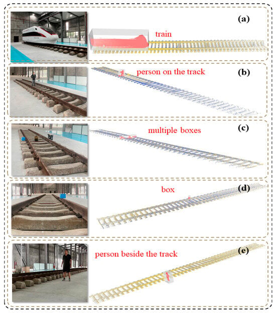
Figure 18.
The final visualization result of the algorithm operation is displayed, where the photo is our actual scene photo, and the red point cloud in the transparent cube is the obstacle point cloud detected by our algorithm. The objects are manually labeled as the types of obstacles in red font: (a) stationary train (large obstacle); (b) human obstacle (1.7 m) located 15 m away from the lidar system; (c) three box obstacles (20 cm3, 25 cm3, and 30 cm3) located 10 m away from the system; (d) single box obstacle (20 cm3) located 5 m away from the system; (e) human obstacle (1.7 m) located alongside the track.
5. Conclusions
Ensuring the safety of railway tracks against obstacles is a paramount task. In this study, we have devised a specialized 3D mechanical lidar system explicitly designed for obstacle detection. To reconstruct objects’ 3D information precisely, we meticulously quantified and calibrated the point cloud coordinate transformation relationship through thorough analysis.
Once we obtained high-precision point cloud data of the scene, we developed a comprehensive set of obstacle detection algorithms encompassing the following key steps:
- (a)
- Ground filtering and track extraction based on RS-Lo-RANSAC;
- (b)
- Fusion of the BP and the FP using an improved Robust ICP;
- (c)
- Obstacle recognition based on voxel features extracted from the fused point cloud map.
We have optimized each algorithm step for robustness and speed, resulting in stable testing in our experimental scenarios. To evaluate the effectiveness of our system and algorithm, we conducted tests on obstacle size and distance within our constructed test site. The results demonstrated the exceptional performance of our algorithm in detecting intruding obstacles such as trains, pedestrians, and cardboard boxes under various test scenarios.
According to the current algorithm operation results, under continuous rainfall weather conditions, the algorithm may be disturbed. In the future, we will strive to solve this limitation. As part of our future work, we will study the algorithm’s robustness in the face of perturbations and assess its effectiveness in adverse weather conditions such as rain, snow, and fog. Meanwhile, due to our algorithm being based on large-scale ground segmentation considerations, it is suitable for processing static point clouds containing large-scale ground. We will further expand the algorithm to more diverse scenarios, such as key highways, railway intersections, tunnels, and flat aircraft runway datasets.
Author Contributions
Conceptualization, Z.N. and G.Z.; methodology, Z.N.; writing—original draft preparation, X.Z.; writing—review and editing, X.Z. and X.L.; supervision, X.L.; funding acquisition, Y.Y. All authors have read and agreed to the published version of the manuscript.
Funding
This work was financially supported by the National Natural Science Foundation of China (No.62275244). And the CAS Project for Young Scientists in Basic Research, Grant No. YSBR-065, National Natural Science Foundation of China (No. 62225507, No. U2033211, No. 62175230, and No. 62175232), Scientific Instrument Developing Project of the Chinese Academy of Sciences, Grant No. YJKYYQ20200001, National Key R&D Program of China (No. 2022YFB3607800, No. 2022YFB3605800, and No. 2022YFB4601501), and the Key Program of the Chinese Academy of Sciences (ZDBS-ZRKJZ-TLC018).
Data Availability Statement
The authors confirm that the data supporting the findings of this study are available within the article.
Conflicts of Interest
Author Xu Zhang was employed by the company Shenghong (Taizhou) Laser Technology Co. Ltd. The remaining authors declare that the research was conducted in the absence of any commercial or financial relationships that could be construed as a potential conflict of interest.
References
- Ye, T.; Zhang, X.; Zhang, Y.; Liu, J. Railway Traffic Object Detection Using Differential Feature Fusion Convolution Neural Network. IEEE Trans. Intell. Transp. Syst. 2021, 22, 1375–1387. [Google Scholar] [CrossRef]
- Pan, H.; Li, Y.; Wang, H.; Tian, X. Railway Obstacle Intrusion Detection Based on Convolution Neural Network Multitask Learning. Electronics 2022, 11, 2697. [Google Scholar] [CrossRef]
- Kapoor, R.; Goel, R.; Sharma, A. An intelligent railway surveillance framework based on recognition of object and railway track using deep learning. Multimed. Tools Appl. 2022, 81, 21083–21109. [Google Scholar] [CrossRef] [PubMed]
- Ristic-Durrant, D.; Franke, M.; Michels, K. A Review of Vision-Based On-Board Obstacle Detection and Distance Estimation in Railways. Sensors 2021, 21, 3452. [Google Scholar] [CrossRef] [PubMed]
- Dodge, D.; Yilmaz, M. Convex Vision-Based Negative Obstacle Detection Framework for Autonomous Vehicles. IEEE Trans. Intell. Veh. 2023, 8, 778–789. [Google Scholar] [CrossRef]
- Perić, S.; Milojković, M.; Stan, S.-D.; Banić, M.; Antić, D. Dealing with Low Quality Images in Railway Obstacle Detection System. Appl. Sci. 2022, 12, 3041. [Google Scholar] [CrossRef]
- Kyatsandra, A.K.; Saket, R.K.; Kumar, S.; Sarita, K.; Vardhan, A.S.S.; Vardhan, A.S.S. Development of TRINETRA: A Sensor Based Vision Enhancement System for Obstacle Detection on Railway Tracks. IEEE Sens. J. 2022, 22, 3147–3156. [Google Scholar] [CrossRef]
- Shao, W.; Zhang, H.; Wu, Y.; Sheng, N.; Zhou, S. Application of fusion 2D lidar and binocular vision in robot locating obstacles. J. Intell. Fuzzy Syst. 2021, 41, 4387–4394. [Google Scholar] [CrossRef]
- Miao, Y.; Tang, Y.; Alzahrani, B.A.; Barnawi, A.; Alafif, T.; Hu, L. Airborne Lidar Assisted Obstacle Recognition and Intrusion Detection Towards Unmanned Aerial Vehicle: Architecture, Modeling and Evaluation. IEEE Trans. Intell. Transp. Syst. 2021, 22, 4531–4540. [Google Scholar] [CrossRef]
- Wang, D.; Watkins, C.; Xie, H. MEMS Mirrors for Lidar: A review. Micromachines 2020, 11, 456. [Google Scholar] [CrossRef]
- Zheng, L.; Zhang, P.; Tan, J.; Li, F. The Obstacle Detection Method of UAV Based on 2D Lidar. IEEE Access 2019, 7, 163437–163448. [Google Scholar] [CrossRef]
- Amaral, V.; Marques, F.; Lourenço, A.; Barata, J.; Santana, P. Laser-Based Obstacle Detection at Railway Level Crossings. J. Sens. 2016, 2016, 1719230. [Google Scholar] [CrossRef]
- Xie, D.; Xu, Y.; Wang, R. Obstacle detection and tracking method for autonomous vehicle based on three-dimensional LiDAR. Int. J. Adv. Robot. Syst. 2019, 16, 1729881419831587. [Google Scholar] [CrossRef]
- Sun, Y.; Zuo, W.; Huang, H.; Cai, P.; Liu, M. PointMoSeg: Sparse Tensor-Based End-to-End Moving-Obstacle Segmentation in 3-D Lidar Point Clouds for Autonomous Driving. IEEE Robot. Autom. Lett. 2021, 6, 510–517. [Google Scholar] [CrossRef]
- Gao, F.; Li, C.; Zhang, B. A Dynamic Clustering Algorithm for Lidar Obstacle Detection of Autonomous Driving System. IEEE Sens. J. 2021, 21, 25922–25930. [Google Scholar] [CrossRef]
- Anand, B.; Senapati, M.; Barsaiyan, V.; Rajalakshmi, P. LiDAR-INS/GNSS-Based Real-Time Ground Removal, Segmentation, and Georeferencing Framework for Smart Transportation. IEEE Trans. Instrum. Meas. 2021, 70, 1–11. [Google Scholar] [CrossRef]
- Fang, J.; Zhou, D.; Yan, F.; Zhao, T.; Zhang, F.; Ma, Y.; Wang, L.; Yang, R. Augmented Lidar Simulator for Autonomous Driving. IEEE Robot. Autom. Lett. 2020, 5, 1931–1938. [Google Scholar] [CrossRef]
- Chen, J.; Kira, Z.; Cho, Y.K. LRGNet: Learnable Region Growing for Class-Agnostic Point Cloud Segmentation. IEEE Robot. Autom. Lett. 2021, 6, 2799–2806. [Google Scholar] [CrossRef]
- Ci, W.Y.; Xu, T.; Lin, R.Z.; Lu, S.; Wu, X.L.; Xuan, J.Y. A Novel Method for Obstacle Detection in Front of Vehicles Based on the Local Spatial Features of Point Cloud. Remote Sens. 2023, 15, 1044. [Google Scholar] [CrossRef]
- Li, J.; Li, R.; Wang, J.Z.; Yan, M. Obstacle information detection method based on multiframe three-dimensional lidar point cloud fusion. Opt. Eng. 2019, 58, 116102. [Google Scholar] [CrossRef]
- Fischler, M.A.; Bolles, R.C. Random sample consensus. Commun. ACM 1981, 24, 381–395. [Google Scholar] [CrossRef]
- Sangappa, H.K.; Ramakrishnan, K.R. A probabilistic analysis of a common RANSAC heuristic. Mach. Vis. Appl. 2018, 30, 71–89. [Google Scholar] [CrossRef]
- Chum, O.; Matas, J.; Kittler, J. Locally optimized RANSAC. In Proceedings of the Pattern Recognition: 25th DAGM Symposium, Magdeburg, Germany, 10–12 September 2003; pp. 236–243. [Google Scholar]
- Huang, X.; Walker, I.; Birchfield, S. Occlusion-aware multi-view reconstruction of articulated objects for manipulation. Robot. Auton. Syst. 2014, 62, 497–505. [Google Scholar] [CrossRef]
- Jiang, S.; Jiang, W.; Li, L.; Wang, L.; Huang, W. Reliable and Efficient UAV Image Matching via Geometric Constraints Structured by Delaunay Triangulation. Remote Sens. 2020, 12, 3390. [Google Scholar] [CrossRef]
- Estépar, R.; Brun, A.; Westin, C.-F. Robust Generalized Total Least Squares Iterative Closest Point Registration. In Proceedings of the Medical Image Computing and Computer-Assisted Intervention–MICCAI 2004: 7th International Conference, Saint-Malo, France, 26–29 September 2004; pp. 234–241. [Google Scholar]
- Zhong, S.; Guo, M.; Lv, R.; Chen, J.; Xie, Z.; Liu, Z. A Robust Rigid Registration Framework of 3D Indoor Scene Point Clouds Based on RGB-D Information. Remote Sens. 2021, 13, 4755. [Google Scholar] [CrossRef]
- Senin, N.; Colosimo, B.M.; Pacella, M. Point set augmentation through fitting for enhanced ICP registration of point clouds in multisensor coordinate metrology. Robot. Comput.-Integr. Manuf. 2013, 29, 39–52. [Google Scholar] [CrossRef]
- He, Y.; Yang, J.; Hou, X.; Pang, S.; Chen, J. ICP registration with DCA descriptor for 3D point clouds. Opt Express 2021, 29, 20423–20439. [Google Scholar] [CrossRef] [PubMed]
- Li, W.; Song, P. A modified ICP algorithm based on dynamic adjustment factor for registration of point cloud and CAD model. Pattern Recognit. Lett. 2015, 65, 88–94. [Google Scholar] [CrossRef]
- Chetverikov, D.; Stepanov, D.; Krsek, P. Robust Euclidean alignment of 3D point sets: The trimmed iterative closest point algorithm. Image Vis. Comput. 2005, 23, 299–309. [Google Scholar] [CrossRef]
- Bouaziz, S.; Tagliasacchi, A.; Pauly, M. Sparse Iterative Closest Point. Elev. Eurographics/Acmsiggraph Symp. Geom. Process. 2013, 32, 113–123. [Google Scholar] [CrossRef]
- Zhang, J.; Yao, Y.; Deng, B. Fast and Robust Iterative Closest Point. IEEE Trans. Pattern Anal. Mach. Intell. 2022, 44, 3450–3466. [Google Scholar] [CrossRef] [PubMed]
- Walker, H.F.; Ni, P. Anderson Acceleration for Fixed-Point Iterations. SIAM J. Numer. Anal. 2011, 49, 1715–1735. [Google Scholar] [CrossRef]
- Kong, S.; Shi, F.; Wang, C.; Xu, C. Point Cloud Generation from Multiple Angles of Voxel Grids. IEEE Access 2019, 7, 160436–160448. [Google Scholar] [CrossRef]
- Shi, G.; Wang, K.; Li, R.; Ma, C. Real-Time Point Cloud Object Detection via Voxel-Point Geometry Abstraction. IEEE Trans. Intell. Transp. Syst. 2023, 24, 5971–5982. [Google Scholar] [CrossRef]
- Tzamarias, D.E.O.; Chow, K.; Blanes, I.; Serra-Sagrista, J. Fast Run-Length Compression of Point Cloud Geometry. IEEE Trans. Image Process 2022, 31, 4490–4501. [Google Scholar] [CrossRef] [PubMed]
- Koh, N.; Jayaraman, P.K.; Zheng, J. Truncated octree and its applications. Vis. Comput. 2021, 38, 1167–1179. [Google Scholar] [CrossRef]
- Young, M.; Pretty, C.; McCulloch, J.; Green, R. Sparse point cloud registration and aggregation with mesh-based generalized iterative closest point. J. Field Robot. 2021, 38, 1078–1091. [Google Scholar] [CrossRef]
- Das, A.; Waslander, S.L. Scan registration using segmented region growing NDT. Int. J. Robot. Res. 2014, 33, 1645–1663. [Google Scholar] [CrossRef]
Disclaimer/Publisher’s Note: The statements, opinions and data contained in all publications are solely those of the individual author(s) and contributor(s) and not of MDPI and/or the editor(s). MDPI and/or the editor(s) disclaim responsibility for any injury to people or property resulting from any ideas, methods, instructions or products referred to in the content. |
© 2024 by the authors. Licensee MDPI, Basel, Switzerland. This article is an open access article distributed under the terms and conditions of the Creative Commons Attribution (CC BY) license (https://creativecommons.org/licenses/by/4.0/).