Article

Comparison between Satellite Derived Solar-Induced Chlorophyll Fluorescence, NDVI and kNDVI in Detecting Water Stress for Dense Vegetation across Southern China

1
Hainan Geomatics Center of Ministry of Natural Resources, Haikou 570203, China
2
Key Laboratory of Ecosystem Network Observation and Modeling, Institute of Geographic and Nature Resources Research, Chinese Academy of Sciences, Beijing 100101, China
*
Author to whom correspondence should be addressed.
These authors contributed equally to this work.
Remote Sens. 2024, 16(10), 1735; https://doi.org/10.3390/rs16101735
Submission received: 13 January 2024 / Revised: 11 April 2024 / Accepted: 23 April 2024 / Published: 14 May 2024

Abstract

:
In the context of global climate change and the increase in drought frequency, monitoring and accurately assessing the impact of hydrological process limitations on vegetation growth is of paramount importance. Our study undertakes a comprehensive evaluation of the efficacy of satellite remote sensing vegetation indices—Normalized Difference Vegetation Index (MODIS NDVI product), kernel NDVI (kNDVI), and Solar-Induced chlorophyll Fluorescence (GOSIF product) in this regard. Initially, we applied the LightGBM-Shapley additive explanation framework to assess the influencing factors on the three vegetation indices. We found that Vapor Pressure Deficit (VPD) is the primary factor affecting vegetation in southern China (18°–30°N). Subsequently, using Gross Primary Productivity (GPP) estimates from flux tower sites as a performance benchmark, we evaluated the ability of these vegetation indices to accurately reflect vegetation GPP changes during drought conditions. Our findings indicate that SIF serves as the most effective surrogate for GPP, capturing the variability of GPP during drought periods with minimal time lag. Additionally, our study reveals that the performance of kNDVI significantly varies depending on the estimation of different kernel parameters. The application of a time-heuristic estimation method could potentially enhance kNDVI’s capacity to capture GPP dynamics more effectively during drought periods. Overall, this study demonstrates that satellite-based SIF data are more adept at monitoring vegetation responses to water stress and accurately tracking GPP anomalies caused by droughts. These findings not only provide critical insights into the selection and optimization of remote sensing vegetation product but also offer a valuable framework for future research aimed at improving our monitoring and understanding of vegetation growth status under climatic changes.

1. Introduction

In the current narrative of global climate change, ecosystems are increasingly vulnerable to various challenges. Foremost among these is drought, a critical natural phenomenon projected to escalate in frequency, duration, and intensity in the upcoming years [1]. The impacts of drought extend beyond the mere reduction of water resources, which significantly influences terrestrial ecosystems, particularly affecting vegetation growth and the stability of plant community. While a universal definition of drought remains elusive, it is typically classified into four categories: meteorological, agricultural (soil moisture), hydrological, and socio-economic droughts [2,3]. Each category interacts with vegetation uniquely. For instance, decreased soil moisture directly hinders plant growth, whereas meteorological drought indirectly affects vegetation by altering the climatic conditions [4,5]. The growth stage of vegetation has a significant impact on the response of NDVI. In the early growth stage, there is less vegetation coverage and lower NDVI values; As vegetation growth and coverage increase, NDVI values increase. In the mature stage, NDVI values may reach high values, reflecting high vegetation density and health status. In the middle and later stages of the lifecycle, although vegetation begins to decline, the sensitivity of NDVI values decreases due to the high vegetation coverage, making it difficult to capture vegetation growth dynamics in a timely manner. kNDVI provides improved sensitivity for capturing changes in vegetation growth stages, especially in the mid to late stages of vegetation growth. Due to its data processing method, kNDVI can more accurately reflect minor changes in vegetation growth and aging processes.
Satellite remote sensing technology has become indispensable for monitoring and assessing the impact of drought on ecosystems [6]. The Normalized Difference Vegetation Index (NDVI) has been the predominant proxy index for vegetation monitoring, which leverages the spectral characteristics of vegetation in the near-infrared and red bands to detect photosynthetically active substances [7,8]. However, NDVI may experience saturation in regions of dense vegetation or during seasonal peaks [9]. The kernel Normalized Difference Vegetation Index (kNDVI) offers a non-linear enhancement of NDVI, capturing a broader range of differences between the near-infrared and red bands [10]. This makes kNDVI more adept at estimating key vegetation physiological parameters, such as Leaf Area Index (LAI), Gross Primary Productivity (GPP), leaf and canopy chlorophyll content, and vegetation light use efficiency, as well as in applications like flux tower-level latent heat measurements [11].
Solar-Induced Chlorophyll Fluorescence (SIF) provides insights into the dynamic shifts in plant photosynthesis. Unlike indices based on vegetation reflectance, SIF directly tracks the efficiency of vegetation photosynthesis [12,13]. However, the effectiveness of SIF varies across different ecosystems and climatic conditions. For example, its sensitivity to meteorological drought is especially pronounced in arid areas characterized by high temperatures during the growing season and low vegetation productivity [14]. While comparisons between SIF and traditional vegetation indices in drought monitoring have been conducted, the performance of kNDVI in such comparisons has been limited [15]. Thus, this study aims to address this gap by evaluating the responsiveness of SIF, NDVI and kNDVI in tracking changes in soil moisture and vapor pressure deficit, and further enhances our understanding of vegetation physiological status under water stress conditions.
Statistical techniques (e.g., correlation and regression analyses) [16,17,18] and ecosystem simulation models [19] are commonly employed to assess vegetation response to water stress. Traditional statistical methods, however, mainly focused on linear relationships between vegetation changes and their drivers, and correlation does not necessarily denote causation [17]. Ecosystem models, while addressing nonlinear and dynamic aspects of vegetation growth under water deficiency, require numerous parameter settings, which may introduce potential uncertainties. Machine learning approaches, particularly those based on decision tree models, circumvent the need for predetermined functional forms between driving factors and responses. They efficiently manage multiple input variables and pinpoint key influencing factors, thus gaining popularity for analyzing and predicting vegetation dynamics [20,21,22]. LightGBM, a distributed gradient boosting framework based on decision tree algorithms, stands out for its enhanced efficiency and speed compared to other tree-based models [23]. To analyze the response of different vegetation indices to water resource variations, this study utilizes LightGBM to construct regression models of environmental factors and vegetation indices, with integrating the Shapley Additive Explanations (SHAP) method via TreeExplainer for model interpretation. Traditional machine learning models often lack transparency in explaining individual predictions or decisions. The SHAP approach, leveraging TreeExplainer, overcomes this by offering local explanations for model predictions. It can also identify nonlinear interactions between features [24]. By calculating the marginal contribution of each feature to the model output, SHAP can enhance the interpretability of the machine learning models used in this study.
This study first compares the different response of satellite-derived SIF (GOSIF product) and NDVI (MODIS NDVI produdct), kNDVI to long-term changes in water resources, over China’s subtropical areas with high vegetation coverage. Then we explore their interactions with GPP changes during short-term extreme drought events. Generally, our research aims: (1) To compare the sensitivity of SIF, NDVI and kNDVI in detecting the impact of water stress on vegetation growth; (2) To analyze the primary environmental factors influencing vegetation growth using the LightGBM and SHAP method; (3) To evaluate the ability of SIF, NDVI and kNDVI to capture GPP changes in subtropical vegetation under drought stress. By contrasting the performance of SIF, NDVI and kNDVI in long-term responses to changes in water resources and short-term extreme drought events, we aim to clarify the respective strengths and limitations of these indices in drought monitoring and vegetation ecological analysis.

2. Materials and Methods

2.1. Study Area

Our research area encompasses thirteen provinces in the southern China (73–135°E, 18–30°N), including Hainan Island, Guangxi, Guizhou, Yunnan, Sichuan, Chongqing, Guangdong, Hunan, Hubei, Tibet, Jiangxi, Fujian, and Zhejiang. The region’s terrain is complex, including the Hengduan Mountains, Yungui Plateau, Sichuan Basin, Guangxi Basin, and coastal plains, which is higher in the west and lower in the east. The climate is notably diverse and variable. The Tibetan Plateau, due to its high altitude, exhibits a cold and arid plateau climate. The Hengduan Mountain region, with its high mountains and deep valleys, displays diverse climates, ranging from subtropical to cold temperate. The Sichuan Basin, surrounded by mountains, often experiences basin effects, resulting in hot summers and mild winters. The middle and lower reaches of the Yangtze River plain belong to a subtropical monsoon climate, characterized by distinct seasons and abundant precipitation.
The vegetation types in southern China are diverse, ranging from subtropical evergreen broad-leaved forests to cold temperate coniferous forests, exhibiting significant regional geographical differences in vegetation distribution (Figure 1). Vegetation in the Tibetan Plateau is dominated by alpine meadows and grasslands, while the Hengduan Mountain region showcases a variety of vegetation, from subtropical evergreen broad-leaved forests to cold temperate coniferous forests. The vegetation in the Sichuan Basin is mainly composed of crops and subtropical forests, while the middle and lower reaches of the Yangtze River plain are primarily characterized by crops and wetland vegetation, especially extensive areas of rice cultivation (Figure 1).

2.2. MODIS Vegetation Indices

In this study, the monthly optical vegetation indices NDVI and kNDVI for the period 2001–2020 were synthesized based on the daily MODIS Surface Reflectance (SR) product MOD09A1 V6 [25], using monthly averaged method. These products have a spatial resolution of 500 m. The kNDVI, as proposed by Camps-Valls et al. [10], is a novel index designed to address the saturation effects often encountered with NDVI in high-biomass regions. It incorporates kernel methods to effectively handle the non-linear relationships present in vegetation reflectance data, thus enhancing the performance of vegetation indices in areas with dense biomass.
The kNDVI uses a Gaussian kernel function to modify the NDVI calculation, allowing for a more accurate representation of biomass changes in densely vegetated areas. The calculation formula for kNDVI is given by:
k N D V I = tanh n r 2 σ 2
In this formula, (σ) is typically simplified for ease of calculation, set as the average of the Near-Infrared (NIR) and red reflectance, i.e., (σ = 0.5 ∗ (n + r)). However, as indicated by research from Wang et al., this oversimplification can reduce the effectiveness of kNDVI, suggesting that adjustments to σ should be made for specific applications [11]. In this study, a distance heuristic estimation method is employed to estimate the (σ) parameter. This method calculates (σ) based on the average distance between all pixels in the region:
σ = N 1 i N N I R i r e d i
Given that kNDVI is significantly influenced by non-vegetated area pixels [11], we applied the pixel quality assurance (QA) layer of MOD09A1 to identify and exclude pixels marked as clouds, cloud shadows, aerosols, and snow, ensuring the reliability of the kNDVI calculations in our study.

2.3. Solar-Induced Chlorophyll Fluorescence

Solar-induced chlorophyll fluorescence (SIF) data were derived from the global monthly GOSIF dataset (https://globalecology.unh.edu/data/GOSIF.html, accessed on 1 December 2023) [26]. GOSIF was developed using a data-driven approach, based on discrete OCO-2 SIF observation data, medium-resolution imaging spectroradiometer (MODIS) remote sensing data, and meteorological reanalysis data, covering the period from 2001 to 2020 with a spatial resolution of 0.05°. The temporal and spatial resolutions of the GOSIF dataset are monthly and 0.05 × 0.05°, respectively.

2.4. Climate Datasets

The TerraClimate dataset is an essential component in this study. It provides comprehensive monthly climate and climatic water balance data for the global terrestrial surface, spanning the period 1958–2019. This dataset is commonly used in global-scale ecological and hydrological studies, which require both high spatial resolution and temporal variability. The TerraClimate was developed to bridge the gap in the availability of medium-to-high spatial resolution global climate data that spans several decades and is freely accessible. The dataset offers six decades of monthly climate data for the global land surface, presented on approximately a 4-km grid (1/24 degree). This remarkable spatial resolution is achieved by merging the spatial attributes from WorldClimV2 with the temporal attributes from CRU Ts 4.0, and further interpolating through a climate-aided reanalysis product. For our study, we utilized the TerraClimate data with a spatial resolution of 0.01°. This resolution provides detailed insights into precipitation accumulation, downward surface shortwave radiation, maximum temperature, and minimum temperature. These information are crucial for analyzing and understanding the complex interactions between climate variables and vegetation dynamics in southern China.

2.5. Drought Indices

In this study, Vapor Pressure Deficit (VPD) is a key variable, representing the difference between the saturation vapor pressure, which is determined by near-surface temperature, and the actual vapor pressure. It is a function of both the saturation vapor pressure and relative humidity. The VPD data used here are derived from the TerraClimate dataset. This dataset employs climate-aided interpolation to integrate the high spatial resolution climate normal from the WorldClim dataset with temporally varying data of coarser spatial resolution from CRU Ts4.0 and the Japanese 55-year Reanalysis (JRA55) [25]. In our study the spatial resolution of VPD data is 0.01°. Additionally, soil moisture data are extracted from the GLEAM V3 dataset. This dataset estimates terrestrial evaporation and root zone soil moisture based on satellite observations, providing valuable information for large-scale hydrological applications, climate research, and land-atmosphere feedback studies on global and regional scales [26,27]. Here, all data are processed as monthly averages and resampled to a 0.05° spatial resolution using bilinear interpolation to facilitate subsequent analysis.
Moreover, the Standardized Precipitation-Evapotranspiration Index (SPEI) is utilized as a novel drought index in this research. SPEI quantifies drought severity based on its intensity and duration and can identify the onset and end of drought events. Its multi-scalar feature, which distinguishes it from other widely used drought indices, allows for the identification of different types of droughts and their impacts in the context of global warming. In this study, the Thornthwaite equation is used to simulate Potential Evapotranspiration (PET) using mean temperature data from the NOAA, NCEP, CPC, GHCN_CAMS gridded dataset. Monthly precipitation sums data are obtained from the ‘first guess’ Global Precipitation Climatology Centre (GPCC). The CPC data, originally at a resolution of 0.5°, is interpolated to 1°. Following the calculation procedure, a 3-month SPEI (SPEI3) dataset for 2001 to 2020 with a spatial resolution of 0.1° is generated for analysis. The 3-month aggregation period of SPEI is particularly relevant for vegetation monitoring. This time frame aligns well with the growth cycles of many plants and crops, allowing for a more accurate assessment of drought impacts on vegetation growth [28]. Furthermore, the aggregation of SPEI over a 3-month period mitigates the influence of isolated anomalous drought months, making it widely relevant in studies related to vegetation drought [29].

2.6. Flux Tower Observation Data

We collected GPP dataset from three flux stations to detect its relationship with SIF, NDVI, and kNDVI as a benchmark for their response to vegetation production under water stress condition.
(1)
Dinghushan Subtropical Evergreen Broadleaf Forest Flux Observation Station (112°32′3.8″E, 23°10′24″N), located within the CERN Dinghushan Forest Ecosystem Research Station in the low mountainous hills of Zhaoqing, Guangdong. It is situated at an elevation range of 14–1000 m, offering unique insights into subtropical evergreen broadleaf forest ecosystems.
(2)
Qianyanzhou Artificial Forest Flux Observation Station (115°03′29.2″E, 26°44′29.1″N), is part of the Qianyanzhou Red Soil Hilly Agriculture Comprehensive Development Experimental Station that is a member station of the Chinese Ecological Research Network. The station is located on a slope ranging from 2.8° to 13.5° and is surrounded by forest cover over 90%. It provides valuable data on artificial forest ecosystems.
(3)
Xishuangbanna Tropical Rainforest Flux Observation Station (101°15′55′E, 21°55′39′N), is located in the southern part of Yunnan Province, in the Xishuangbanna Dai Autonomous Prefecture. In this station, we collected the flux data from the flux observation system within a ‘one-hectare sample plot’ in a tropical rainforest.
The three flux tower sites provide a comprehensive and diverse range of data. They are pivotal for the study as they cover a broad spectrum of ecosystems, from subtropical broadleaf forests to tropical rainforests. This diverse range allows for a more nuanced understanding of carbon dynamics across different ecosystems in southern China.

3. Method

3.1. Data Normalization

To eliminate amplitude differences between various datasets, we performed a data normalization operation by calculating the spatially standardized anomaly values for each variable. For monthly data, deseasonalization is utilized to obtain the anomaly values, which is calculated using the following formula:
X Z i j = X i j X ¯ i σ i
where X Z i j is the anomaly value of variable X and X i j is X value on the ith month of the i t h year.   X ¯ i and σ i are the mean and standard deviation of X on the ith month of all years, respectively.

3.2. LightGBM Algorithm

LightGBM (Light Gradient Boosting Machine) represents a sophisticated advancement in machine learning, which is usually adept at navigating complex and nonlinear relationships. As a framework rooted in decision-tree-based gradient boosting, LightGBM distinguishes itself through its efficiency and capacity for handling extensive datasets. In comparison to conventional machine learning methodologies, LightGBM exhibits several distinctive features and benefits. Primarily, LightGBM integrates two novel technologies: Gradient-based One-Side Sampling (GOSS) and Exclusive Feature Bundling (EFB) [30]. GOSS selectively maintains instances with larger gradients while downsampling those with smaller gradients, effectively reducing data volume without compromising model accuracy. This approach supersedes traditional random subsampling methods by preserving crucial information about instances misclassified. Concurrently, EFB, by consolidating sparse features into denser formats, significantly optimizes computational efficiency, particularly with large-scale sparse datasets. Furthermore, LightGBM’s parallel training capacities are notably efficient. It demonstrates substantial superiority over widely used machine learning techniques, such as Random Forest, in aspects of training speed, memory consumption, and predictive accuracy. These attributes render LightGBM particularly adept for processing large datasets while ensuring robust generalization capabilities and stability [31]. In this study, LightGBM is used to examine the nonlinear interactions between various vegetation indices (i.e., SIF, NDVI and kNDVI) and a range of environmental factors, including precipitation, soil moisture, VPD, solar radiation (Srad), and monthly average temperature.

3.3. Shapley Additive Explanations (SHAP)

In this study, SHapley Additive exPlanations (SHAP) were applied to elucidate the contribution of each input variable towards the prediction of vegetation indices. Originating from the Shapley value in game theory, SHAP effectively delineates the impact of individual features in a machine learning model on the predicted outcomes. The essence of the SHAP approach is the analogy of machine learning features to players in a game, with each feature’s contribution analogous to its role across various combinations. Diverging from conventional feature importance assessments in machine learning, SHAP’s distinctiveness resides in its model-agnostic characteristic and its consistency. This implies that SHAP furnishes consistent explanations irrespective of the machine learning model employed, assuring uniform interpretation of identical input features across varied instances. The mathematical underpinning of the SHAP algorithm can be summarized as follows:
S H A P X i = S 1,2 , , p \ i S ! p S 1 ! p ! ( f S X i f ( S ) )
In the SHAP algorithm, X i represents the feature to be explained; S is a subset of other features;   f S X i is the model output prediction for the input set S that includes the feature X i ; and p is the total number of features. The SHAP algorithm calculates the SHAP value for each feature by iterating over all possible subsets of features and then summing the weighted contributions of each subset. These SHAP values are used to explain the model predictions, providing a quantified impact assessment for each feature. Since global importance is needed in our study, the absolute values of each feature’s SHAP values are averaged across the data to indicate their importance, which is expressed as:
Within the SHAP algorithm framework, X i denotes the feature under examination. The subset of other features is represented by S, where f S X i signifies the predicted output of the model for the input set S inclusive of the feature X i . The algorithm operates on a premise where p is the total number of features. The SHAP value for each feature is computed by iterating over all potential feature subsets and aggregating the weighted contributions from each subset. These SHAP values play a pivotal role in interpreting the model’s predictions, offering a quantifiable impact analysis for each feature. In our study, a global importance metric is essential. Therefore, we compute this by averaging the absolute SHAP values of each feature across all data points. This average signifies the overall importance of each feature and is mathematically articulated as:
I i = 1 n j = 1 n S H A P X i ( j )
Furthermore, we also determine the direction of the effect of features on the prediction outcome by calculating the covariance of SHAP values. If the covariance is positive, it indicates a positive correlation between the feature and the SHAP value, implying a positive effect on the predicted value. Conversely, if the covariance is negative, it indicates a negative correlation between the feature and the SHAP value, leading to a negative impact on the predicted value. In this study, the SHAP algorithm is applied to explain the LightGBM regression model, thereby exploring the variations in the influence of climatic factors on vegetation indices.
Additionally, this research incorporates an analysis of the directional impact of features on the prediction outcome by computing the covariance of SHAP values. A positive covariance suggests a positive correlation between the feature and its SHAP value, denoting a favorable influence on the prediction. In contrast, a negative covariance indicates an inverse relationship, signifying that the feature adversely affects the predicted outcome. In the context of this study, the SHAP algorithm is adeptly applied to decipher the LightGBM regression model. This application enables a nuanced exploration of how varying climatic factors differentially influence distinct vegetation indices. The SHAP analysis thus not only quantifies the impact of each climatic factor but also delineates the nature of their influence—whether augmenting or diminishing the predicted vegetation indices.

4. Result

4.1. SIF, NDVI and kNDVI Responses to Water Stress

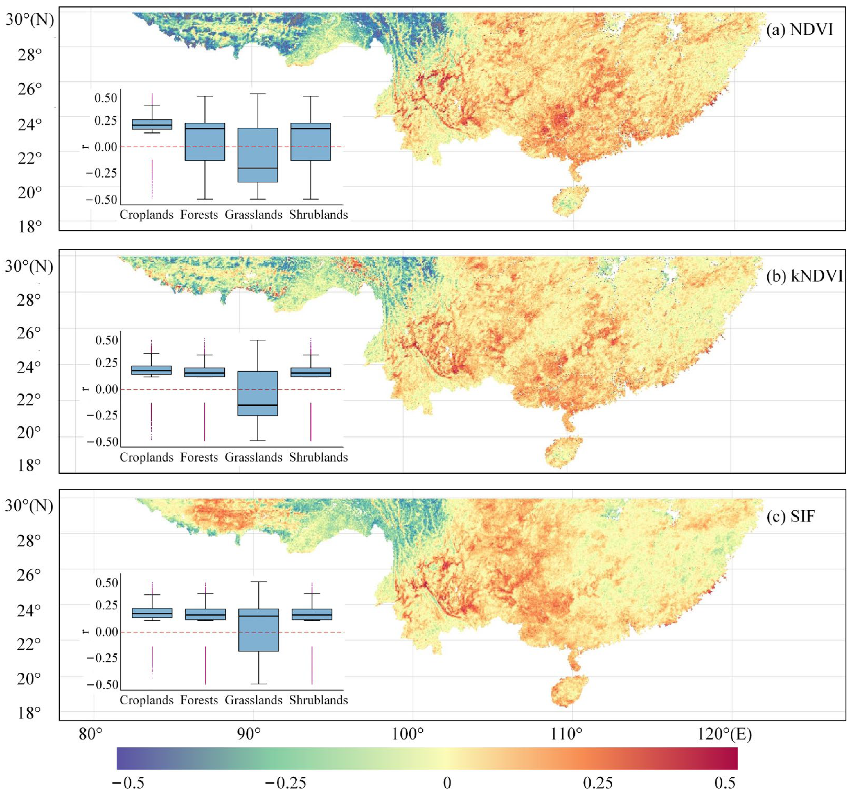
Pearson correlation analysis was performed to explore the relationship among the three vegetation indices with SPEI3 (Figure 2). Our analysis reveals that these three vegetation indices predominantly exhibit positive correlation coefficients with SPEI3. Specifically, the percentages of pixels showing a positive correlation with NDVI-GPP, kNDVI-GPP, and SIF-GPP are 64.29%, 65.61%, and 66.72%, respectively. Notably, these indices demonstrate significant variation in their distribution across different regions and types of vegetation cover. In the Yunnan-Guizhou Plateau, for instance, SIF, NDVI, and kNDVI uniformly respond positively to SPEI3, exhibiting analogous spatial distribution traits. On contrast, in the Himalayan regions characterized by grassland cover, NDVI displays a markedly negative correlation with SPEI3, while kNDVI and SIF predominantly show positive correlations. Furthermore, in the lower altitude areas east of 110°E, particularly in Guangdong and Hunan provinces, the correlation between SIF and SPEI3 is comparatively low, which stands in contrast to the stronger correlation observed with NDVI. When considering the four types of vegetation cover—farmland, forest, shrub, and grassland—the median correlation coefficients between SIF and SPEI3 are positive in all categories, suggesting a robust general relationship between SIF and SPEI3 in these regions. In grassland areas, although NDVI and kNDVI demonstrate a higher degree of response variability, their median values are approximately zero, indicating a neutral overall response.

4.2. SHAP Values of Climatic Factors on Different Vegetation Indices

To detect the effect of climatic changes on vegetation status, we selected six pivotal climatic variables according to their previously established significance in affecting vegetation indices. These variables include VPD, Maximum Temperature (Tmmx), Minimum Temperature (Tmmn), Solar Radiation (Srad), Soil Moisture (SM), and Precipitation (Prec). In this study, we utilized the non-linear lightGBM algorithm to simulate the monthly NDVI, kNDVI, and SIF driven by different factors. The 80% of the time series data in each grid was used for model training, while the remaining 20% data was applied for model accuracy evaluation. The lightGBM model demonstrated satisfactory performance in predicting the NDVI, kNVDI, and SIF for each grid, with R2 scores higher than 0.9 for all grid cells in the test dataset (Table 1).
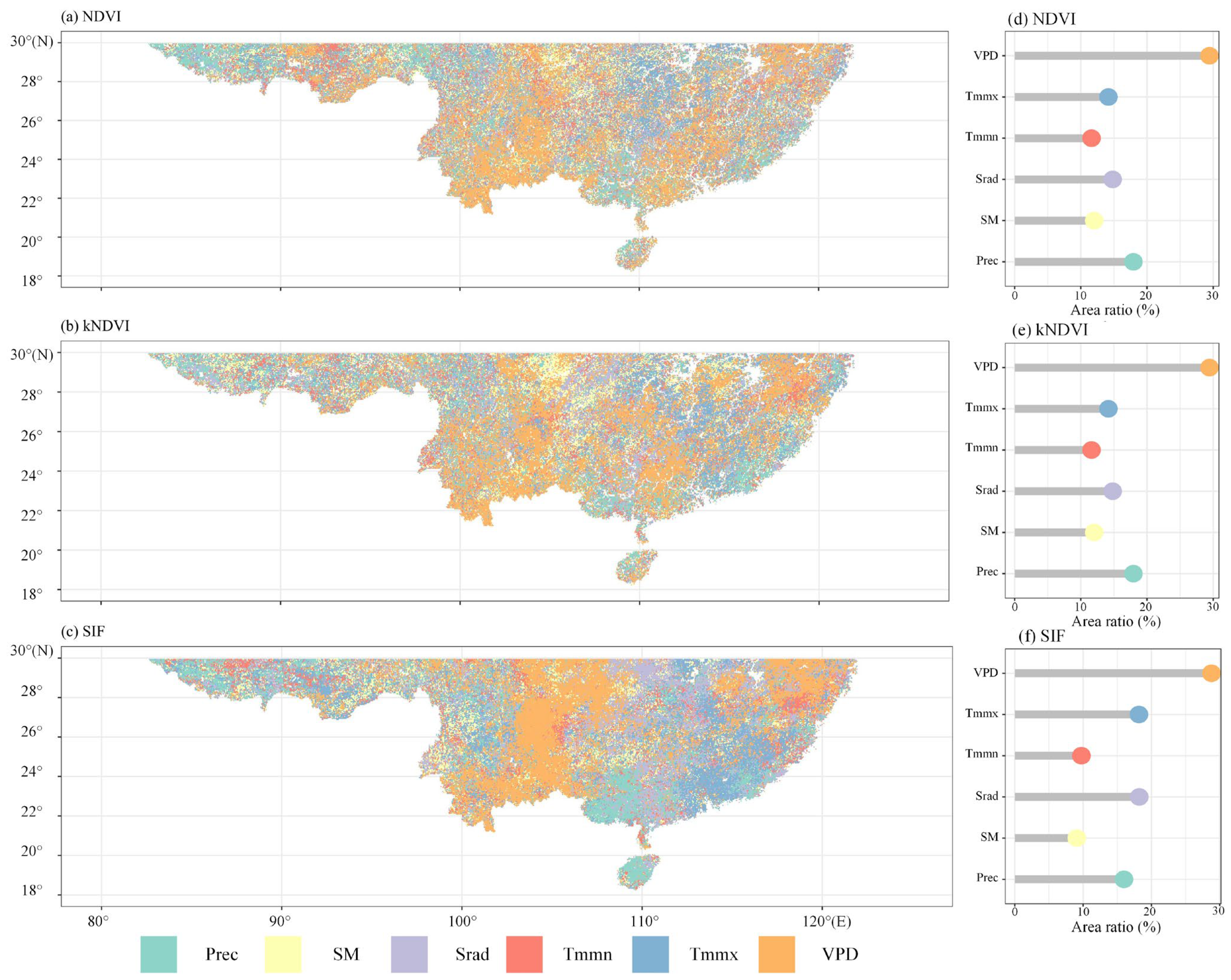
SHAP values were then employed to evaluate the influence of these climatic variables on NDVI, kNDVI, and SIF, as illustrated in Figure 3. The SHAP values serve as a metric for quantifying the contribution of different climatic factors to the accuracy of vegetation index predictions. A higher absolute SHAP Value signifies a more notable contribution of a climatic variable. From Figure 3a–c, we can observe the spatial distribution of the most influential climatic factors for NDVI, kNDVI, and SIF predictions, with key factors identified by their absolute SHAP values. These maps illuminate the spatial variability in the impacts of different climatic variables on vegetation indices. A notable observation is the more dispersed spatial influence on NDVI and kNDVI, compared to a more concentrated impact on SIF, possibly reflecting the differential sensitivities of these indices to climatic variables.
VPD emerges as a predominant factor for all three indices, covering 29.44%, 30.38%, and 28.79% of the area, respectively. This is particularly evident in the central Yunnan-Guizhou Plateau. The findings suggest an acute sensitivity of vegetation in this region to moisture changes, corroborated by the high correlation areas between vegetation indices and SPEI3. For NDVI and kNDVI, precipitation is the second-largest contributing factor, while for SIF, solar radiation (Srad) takes this position, indicating distinct sensitivities of these indices to different climatic variables.
Consistent with the observations in Figure 4, VPD holds the largest impact across all vegetation types, highlighting its key role in vegetation water stress. Interestingly, grasslands exhibit a smaller area influenced by VPD but a relatively greater impact from precipitation, suggesting a higher dependence of grassland vegetation on precipitation compared to other vegetation types. This underscores the diverse responses of different vegetation types to climatic variables.
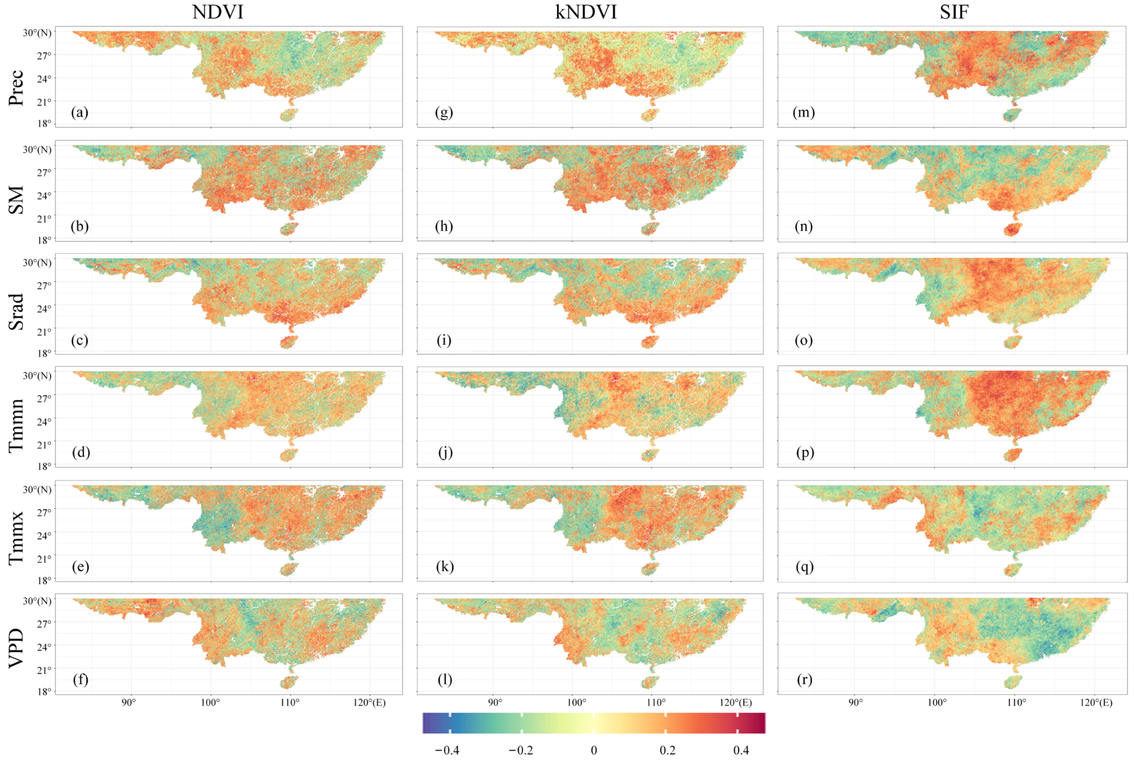
The spatial distribution of SHAP values for NDVI, kNDVI, and SIF concerning the six selected climatic variables were shown in Figure 5. We can observe that, in contrast to NDVI and kNDVI, the SHAP values for climatic factors associated with SIF demonstrate stronger spatial continuity, displaying a distinct spatial pattern. Specifically, SIF exhibits an elevated sensitivity to Precipitation (Prec), Solar Radiation (Srad), and Minimum Temperature (Tmmn). Predominantly, these sensitivities demonstrate as positive SHAP values across most regions, suggesting that these climatic factors actively contribute to the enhancement of SIF values. Conversely, the SHAP values for kNDVI, though bearing spatial resemblance to NDVI, exhibit a more uniform distribution. This is particularly noticeable in regions influenced by Precipitation (Prec) and Maximum Temperature (Tmmx). Such a pattern in kNDVI can potentially be attributed to its ability to reduce data noise and negate the saturation effect inherent in NDVI. This attribute of kNDVI might be contributing to a more continuous and accurate representation of the response to climatic variables. This difference in spatial distribution and sensitivity to climatic factors among NDVI, kNDVI, and SIF, as revealed through SHAP values, underscores the nuanced and complex nature of vegetation index responses to climatic variables. It also highlights the potential of kNDVI in offering a more refined understanding of these relationships, given its enhanced capability to process and reflect climatic influences.

4.3. Response of Different Vegetation Indices to Extreme Drought

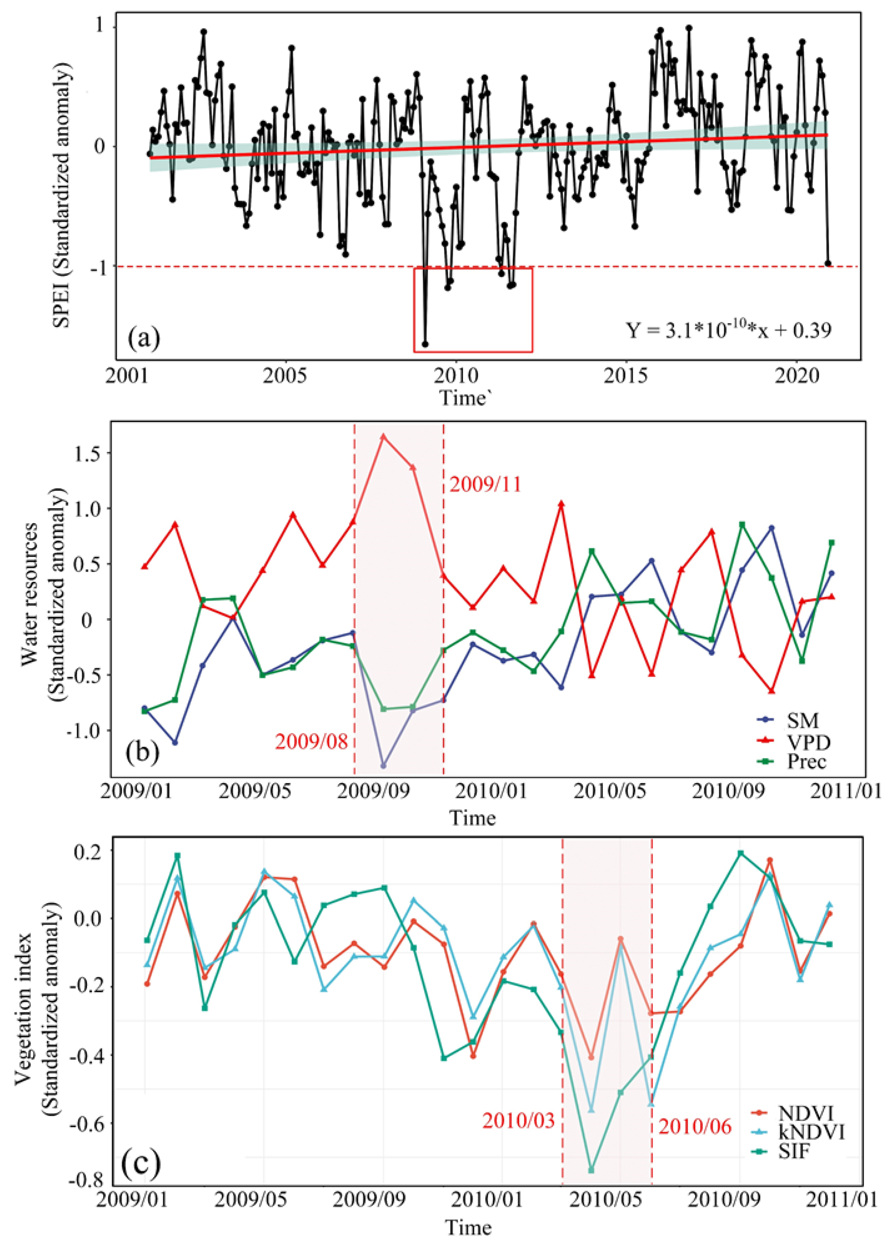
From the time series anomaly of SPEI during 2001–2020 in southern China, we can observe a significant drought event between 2009 and 2010 (Figure 6a). The SPEI anomaly values during this period were below −1, indicating an extreme drought condition in this region. This led to the selection of GPP data from 2009–2010 to examine the response of SIF, NDVI, and kNDVI to this drought event, and to evaluate their efficacy in drought monitoring. between September and October 2009, the Precipitation Anomaly (PrecSA) fell below −0.5, while the Soil Moisture Anomaly (SMSA) and Vapor Pressure Deficit Anomaly (VPDSA) reached below −1.0 and above 1.0, respectively (Figure 6b). These values indicated a severe soil moisture deficiency and high vapor pressure deficit. Following the drought onset, a decline in the three vegetation indices was observed (Figure 6c), with SIF Anomaly (SIFSA) beginning to decrease slightly earlier (January 2010) compared to NDVI Anomaly (NDVISA) and kNDVI Anomaly (kNDVISA), which started in February 2010. All indices reached their lowest anomaly values in April 2010, with SIFSA showing the most significant decline, indicating its higher sensitivity to the extreme drought, followed by kNDVISA, and then NDVISA showing the least decline. To further investigate these three vegetation indices in monitoring vegetation growth response to drought, GPP estimates from three flux tower sites (QYZ, DHS, XSBN) were selected as a benchmark for comparison. The results show that the monthly SIF-GPP relationship at QYZ and XSBN sites was the strongest among all vegetation indices, with R2 values of 0.98 and 0.75, respectively (Figure 7). The NDVI-GPP and kNDVI-GPP relationships at all three sites displayed certain similarities. Notably, at the DHS site, the SIF-GPP relationship (R2 = 0.18) was weaker than the NDVI-GPP and kNDVI-GPP relationships. Conversely, at the XSBN site, the kNDVI-GPP relationship was very weak (R2 = 0.03).
A range of time lags, from direct (0 months) to delayed (up to 4 months) time point, were explored to assess the response of the vegetation index to GPP (Table 2). We calculated the Pearson correlation coefficient between VIs and GPP for each specified lag time by temporarily moving the VIs sequence by the considered lag time. Through this analysis process, we determine the time lag for producing the highest statistically significant correlation coefficients. This lag is considered as the optimal lag, and it contains the time interval when VIs responds most significantly to GPP. Generally, the time-lag relationship of SIF with GPP was shorter than that of NDVI and kNDVI with GPP. At the QYZ site, with a one-month time lag, the relationships of NDVI and kNDVI with GPP reached their maximum values (R2 of 0.8 and 0.81, respectively), whereas the SIF-GPP relationship exhibited no time lag. At the DHS site, no time lag was observed in the relationships between all three vegetation indices and GPP. However, at the XSBN site, the relationships between the vegetation indices and GPP showed different time-lag patterns, with the NDVI-GPP relationship peaking at a two-month lag, the kNDVI-GPP relationship at a three-month lag, and the SIF-GPP relationship at a one-month lag.

4.4. kNDVI Sensitivity with Changing σ

kNDVI has been developed to mitigate the saturation effect observed in the standard NDVI by capturing higher-order differences between the near-infrared and red spectral bands. According to Wang et al. [11], the efficacy of kNDVI hinges on the selection of the kernel function and its hyperparameters. In our study, we opted for the Radial Basis Function (RBF) as the kernel and employed a spatial averaging heuristic method to estimate the optimal kernel parameter σ. Despite these measures, we noted that while kNDVI demonstrated higher spatial consistency with SIF compared to NDVI, and increased sensitivity during drought events, it presented the lowest correlation with site-specific GPP.
This reduced correlation can be attributed to the influence of neighboring pixels in the estimation of the optimal kernel parameter σ, even after accounting for cloud and water body pixels. To address this issue, we recalculated kNDVI employing a temporal averaging heuristic method for estimating the optimal kernel parameter σ, focusing particularly on the 2009–2010 drought period (as illustrated in Figure 8). The outcomes of this recalibration revealed a marked improvement in kNDVI’s (temporal) ability to capture GPP changes, surpassing kNDVI(spatial). At all three examined sites, the correlation between kNDVI (temporal) and GPP was consistently higher than that of kNDVI (spatial). Furthermore, kNDVI (temporal) exhibited a more immediate response in capturing GPP changes induced by drought. It showed no time lag at the QYZ and DHS sites and only a one-month lag at the XSBN site (Table 3). This response time was faster than that of both kNDVI (spatial), and comparable to that of SIF.
These findings highlight the potential of kNDVI for effective monitoring of drought induced GPP changes in vegetation, especially when calculated using temporal heuristic algorithms, which show a higher correlation with GPP than and kNDVI (spatial). The results emphasize the crucial role of selecting the optimal kernel parameter σ to enhance kNDVI’s performance in practical applications.

5. Discussion

5.1. Vegetation Indices Response to Water Stress

The spatial analysis of the correlation between vegetation indices and SPEI3 reveals notable differences in the responses of SIF, NDVI, and kNDVI to moisture stress. These differences are particularly pronounced in the Tibetan Plateau and Guangdong Province. In the Tibetan Plateau, SIF demonstrated a positive correlation with SPEI3. In contrast, the relationships between NDVI-SPEI3 and kNDVI-SPEI3 were less significant, exhibiting no correlation or even negative correlation in certain areas. SPEI3, which accounts for factors such as precipitation and potential evaporation [32], is a critical indicator in assessing the water balance on the surface. The precipitation changes over time are especially crucial in determining the carbon balance of the Tibetan Plateau [33,34]. Our findings suggest that NDVI may not adequately capture the impact of moisture variations on vegetation in this region. This disparity likely arises from the differing sensitivities and mechanisms through which NDVI, kNDVI, and SIF reflect the physiological state of vegetation [35]. NDVI primarily indicates vegetation cover and biomass, while SIF is more directly related to the photosynthetic activity of plants [36,37]. Historical data from 2001 to 2020 show an increase in grassland areas and an upward trend in NDVI in the Tibetan Plateau, which may have partially obscured the response of NDVI to moisture changes [38]. In Guangdong province, earlier studies have identified temperature as a primary factor affecting vegetation growth [39,40]. The saturation effect in NDVI may have contributed to the high positive correlation observed between NDVI and SPEI3. Conversely, kNDVI, with its desaturation property, exhibited a lower correlation with SPEI3, suggesting a more minor different response to moisture conditions. The spatial heterogeneity of vegetation density and growth stages is also an important factor in evaluating the performance of NDVI and kNDVI. In regions with high spatial variability, kNDVI may be better than NDVI because it can better handle this spatial complexity.
The SHAP interpretations for SIF, NDVI and kNDVI all underscore the importance of VPD as a key influencing factor for subtropical terrestrial vegetation growth over southern China. A notable region of high correlation between these three vegetation indices and SPEI3 is the southwestern Yunnan-Guizhou Plateau. This area, characterized by its energy-limited and alpine nature, is highly sensitive to temperature variations, impacting vegetation growth and surface water storage [41]. The diverse landforms of this region, including plateaus, basins, and hills, coupled with unique climatic characteristics and topography, facilitate rapid vegetative responses to changes in moisture conditions. VPD, a primary factor influencing vegetation growth in the Yunnan-Guizhou Plateau, indicates drier air conditions at higher levels, which can enhance water loss through transpiration and stress vegetation [42,43]. Furthermore, SHAP values for SIF reveal that maximum temperature (Tmmx) is a significant influencing factor for vegetation in Guangdong province. In contrast, SHAP interpretations for NDVI indicate that VPD predominantly affects NDVI variations in this region. This finding aligns with the correlation analysis, suggesting that in Guangdong, SIF is less influenced by moisture conditions compared to NDVI, which shows a more significant response to these factors.

5.2. The Outperformance of SIF in Capturing GPP Changes during Drought

Our study highlights the significant advantages of SIF over NDVI and kNDVI in capturing the changes in GPP caused by drought, particularly during the extreme drought event of 2009–2010. SIF exhibited a more sensitive and rapid response to drought stress compared to NDVI and kNDVI. This heightened sensitivity of SIF is attributed to the direct impact of drought conditions on plant photosynthesis. SIF, as a direct measure of photosynthetic activity, can more acutely and promptly reflect changes resulting from environmental stresses like drought [44]. In contrast, NDVI, which primarily represents the overall greenness and biomass of vegetation, can continue to show a relatively healthy vegetative state even under conditions where plants are stressed, and photosynthetic activity is reduced [45]. This disparity arises because NDVI is more a reflection of vegetation cover and biomass, rather than a direct measure of the physiological state of the plants.
Moreover, SIF provides a more precise and timely method for capturing the dynamics of vegetation GPP during drought events. Owing to its direct correlation with the immediate changes in plant photosynthesis, SIF demonstrates a smaller response lag to drought. This characteristic allows it to indicate short-term drought conditions more rapidly. NDVI and kNDVI, on the other hand, exhibit a time lag in reflecting the impacts of drought. This lag is likely due to the time required for significant changes in plant health and biomass to manifest, thus limiting the ability of these indices to provide a real-time indication of drought stress [46].
It is noteworthy that the relationship between SIF and GPP may be affected by the physiological and structural information of SIF, especially under drought conditions [47,48]. Drought stress triggers various physiological responses in plants, such as stomatal closure to reduce water loss through transpiration. This closure reduces the availability of carbon dioxide for photosynthesis, which can lead to a decrease in GPP. Additionally, the changes of canopy structure can influence the amount of light absorbed and emitted by leaves, which will affect both SIF and GPP. It is reported normalizing SIF by the near-infrared radiance of vegetation provides an efficient strategy to normalize SIF to canopy structure [49].
Physiological and structural information of plants under drought conditions can influence the SIF-GPP relationship by affecting photosynthetic efficiency, chlorophyll fluorescence, and other related processes [50,51]. Understanding these relationships is crucial for assessing plant responses to environmental stressors and predicting ecosystem productivity under changing climatic conditions.

5.3. The Performance of kNDVI Is Affected by Hyperparameters

The kNDVI leverages the RBF kernel to enhance the sensitivity and accuracy of vegetation monitoring. A key feature of this approach is the σ parameter, which plays a pivotal role in modulating the index’s sensitivity to vegetation density. For densely vegetated regions, increasing the σ value lowers the kNDVI’s derivative with respect to the NIR and red bands. This adjustment enhances its sensitivity to dense vegetation, enabling the index to capture the nuances of vegetation health that might be missed by traditional indices due to saturation effects. Conversely, reducing the σ value increases kNDVI’s sensitivity to changes in sparsely vegetated areas. This adjustment allows for the detection of subtle vegetation dynamics in environments where traditional vegetation indices may not perform well. The kNDVI effectively captures the spatial characteristics of vegetation drought through the application of a spatial heuristic algorithm. However, it exhibits a low correlation with the GPP of vegetation during drought periods. This correlation with GPP during drought can be enhanced by employing the σ parameter, which is estimated using a temporal heuristic algorithm. This approach underscores the potential for improving kNDVI’s sensitivity to the productivity dynamics of vegetation under drought stress by integrating temporal heuristics. The adjustment of kNDVI’s sensitivity through the σ parameter is underpinned by the RBF kernel’s mathematical properties. The kernel effectively models spatial relationships within spectral data, emphasizing the influence of spectral points that are close in the feature space while reducing the impact of more distant points. This local sensitivity is crucial for adapting the index to specific vegetation conditions, ensuring accurate monitoring across varied ecological landscapes.

6. Conclusions

This research employs the LightGBM-SHAP regression model to conduct a comprehensive examination of the differences between SIF remote sensing data, NDVI, and kNDVI in monitoring vegetation water stress and quantifying the variability of GPP due to drought during the period 2001–2020. The findings reveal that SIF exhibits a higher degree of sensitivity and accuracy in characterizing the anomalous dynamics of GPP during drought periods in comparison to NDVI and kNDVI.
A notable aspect of SIF is its capacity to reflect vegetation response to drought conditions earlier than the other indices, with a time lag of only 0–1 month. This contrasts with NDVI and kNDVI, which demonstrate time lags of 0–3 months and 0–4 months, respectively. This difference is likely attributable to direct correlation of SIF with plant photosynthesis, whereas NDVI primarily indicates overall vegetation greenness and biomass. Moreover, the study underscores that VPD is the predominant climatic factor affecting vegetation changes in regions south of 30°N in China. In terms of kNDVI performance, the research highlights the significant influence of the choice of kernel parameter σ values. Appropriately estimating this parameter can substantially improve the effectiveness of kNDVI in monitoring vegetation drought conditions. Therefore, we suggest that the use of kNDVI should be adapted to the vegetation coverage and growth cycle of the study area to achieve the best results.
Overall, our study validates the advantages of using satellite-based SIF data for monitoring changes in vegetation affected by water resources, particularly in capturing subtropical vegetation GPP changes during droughts. These findings offer valuable guidance in selecting remote sensing indices for timely monitoring and precise assessment of the impacts of hydrological processes on vegetation growth. Furthermore, they pave the way for future research directions, such as exploring the combined impact of additional climatic factors and further refining algorithms and parameter optimization for more accurate monitoring of vegetation status.

Author Contributions

Conceptualization, C.W. and J.W.; methodology, L.L. and Y.Z.; software, C.X.; validation, Y.Z., C.W., L.L., X.L. and X.X.; formal analysis, X.X.; investigation, X.X.; resources, L.L.; data curation, X.X.; writing—original draft preparation, C.W., J.W. and X.X.; writing—review and editing, Y.Z., L.L. and X.L.; visualization, W.T.; supervision, X.X. and Y.Z.; project administration, X.X.; funding acquisition, C.W. and X.X. All authors have read and agreed to the published version of the manuscript.

Funding

This research was funded by Hainan Province Science and Technology Special Fund (Grant No. ZDYF2022GXJS228), Haikou Science and Technology Plan Project (Grant No. 2022-015) and Key Laboratory of Ocean Geomatics, Ministry of Natural Resources China (Grant No. 2021A02).

Data Availability Statement

Data are available within the article.

Conflicts of Interest

The authors declare no conflicts of interest.

References

  1. Martin, E.R. Future Projections of Global Pluvial and Drought Event Characteristics. Geophys. Res. Lett. 2018, 45, 11913–11920. [Google Scholar] [CrossRef]
  2. Slette, I.J.; Post, A.K.; Awad, M.; Even, T.; Punzalan, A.; Williams, S.; Smith, M.D.; Knapp, A.K. How Ecologists Define Drought, and Why We Should Do Better. Glob. Change Biol. 2019, 25, 3193–3200. [Google Scholar] [CrossRef] [PubMed]
  3. Wilhite, D.A.; Glantz, M.H. Understanding: The Drought Phenomenon: The Role of Definitions. Water Int. 1985, 10, 111–120. [Google Scholar] [CrossRef]
  4. Liu, L.; Gudmundsson, L.; Hauser, M.; Qin, D.; Li, S.; Seneviratne, S.I. Soil Moisture Dominates Dryness Stress on Ecosystem Production Globally. Nat. Commun. 2020, 11, 4892. [Google Scholar] [CrossRef] [PubMed]
  5. Liu, X.; Sun, G.; Fu, Z.; Ciais, P.; Feng, X.; Li, J.; Fu, B. Compound Droughts Slow down the Greening of the Earth. Glob. Change Biol. 2023, 29, 3072–3084. [Google Scholar] [CrossRef]
  6. AghaKouchak, A.; Farahmand, A.; Melton, F.S.; Teixeira, J.; Anderson, M.C.; Wardlow, B.D.; Hain, C.R. Remote Sensing of Drought: Progress, Challenges and Opportunities. Rev. Geophys. 2015, 53, 452–480. [Google Scholar] [CrossRef]
  7. Chang, Q.; Zhang, J.; Jiao, W.; Yao, F. A Comparative Analysis of the NDVIg and NDVI3g in Monitoring Vegetation Phenology Changes in the Northern Hemisphere. Geocarto Int. 2018, 33, 1–20. [Google Scholar] [CrossRef]
  8. Ji, L.; Peters, A.J. Assessing Vegetation Response to Drought in the Northern Great Plains Using Vegetation and Drought Indices. Remote Sens. Environ. 2003, 87, 85–98. [Google Scholar] [CrossRef]
  9. Zeng, Y.; Hao, D.; Huete, A.; Dechant, B.; Berry, J.; Chen, J.M.; Joiner, J.; Frankenberg, C.; Bond-Lamberty, B.; Ryu, Y.; et al. Optical Vegetation Indices for Monitoring Terrestrial Ecosystems Globally. Nat. Rev. Earth Environ. 2022, 3, 477–493. [Google Scholar] [CrossRef]
  10. Camps-Valls, G.; Campos-Taberner, M.; Moreno-Martínez, Á.; Walther, S.; Duveiller, G.; Cescatti, A.; Mahecha, M.D.; Muñoz-Marí, J.; García-Haro, F.J.; Guanter, L.; et al. A Unified Vegetation Index for Quantifying the Terrestrial Biosphere. Sci. Adv. 2021, 7, eabc7447. [Google Scholar] [CrossRef]
  11. Wang, Q.; Moreno-Martínez, Á.; Muñoz-Marí, J.; Campos-Taberner, M.; Camps-Valls, G. Estimation of Vegetation Traits with Kernel NDVI. ISPRS J. Photogramm. Remote Sens. 2023, 195, 408–417. [Google Scholar] [CrossRef]
  12. Liu, L.; Yang, X.; Zhou, H.; Liu, S.; Zhou, L.; Li, X.; Yang, J.; Han, X.; Wu, J. Evaluating the Utility of Solar-Induced Chlorophyll Fluorescence for Drought Monitoring by Comparison with NDVI Derived from Wheat Canopy. Sci. Total Environ. 2018, 625, 1208–1217. [Google Scholar] [CrossRef]
  13. Wang, X.; Qiu, B.; Li, W.; Zhang, Q. Impacts of Drought and Heatwave on the Terrestrial Ecosystem in China as Revealed by Satellite Solar-Induced Chlorophyll Fluorescence. Sci. Total Environ. 2019, 693, 133627. [Google Scholar] [CrossRef]
  14. Jiao, W.; Chang, Q.; Wang, L. The Sensitivity of Satellite Solar-Induced Chlorophyll Fluorescence to Meteorological Drought. Earth’s Future 2019, 7, 558–573. [Google Scholar] [CrossRef]
  15. Wang, X.; Biederman, J.A.; Knowles, J.F.; Scott, R.L.; Turner, A.J.; Dannenberg, M.P.; Köhler, P.; Frankenberg, C.; Litvak, M.E.; Flerchinger, G.N.; et al. Satellite Solar-Induced Chlorophyll Fluorescence and near-Infrared Reflectance Capture Complementary Aspects of Dryland Vegetation Productivity Dynamics. Remote Sens. Environ. 2022, 270, 112858. [Google Scholar] [CrossRef]
  16. Liu, Q.; Zhang, F.; Zhao, X. The Superiority of Solar-Induced Chlorophyll Fluorescence Sensitivity over Other Vegetation Indices to Drought. J. Arid Environ. 2022, 204, 104787. [Google Scholar] [CrossRef]
  17. Ma, H.; Cui, T.; Cao, L. Monitoring of Drought Stress in Chinese Forests Based on Satellite Solar-Induced Chlorophyll Fluorescence and Multi-Source Remote Sensing Indices. Remote Sens. 2023, 15, 879. [Google Scholar] [CrossRef]
  18. Shen, Q.; Liu, L.; Zhao, W.; Yang, J.; Han, X.; Tian, F.; Wu, J. Relationship of Surface Soil Moisture with Solar-Induced Chlorophyll Fluorescence and Normalized Difference Vegetation Index in Different Phenological Stages: A Case Study of Northeast China. Environ. Res. Lett. 2021, 16, 024039. [Google Scholar] [CrossRef]
  19. Piao, S.; Nan, H.; Huntingford, C.; Ciais, P.; Friedlingstein, P.; Sitch, S.; Peng, S.; Ahlström, A.; Canadell, J.G.; Cong, N.; et al. Evidence for a Weakening Relationship between Interannual Temperature Variability and Northern Vegetation Activity. Nat. Commun. 2014, 5, 5018. [Google Scholar] [CrossRef] [PubMed]
  20. Cui, L.; Pang, B.; Zhao, G.; Ban, C.; Ren, M.; Peng, D.; Zuo, D.; Zhu, Z. Assessing the Sensitivity of Vegetation Cover to Climate Change in the Yarlung Zangbo River Basin Using Machine Learning Algorithms. Remote Sens. 2022, 14, 1556. [Google Scholar] [CrossRef]
  21. Zhang, J.; Ding, J.; Hou, X.; Wu, P. Quantifying Drought Response Sensitivity and Spatial and Temporal Heterogeneity of Vegetation in Arid and Semi-Arid Regions. Int. J. Remote Sens. 2023, 44, 1665–1683. [Google Scholar] [CrossRef]
  22. Pierrat, Z.A.; Bortnik, J.; Johnson, B.; Barr, A.; Magney, T.; Bowling, D.R.; Parazoo, N.; Frankenberg, C.; Seibt, U.; Stutz, J. Forests for Forests: Combining Vegetation Indices with Solar-Induced Chlorophyll Fluorescence in Random Forest Models Improves Gross Primary Productivity Prediction in the Boreal Forest. Environ. Res. Lett. 2022, 17, 125006. [Google Scholar] [CrossRef]
  23. Ke, G.; Meng, Q.; Finley, T.; Wang, T.; Chen, W.; Ma, W.; Ye, Q.; Liu, T.-Y. LightGBM: A Highly Efficient Gradient Boosting Decision Tree. In Advances in Neural Information Processing Systems; MIT Press: Cambridge, MA, USA, 2017; Volume 30. [Google Scholar]
  24. Lundberg, S.M.; Lee, S.-I. A Unified Approach to Interpreting Model Predictions. In Advances in Neural Information Processing Systems; MIT Press: Cambridge, MA, USA, 2017; Volume 30. [Google Scholar]
  25. Abatzoglou, J.T.; Dobrowski, S.Z.; Parks, S.A.; Hegewisch, K.C. TerraClimate, a High-Resolution Global Dataset of Monthly Climate and Climatic Water Balance from 1958–2015. Sci. Data 2018, 5, 170191. [Google Scholar] [CrossRef] [PubMed]
  26. Martens, B.; Miralles, D.G.; Lievens, H.; van der Schalie, R.; de Jeu, R.A.M.; Fernández-Prieto, D.; Beck, H.E.; Dorigo, W.A.; Verhoest, N.E.C. GLEAM v3: Satellite-Based Land Evaporation and Root-Zone Soil Moisture. Geosci. Model Dev. 2017, 10, 1903–1925. [Google Scholar] [CrossRef]
  27. Miralles, D.G.; Holmes, T.R.H.; De Jeu, R.a.M.; Gash, J.H.; Meesters, A.G.C.A.; Dolman, A.J. Global Land-Surface Evaporation Estimated from Satellite-Based Observations. Hydrol. Earth Syst. Sci. 2011, 15, 453–469. [Google Scholar] [CrossRef]
  28. Li, X.; Huang, W.-R. How Long Should the Pre-Existing Climatic Water Balance Be Considered When Capturing Short-Term Wetness and Dryness over China by Using SPEI? Sci. Total Environ. 2021, 786, 147575. [Google Scholar] [CrossRef]
  29. Liu, Y.; Ding, Z.; Chen, Y.; Yan, F.; Yu, P.; Man, W.; Liu, M.; Li, H.; Tang, X. Restored Vegetation Is More Resistant to Extreme Drought Events than Natural Vegetation in Southwest China. Sci. Total Environ. 2023, 866, 161250. [Google Scholar] [CrossRef]
  30. Shyam, R.; Ayachit, S.S.; Patil, V.; Singh, A. Competitive Analysis of the Top Gradient Boosting Machine Learning Algorithms. In Proceedings of the 2020 2nd International Conference on Advances in Computing, Communication Control and Networking (ICACCCN), Greater Noida, India, 18–19 December 2020; IEEE: Greater Noida, India, 2020; pp. 191–196. [Google Scholar]
  31. Tyralis, H.; Papacharalampous, G.; Doulamis, N.; Doulamis, A. Merging Satellite and Gauge-Measured Precipitation Using LightGBM with an Emphasis on Extreme Quantiles. IEEE J. Sel. Top. Appl. Earth Obs. Remote Sens. 2023, 16, 6969–6979. [Google Scholar] [CrossRef]
  32. Vicente-Serrano, S.M.; Beguería, S.; López-Moreno, J.I. A Multiscalar Drought Index Sensitive to Global Warming: The Standardized Precipitation Evapotranspiration Index. J. Clim. 2010, 23, 1696–1718. [Google Scholar] [CrossRef]
  33. Zhao, J.; Luo, T.; Wei, H.; Deng, Z.; Li, X.; Li, R.; Tang, Y. Increased Precipitation Offsets the Negative Effect of Warming on Plant Biomass and Ecosystem Respiration in a Tibetan Alpine Steppe. Agric. For. Meteorol. 2019, 279, 107761. [Google Scholar] [CrossRef]
  34. Han, P.; Lin, X.; Zhang, W.; Wang, G.; Wang, Y. Projected Changes of Alpine Grassland Carbon Dynamics in Response to Climate Change and Elevated CO2 Concentrations under Representative Concentration Pathways (RCP) Scenarios. PLoS ONE 2019, 14, e0215261. [Google Scholar] [CrossRef] [PubMed]
  35. Jeong, S.-J.; Schimel, D.; Frankenberg, C.; Drewry, D.T.; Fisher, J.B.; Verma, M.; Berry, J.A.; Lee, J.-E.; Joiner, J. Application of Satellite Solar-Induced Chlorophyll Fluorescence to Understanding Large-Scale Variations in Vegetation Phenology and Function over Northern High Latitude Forests. Remote Sens. Environ. 2017, 190, 178–187. [Google Scholar] [CrossRef]
  36. Lu, X.; Liu, Z.; Zhou, Y.; Liu, Y.; An, S.; Tang, J. Comparison of Phenology Estimated from Reflectance-Based Indices and Solar-Induced Chlorophyll Fluorescence (SIF) Observations in a Temperate Forest Using GPP-Based Phenology as the Standard. Remote Sens. 2018, 10, 932. [Google Scholar] [CrossRef]
  37. Wang, X.; Dannenberg, M.P.; Yan, D.; Jones, M.O.; Kimball, J.S.; Moore, D.J.P.; Van Leeuwen, W.J.D.; Didan, K.; Smith, W.K. Globally Consistent Patterns of Asynchrony in Vegetation Phenology Derived from Optical, Microwave, and Fluorescence Satellite Data. JGR Biogeosci. 2020, 125, e2020JG005732. [Google Scholar] [CrossRef]
  38. Li, Y.; Gong, J.; Zhang, Y.; Gao, B. NDVI-Based Greening of Alpine Steppe and Its Relationships with Climatic Change and Grazing Intensity in the Southwestern Tibetan Plateau. Land 2022, 11, 975. [Google Scholar] [CrossRef]
  39. Wu, Y.; Tang, G.; Gu, H.; Liu, Y.; Yang, M.; Sun, L. The Variation of Vegetation Greenness and Underlying Mechanisms in Guangdong Province of China during 2001–2013 Based on MODIS Data. Sci. Total Environ. 2019, 653, 536–546. [Google Scholar] [CrossRef] [PubMed]
  40. He, G.; Li, Z. Asymmetry of Daytime and Nighttime Warming in Typical Climatic Zones along the Eastern Coast of China and Its Influence on Vegetation Activities. Remote Sens. 2020, 12, 3604. [Google Scholar] [CrossRef]
  41. Zhou, Q.; Luo, Y.; Zhou, X.; Cai, M.; Zhao, C. Response of Vegetation to Water Balance Conditions at Different Time Scales across the Karst Area of Southwestern China—A Remote Sensing Approach. Sci. Total Environ. 2018, 645, 460–470. [Google Scholar] [CrossRef] [PubMed]
  42. Tian, Y.; Bai, X.; Wang, S.; Qin, L.; Li, Y. Spatial-Temporal Changes of Vegetation Cover in Guizhou Province, Southern China. Chin. Geogr. Sci. 2017, 27, 25–38. [Google Scholar] [CrossRef]
  43. Zhang, X.; Yue, Y.; Tong, X.; Wang, K.; Qi, X.; Deng, C.; Brandt, M. Eco-Engineering Controls Vegetation Trends in Southwest China Karst. Sci. Total Environ. 2021, 770, 145160. [Google Scholar] [CrossRef]
  44. Zhang, Y.; Joiner, J.; Gentine, P.; Zhou, S. Reduced Solar-induced Chlorophyll Fluorescence from GOME -2 during Amazon Drought Caused by Dataset Artifacts. Glob. Change Biol. 2018, 24, 2229–2230. [Google Scholar] [CrossRef]
  45. Kim, J.Y.; Glenn, D.M. Multi-Modal Sensor System for Plant Water Stress Assessment. Comput. Electron. Agric. 2017, 141, 27–34. [Google Scholar] [CrossRef]
  46. Chen, S.; Huang, Y.; Wang, G. Detecting Drought-Induced GPP Spatiotemporal Variabilities with Sun-Induced Chlorophyll Fluorescence during the 2009/2010 Droughts in China. Ecol. Indic. 2021, 121, 107092. [Google Scholar] [CrossRef]
  47. Xu, S.; Atherton, J.; Riikonen, A.; Zhang, C.; Oivukkamäki, J.; MacArthur, A.; Honkavaara, E.; Hakala, T.; Koivumäki, N.; Liu, Z.; et al. Structural and photosynthetic dynamics mediate the response of SIF to water stress in a potato crop. Remote Sens. Environ. 2021, 263, 112555. [Google Scholar] [CrossRef]
  48. Kimm, H.; Guan, K.; Jiang, C.; Miao, G.; Wu, G.; Suyker, A.E.; Ainsworth, E.A.; Bernacchi, C.J.; Montes, C.M.; Berry, J.A.; et al. A physiological signal derived from sun-induced chlorophyll fluorescence quantifies crop physiological response to environmental stresses in the US Corn Belt. Environ. Res. Lett. 2021, 16, 124051. [Google Scholar] [CrossRef]
  49. Zeng, Y.; Chen, M.; Hao, D.; Damm, A.; Badgley, G.; Rascher, U.; Johnson, J.E.; Dechant, B.; Siegmann, B.; Ryu, Y.; et al. Combining near-infrared radiance of vegetation and fluorescence spectroscopy to detect effects of abiotic changes and stresses. Remote Sens. Environ. 2022, 270, 112856. [Google Scholar] [CrossRef]
  50. Wieneke, S.; Burkart, A.; Cendrero-Mateo, M.; Julitta, T.; Rossini, M.; Schickling, A.; Schmidt, M.; Rascher, U. Linking photosynthesis and sun-induced fluorescence at sub-daily to seasonal scales. Remote Sens. Environ. 2018, 219, 247–258. [Google Scholar] [CrossRef]
  51. Wu, L.; Zhang, X.; Rossini, M.; Wu, Y.; Zhang, Z.; Zhang, Y. Physiological dynamics dominate the response of canopy far-red solar-induced fluorescence to herbicide treatment. Agric. For. Meteorol. 2022, 323, 109063. [Google Scholar] [CrossRef]
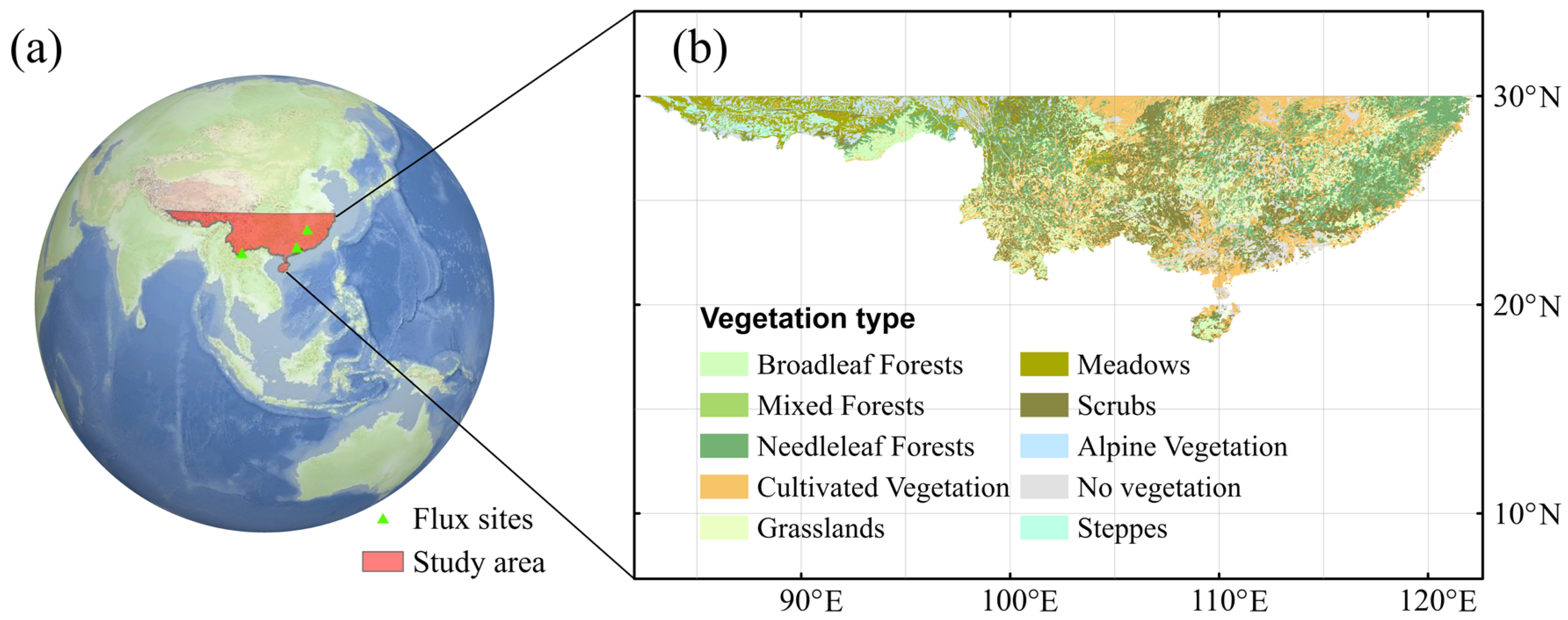
Figure 1. Map of study area (a), (red polygon) and the corresponding vegetation types (b).
Remotesensing 16 01735 g001
Figure 2. Correlations between vegetation indicators and SPEI3.
Remotesensing 16 01735 g002
Figure 3. Spatial distribution of the maximum SHAP value environmental factors to NDVI (a), KNDVI (b), and SIF (c) from 2001 to 2020 and the proportion of each factor (df).
Remotesensing 16 01735 g003
Figure 4. The proportion of the maximum SHAP value factor to NDVI (a), kNDVI (b), and SIF (c) under different vegetation types during 2001–2020.
Remotesensing 16 01735 g004
Figure 5. Spatial distribution of the SHAP value of environmental factors to NDVI (af), KNDVI (gl), and SIF (mr) from 2001 to 2020.
Remotesensing 16 01735 g005
Figure 6. Extreme drought in Southern China during 2001–2020 (a), changes of different water resources during extreme drought (b), and comparison of responses of vegetation index to extreme drought (c).
Remotesensing 16 01735 g006
Figure 7. Relationships between tower flux site GPP and satellite derived NDVI, kNDVI, and SIF.
Remotesensing 16 01735 g007
Figure 8. Relationships between tower flux site GPP and kNDVI (temporal), kNDVI (spatial).
Remotesensing 16 01735 g008
Table 1. Mean Absolute Error (MAE), Root Mean Squared Error (RMSE), and the coefficient of determination (R-squared) of lightGBM model.
ModelMAERMSER2
NDVI0.13520.18950.9674
kNDVI0.13470.18860.9672
SIF0.12110.17110.9703
Table 2. Coefficient of determination (R2) for correlation analysis between monthly GPP and NDVI, kNDVI and SIF at different time lags. Red color indicates a significance test pass (p < 0.05), with darker shades representing a larger lag coefficient of determination.
SitesVIsR2 Values between VIs and GPP at Different Time Lags (Months)
01234
QYZNDVI0.790.80.40.050.07
kNDVI0.720.810.530.120.02
SIF0.920.630.3700.24
DHSNDVI0.380.210.0300.12
kNDVI0.370.190.080.10.03
SIF0.1800.070.030
XSBNNDVI0.350.50.590.410.1
kNDVI0.030.070.370.610.48
SIF0.750.780.420.050
Table 3. R2 values resultant from correlations between monthly GPP and monthly kNDVI (temporal) at different time lags.
SitesR2 Values between kNDVI (Temporal) and GPP at Different Time Lags (Months)
01234
QYZ0.830.820.470.040.06
DHS0.580.330.1800.35
XSBN0.380.630.60.20.03
Disclaimer/Publisher’s Note: The statements, opinions and data contained in all publications are solely those of the individual author(s) and contributor(s) and not of MDPI and/or the editor(s). MDPI and/or the editor(s) disclaim responsibility for any injury to people or property resulting from any ideas, methods, instructions or products referred to in the content.