Abstract
This article focuses on developing models that estimate suspended sediment concentrations (SSCs) for the Lower Brazos River, Texas, U.S. Historical samples of SSCs from gauge stations and satellite imagery from Landsat Missions and Sentinel Mission 2 were utilized to develop models to estimate SSCs for the Lower Brazos River. The models used in this study to accomplish this goal include support vector machines (SVMs), artificial neural networks (ANNs), extreme learning machines (ELMs), and exponential relationships. In addition, flow measurements were used to develop rating curves to estimate SSCs for the Brazos River as a baseline comparison of the models that used satellite imagery to estimate SSCs. The models were evaluated using a Taylor Diagram analysis on the test data set developed for the Brazos River data. Fifteen of the models developed using satellite imagery as inputs performed with a coefficient of determination R2 above 0.69, with the three best performing models having an R2 of 0.83 to 0.85. One of the best performing models was then utilized to estimate the SSCs before, during, and after Hurricane Harvey to evaluate the impact of this storm on the sediment dynamics along the Lower Brazos River and the model’s ability to estimate SSCs.
1. Introduction
Suspended sediment transport in river basins is important for many water management planning activities, including the estimation of the useful life of reservoirs, the evaluation of land use impacts, and quantifying sediment-associated nutrient and contaminant amounts. In general, increased amounts of suspended sediment can lead to increased amounts of contaminants in water because many contaminants can be attached to suspended sediment particles or are suspended particles. This increased level of contamination can affect treatment processes. Also, increased suspended sediment can lead to increased sedimentation within reservoirs that reduces their overall capacity, which could cause future water capacity shortages. Furthermore, increased suspended sediment can adversely affect native aquatic life. Thus, it can be very valuable to accurately estimate SSCs in waterbodies.
Currently, the traditional way to measure suspended sediment effectively and reliably is by collecting field samples in the river body. This method is very time-consuming and can be extremely dangerous for field staff following severe flooding events [1]. These field samples also only provide a point value of suspended sediment within the waterbody at the instant the sample was taken.
These field sediment samples, specifically SSCs, are usually used along with flow measurements taken at the same time as the field sediment samples to develop a load rating curve that estimates the SSC or sediment load. This method of estimating the SSC or sediment load relies on the general assumption that increasing flows lead to increased sediment being conveyed by the river. However, this assumption may not always be true in all rivers due to the complexities of the sediment transport processes that result from the soil properties and land use/land cover of the river’s watershed, and in-river processes that result in complex colloids and bed material interactions [2,3,4,5,6]. These complexities can result in peak SSC occurring before or after peak flows on the rising or receding limb of a flow hydrograph during a storm event.
Efforts have been made in recent years to use less labor-intensive methods that do not rely on flow to estimate SSC, including use of satellite imagery data, specifically surface reflectance data. Satellite imagery data can provide a spatial measure of suspended sediment that field data cannot produce without significant effort [7]. It can also potentially provide a more continuous record than field measurements depending on the cloud cover on the date the image was captured and the return frequency of the satellite [8]. Typically, the timing of satellite imagery data is at best daily to every other day with newer technologies that are publicly available.
In contrast to the benefits mentioned above, the use of satellite imagery data to estimate SSCs comes with its challenges because it is an optical measure. Researchers have noted that factors associated with satellite imagery, such as sunglint, cloud cover, boat navigations, the frequency of image collection, and the presence of organic materials such as chlorophyll- in water [7,8], affect its use when estimating SSCs. Many researchers have used simple filters based on the satellite imagery data measurements or other field measurements (in the case of the presence of organic material) to reduce the effects of these factors associated with satellite imagery.
In addition to the limitations mentioned above, using satellite imagery data to estimate SSCs faces many of the same challenges faced by researchers that have used turbidity to estimate SSCs. These challenges include the effect of the particle size and color of the suspended sediment on the optical reflectance values and the importance of collecting SSC samples during storm events [9,10,11,12]. Both the particle size and color of the suspended sediment are region-specific and can vary over time within a watershed depending on seasonality and changing development patterns. These factors can make any relationship developed to estimate SSCs using satellite imagery vary over time and limit the model’s ability to be used in other regions. Furthermore, if SSC samples have not been collected during major storm events, the largest SSC that the river body could have seen would be missing, thus limiting the applicable range of a model to estimate SSCs using satellite imagery.
To counteract some of the challenges and complexities that are present in models that estimate SSCs using satellite imagery, researchers have begun to use more complex modeling algorithms to accurately predict the relationship between satellite imagery surface reflectance and SSCs [1,7,8]. Researchers have used a wide range of machine learning models, including, but not limited to, ANNs, SVMs, decision trees, genetic algorithms, adaptive neuro-fuzzy inference systems, and ELMs [13,14]. Specifically, ANNs have been extensively used, and ELMs have shown superior performance compared to other machine learning models.
In addition to implementing complex models, some researchers have also begun to use more physics-based modeling techniques to estimate measurements in waterbodies. A physics-based approach is most common in waterbodies when optical measurements are utilized to estimate water depth by creating data collection procedures to focus on bottom reflectance and column reflectance measurements and developed models based on the Beer–Lambert Law [15,16]. It is also common to use band ratios in the developed models [17]. The researchers who use band ratios theorize that band ratios capture the underlying physical properties of how the water absorbs different wavelength frequencies of light, allowing the model to perform better than models that do not incorporate band ratios.
In this study, the goal was to develop a model that estimates SSC through satellite imagery data for the Lower Brazos River near the Gulf of Mexico, Texas, U.S., using publicly available data. This area is particularly valuable in developing such an SSC estimator because the understanding of the sediment dynamics of the Brazos River has become an environmental concern for local officials and communities that are trying to mitigate the river’s impact on the nearby San Bernard River. This primary goal focused on developing machine learning models and an exponential model with physics-based roots that used surface reflectance values from both Landsat and Sentinel Mission 2 satellite imagery data to estimate SSCs. This study also had the secondary goal of evaluating a top performing model during a notable storm event to determine its ability to estimate SSCs. Specifically, one of the developed models was used to estimate SSCs in the Lower Brazos River before, during, and after Hurricane Harvey.
2. Materials and Methods
2.1. Study Area
The focus of this study was to estimate the SSCs within the Lower Brazos River near the outfall to the Gulf of Mexico. The Brazos River watershed is one of the largest in Texas, with a total surface area of approximately 44,620 square miles, originating in New Mexico and terminating in Brazoria County near Freeport, Texas. The river conveys a large sediment load that has led to net deposition in the Gulf of Mexico near the mouth of the river [18]. This has led to issues with the nearby San Bernard River mouth closing and requiring frequent dredging. The San Bernard River is directly south of the Brazos River watershed and directly north of the Colorado River watershed. This study builds on the work conducted by others in the Brazos River [19] to help develop an accurate SSC estimator that will help future researchers and engineers evaluate the sediment characteristics of the Brazos River to combat the issues it is causing in the San Bernard River. The specific area for which the model was developed, along with the United States Geological Survey (USGS) and Texas Commission on Environmental Quality (TCEQ) sampling site locations whose data were used, are illustrated in Figure 1.
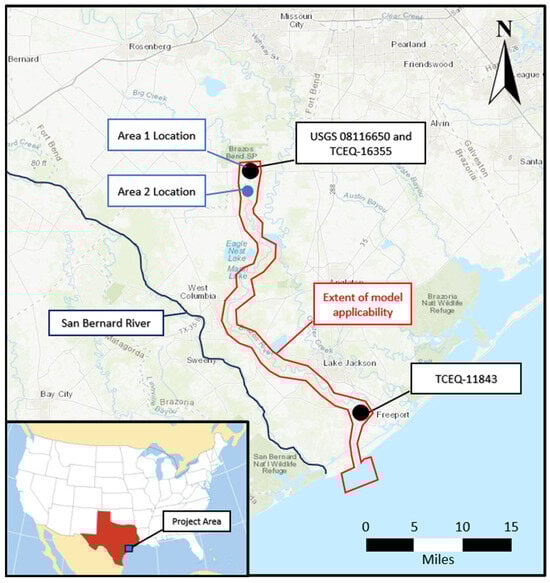
Figure 1.
Map of the study area showing extents of model development, the USGS and TCEQ sampling sites whose data were used for model development, and the two upstream areas used to evaluate the model’s performance during the case study.
2.2. SSC Data
Two sampling locations with publicly available SSC data from the National Water Quality Monitoring Council (NWQMC) and data collected by previous researchers along the Brazos River were used for this study. These sampling locations included three unique numbered gauging locations owned and maintained by two different agencies. The northernmost location near Rosharon, TX, has two gauges operated by the USGS and TCEQ (USGS 08116650 and TCEQ-16355), while the southernmost location near Freeport, TX, has one TCEQ gauging location (TCEQ-11843). The locations of these gauges and a summary of the SSC data from these gauges used in this study are presented in Figure 1 and Figure 2, respectively. Table 1 documents some important summary statistics for each of the gauging locations. Six of the data points shown for the northernmost gauging location near Rosharon, TX (USGS 08116650), were collected during a past study conducted along the Brazos River [19]. Sampling methods by the USGS were either suspended sediment concentration tests or total suspended sediment tests, while the TCEQ methods were exclusively total suspended sediment tests [20]. Both agencies used either the equal-width-increment or the equal-discharge-increment method for sampling and followed the American Society for Testing and Materials standards [19]. The past study used the Federal Interagency Sedimentation Project depth-integrated sampler and the equal-width-increment method for SSC samples [19].
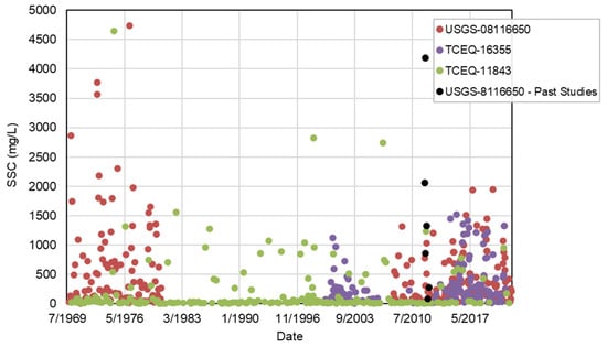
Figure 2.
SSC data for the Brazos River used for this study.

Table 1.
Summary statistics of SSC data used in this study.
2.3. Flow Data
Flow data from the USGS 08116650 were used for this study to compare models developed using satellite data to the standard SSC estimation method of a load rating curve. In practice, a load rating curve is either used to estimate SSCs or sediment load. For this study, only the SSC method was investigated to compare models developed using satellite data. The average daily flow records at the USGS 08116650 were linked to the SSC data collected on the same day, resulting in a total of 470 pairs of flow and sediment data. Figure 3 shows the data pairs at the USGS 08116650 for flow and sediment. Log-scales were used for both the x and y axes because this is common practice for the load rating curve method. The SSC data shown in Figure 3 include samples collected at TCEQ-16355, since they are approximately the same location.
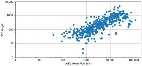
Figure 3.
Daily mean flow vs. SSC for the Brazos River at USGS 08116650 using data from USGS 08116650 and TCEQ-16355.
2.4. Satellite Data and Preparation
Two sources of publicly available optical image satellite data were used for this study: the Landsat and Sentinel satellite missions. Landsat satellite data are collected, processed, and provided by the USGS, with satellite data going back to July 1972 and nine total missions. The Landsat images for Missions 1–3 were collected at a 60 m (196.8 ft) resolution, while the images for Missions 4 and onwards were/are collected at a 30 m (98.4 ft) resolution. Because of the narrow width of the Brazos River at the upstream sample location near Rosharon, TX (an approximately 170 ft wide channel based on aerial imagery), Landsat Missions 1–3 were not used for this study.
Sentinel satellite data are collected, processed, and provided by the European Space Agency (ESA). There are six Sentinel Missions that each collect specific data such as air quality tracers or optical imagery. Sentinel Mission 2 is the mission that collects optical imagery and was used for this study. Two satellites (A and B) are actively measuring optical imagery for Sentinel Mission 2. Satellite A was launched in 2016, while satellite B was launched in 2018. The resolution of data collected for Sentinel Mission 2 are either 10 m, 20 m, or 60 m. As mentioned above, narrow river widths at the upstream sample location near Rosharon, TX, prevent the use of images that are 60 m in resolution from this data source.
Figure 4 summarizes the different bands of data collected by all the satellites used in this study (Landsat Missions 4–9 and Sentinel Mission 2). Landsat Mission 9 collected the same bands as Landsat Mission 8. Likewise, Landsat Missions 4 and 5 collected the same bands as Landsat Mission 7. As shown in Figure 4, many of the bands were collected over the exact same or a very similar range of wavelengths across all missions used in this study. The following bands were used from the different missions for this study.
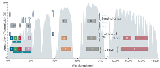
Figure 4.
Comparison of Landsat Mission and Sentinel Mission 2 bands collected for this study [21]. The different bands depicted in the figure are the numberings used for the specific mission, and the width of the band’s shape represents the range of the wavelength of light collected for the band. For example, Band 1 for Landsat Mission 7 (L7 ETM+) is light of wavelength 450–520 nm.
- Landsat Missions 4–7: Bands 1–5 and 7.
- Landsat Missions 8–9: Bands 2–7.
- Sentinel Mission 2: Bands 2–4, 8, and 11–12.
For the Sentinel Mission 2 bands used in this study, Bands 2–4 and 8 have a resolution of 10 m, and Bands 11–12 have a resolution of 20 m. Bands with similar ranges of wavelength of light collected by the different satellite missions were assumed to represent the same values and were grouped in the same category for this study. For example, Band 4 from Landsat Missions 4–7, Band 5 from Landsat Missions 8–9, and Band 8 from Sentinel Mission 2 were labeled as NIR bands. The band groups used for this study are shown in Table 2.
Table 2.
Band groups from satellite missions used in this study.
For this study, Level 2 data products were used because this level of product is the highest for both Landsat and Sentinel images that is provided. More importantly, this level of product is a measure of surface reflectance values that are atmospherically corrected by processing algorithms developed by the space agencies to correct for potential errors in satellite measurements, such as the sun angle and angle of instrument measurement. Landsat Missions provide Level 2 processed data for all missions used in this study (Missions 4–9) and have valid reflectance value ranges from 7273 to 43,636. Sentinel Mission 2 data only started providing Level 2 products following December 2018. For images before December 2018 for Sentinel Mission 2 data, ESA-provided data-processing tools were used to create Level 2 products from the Level 1C data collected. Sentinel Mission 2 data have valid reflectance value ranges from 1 to 10,000. A total of 1312 Landsat images were collected using EarthExplorer tools provided by the USGS, and a total of 912 Sentinel Mission 2 images were collected using Sentinel Application Programming Interface (API) calls.
Satellite Data Preparation
Buffer areas near the sampling locations used in this study were created to determine a representative pixel value for the sampling sites. The average of the pixel values in the buffer area was used for this representative value. Buffer areas were created upstream of the sampling locations to incorporate pixels that only contained water based on a combination of aerial imagery and quality pixel values provided by the space agencies. It was observed that the stream path of the Brazos River did not change at the sample locations in this study over the period of satellite data collected based on the historical aerial images and quality pixels. Thus, static buffer areas were created for this study. The buffer areas were created based on the 30 m by 30 m pixels from Landsat and are shown in Figure 5. These buffer areas did not require any updates to be used for Sentinel Mission 2 Bands 11–12 that have a resolution of 20 m by 20 m, because they were observed to not capture any non-water 20 m by 20 m pixels.
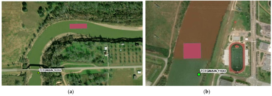
Figure 5.
Buffer areas (red polygons) used to generate a representative pixel value for sample site locations in this study. Panel (a) shows the 90 m by 30 m buffer used at the upstream sampling location near Rosharon, TX on the Brazos River; panel (b) shows the 90 m by 90 m buffer at the downstream sampling location near Freeport, TX, on the Brazos River.
The quality pixels were used to remove average pixel values from the buffer areas to prevent the interference of clouds with surface reflectance values. More specifically, any of the quality pixels with values that indicated any cloud cover, saturation, or snow/ice in the buffer area resulted in the removal of that scene for use at that sample location. It was observed that quality pixel values were not always labeled as water pixels and could have been labeled bare soils/land, cloud shadow, or dark areas. It was hypothesized this occurred because of the general nature of the quality labeling algorithms used by the USGS and ESA. Thus, scenes with these non-water labels were not removed for this study.
The satellite data that were collected for this study were linked to the closest SSC sample data by the date of their acquisition. This means that satellite images could be linked to SSC samples that were obtained before, on the same day as, or after the date of acquisition of the satellite images. For this study, only pairs of satellite and SSC data with up to a 3-day difference in their acquisition dates were used to be consistent with the maximum day difference used by previous researchers. The valid data range for the Landsat Missions and Sentinel Mission 2 were used to convert raw surface reflectance values to percentages to allow the use of both sources for SSC estimation.
Daily mean flow data at the USGS 08116650 (near Rosharon, TX) were used to evaluate whether a large change in flow occurred between the dates of satellite image and SSC sample acquisition to remove pairs of satellite imagery and SSC data that were not collected on the same day. This was carried out because SSC is likely to change the most during rainfall/flood events, and satellite images not taken on the same day during these events would potentially miss these changes. Figure 6 illustrates SSC, daily mean flow, and the day lag between satellite image and SSC acquisition dates, where negative values mean the satellite image was taken after the SSC sample was acquired. As shown in this figure, the satellite images for sample points on 1/28/12 and 1/30/12 were taken 1 and 3 days before SSC sample acquisition just before a major flood event. Thus, both sample points on 1/28/12 and 1/30/12 were removed from the dataset. In addition to removing points based on proximity to flood events, any satellite images that were linked to multiple suspended sediment concentration samples were only retained as a data pair for the closest sample date. An example of this data exclusion is shown in Figure 6 for the sample points on 1/10/12 and 1/11/12, where the data pair for the sample on 1/10/12 was excluded from the final data set.
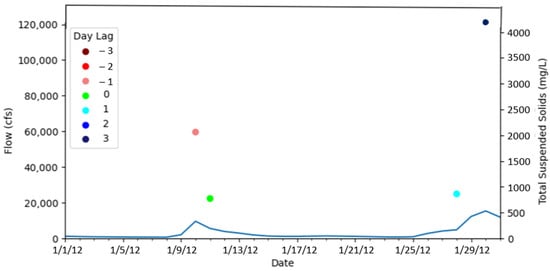
Figure 6.
Example of flow, SSC, and acquisition lag filtering analysis used for this study.
This same methodology was used for SSC samples collected at the TCEQ-11843 station. Since no flow data were available near this sampling site, it was assumed that the upstream USGS gauge could be a good indication of flood events downstream.
The resulting relationships between the six satellite bands and SSC following this removal procedure are shown in Figure 7. This data refinement resulted in a total of 210 (138 for Landsat Missions and 72 for Sentinel Mission 2) satellite and SSC sample pairs for the Brazos River that were used for this study.
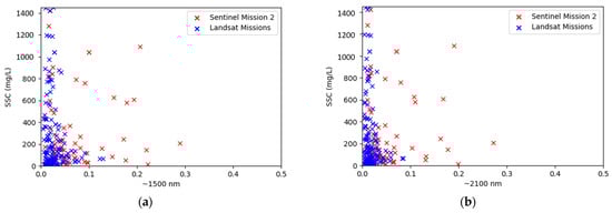
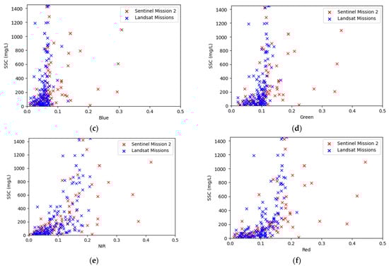
Figure 7.
Final filtered and processed normalized surface reflectance values and SSC sample data used for this study with (a) ~1500 nm band; (b) ~2100 nm band; (c) blue band; (d) green band; (e) NIR band; (f) red band.
2.5. Modeling Techniques
This section provides technical details of the modeling techniques used in this study, including the rating curve, ANN, SVM, ELM, and the developed exponential relationship.
2.5.1. Rating Curve
As mentioned previously, the rating curve method is a very common approach to estimating SSCs that uses flow measurements. Equation (1) shows the typical rating curve used to estimate SSCs:
where and are coefficients that are calibrated for a site, SSC (mg/L) is the suspended sediment concentration, and Q (cfs) is the stream flow [19]. In this formulation, the unit of coefficient is mg/L × (cfs)−b.
In practice, it is more common to use a rating curve method to estimate sediment load, but this was not pursued in this study to provide an easier comparison to the other models developed.
2.5.2. ANN
ANNs are composed of nodes that use outputs from nodes in previous layers of the neural network, weighted by values that are calibrated, to produce the desired output. Each node in the neural network uses Equation (2), where (x) is called the activation function, W is a matrix of weights, z is a vector of either outputs from the previous layer or a matrix of the inputs, and b is a vector of coefficients [22,23].
Three activation functions, the sigmoid function, the hyperbolic tangent (TanH) function, and the rectified linear unit (ReLU) function, were used as hyperparameters in this study. All three activation functions are provided in Equations (3)–(5).
In addition to the activation function, the learning rate, alpha, and momentum hyperparameters were tuned in this study. Alpha in this context is the term that controls the L2 regularization. Stochastic gradient descent was used for training the ANNs in this study [22,23].
2.5.3. SVM
SVMs were originally created for classification applications. The original version of the algorithm creates a linear decision boundary using Equation (6). In this equation, W is a matrix of weights, x is a matrix of inputs, and b is a vector of coefficients [22,23].
The original form of the SVM has been modified in recent years to allow it to estimate numerical values and use non-linear decision boundary functions, and to allow for minimization of the overfitting of the model [22,23]. Equation (7) shows the SVM cost function used in this study.
where C determines the tradeoff between increasing the size of the decision boundary and ensuring each data point lies on the correct side of the decision boundary by controlling the Euclidean norm of the weights, is a way to simplify the constraints of if and if and produces a value of 1 when the constraints are met and 0 otherwise, and φ is the kernel function [22,23].
2.5.4. ELM
An ELM has a similar structure to an ANN as it has an input layer, a hidden layer, and an output layer. Unlike an ANN, an ELM uses an optimization approach to solve for weights. The cost function used for an ELM is shown in Equation (8), where x is the input data, y is the actual output, w is the weight vector and b is the bias vector of the hidden node j, and (x) is a nonlinear activation function [24]. The output weight vector is denoted by and links the hidden node and the output node.
When the above cost function is minimized, it is set equal to zero. In this case, Equation (8) can be rewritten as Equation (9). In this simplified form, T is a matrix of true outputs, H is a matrix of the hidden layer where each column is a node, and is a matrix of the output weights [24].
In this algorithm, the weights and bias values in the hidden layer are initially assigned randomly and are unadjusted throughout the training process. Only output weights are adjusted through the training process. Thus, the above equation is solved similarly to a least squares solution for . This solution is valid for activation functions that are infinitely differentiable, and the number of hidden nodes is less than or equal to the number of sample data points [24].
2.5.5. Exponential Relationship
The exponential relationship used in this study to estimate SSCs using satellite imagery is loosely related to physics-based methods used to estimate water depths and the propensity of optical water properties to follow the Beer–Lambert law. Equation (10) shows the general exponential relationship used to estimate the SSC, where a and b are matrices of coefficients of size n by 1, where n is the number of satellite bands or band ratios used and L(λ) represents the surface reflectance bands or band ratios used to estimate the SSC. The equation is evaluated in such a way that each band or band ratio is evaluated by Equation (10), and then added together to estimate the SSC. Also, the equation was limited to allow only positive values for components of a, to prevent the equation from returning negative values. In this formulation, the coefficient a has a unit of mg/L.
2.6. Evaluation Metric
A Taylor Diagram was used to evaluate model performance in this study. This diagram summarizes the correlation coefficient (R), root mean square error (RSME), and ratio of variances. Equation (11) was used to develop the Taylor Diagram [25]. In this equation, the RMSE is the centered version, which subtracts the average values of the observed and predicted values.
2.7. Other Assumptions
For the three machine learning algorithms used in this study (SVM, ANN, and ELM), the algorithms were trained to estimate the natural logarithm of SSC. These natural logarithm estimates were converted to true SSC estimates by using the exponential function before evaluating the average RSME. This extra conversion prevented the machine learning algorithms from producing negative values.
Past research has shown that certain bands, band ratios, and band combinations are more relevant to SSC values than others when using surface reflectance [26,27]. To account for this, several different combinations are used in this study to develop the models, which are summarized in Table 3.
Table 3.
Band combinations used in this study.
A training/test dataset split of 85%/15% was used for this study on the final satellite and SSC pairs discussed in the previous section, resulting in a 179/31 split. This study used five-fold cross validation of the training set, which was used for hyperparameter tuning by evaluating the average RSME across the five folds. Following hyperparameter tunning, the hyperparameters with the lowest average RSME were selected to be trained on the entire training set. Five-fold cross validation was only used on the three machine learning algorithms, while a least squares regression analysis for the entire training set was used for the rating curve and exponential expression.
In this study, the final data pairs were split into the five classes listed below, where each class was split into a training/test data randomly to maintain a similar distribution between both sets.
- SSC < 200 mg/L;
- 200 < SSC < 400 mg/L;
- 400< SSC < 600 mg/L;
- 600 < SSC < 1000 mg/L;
- SSC > 1000 mg/L.
The data points split into the test set were used to create test sets of the flow and SSC pairs to allow for more direct comparisons of the different model approaches using the Taylor Diagram. The remaining data not selected in the test sets were used to train the flow rate curves developed in this study. This resulted in a training/test data split of 470/29 for the flow and SSC pairs. The test sets for these pairs of data are smaller than the satellite and SSC test set because there are some sample points represented by both Landsat and Sentinel satellite images.
The hyperparameter tuning approach used in this study was a grid search approach. The range of hyperparameters tuned for each of the three machine learning algorithms used in this study is given in Table 4. The C, epsilon, alpha, and learning rate hyperparameters were evaluated in factors of ten, meaning the epsilon hyperparameters evaluated in the grid search were 0.1, 1, 10, 100, and 1000. Following the selection of the best performing hyperparameters based on the lowest average RSME, the tuned models were evaluated on the test datasets and graphed in the Taylor Diagram for evaluation and the comparison of model performances.
Table 4.
Range of hyperparameter values used to tune the three machine learning algorithms used in this study.
3. Results
3.1. Model Development
3.1.1. Rating Curve Development
The rating curves developed for this study had values of 8.80 and 0.455 for the a and b coefficients (in Equation (1)), respectively. The RSME, R, and of this model’s predictions for the test data set were 158 mg/L, 0.87, and 324 mg/L, respectively. The rating curve results in relatively good performance in predicting the test data set, with an R2 of 0.76.
3.1.2. Exponential Relationship Development
Table 5 summarizes the resulting models for the exponential relationship developed in this study. The RSME, R, and are based on the model predictions for the test data set. Only the model that used the Red/Green ratio as an input variable performed well, with a R2 of above 0.75 (0.83). All other models performed significantly worse than this model.
Table 5.
Exponential relationship model development and test set performance.
3.1.3. Machine Learning Algorithm Development
Table 6, Table 7 and Table 8 summarize the best performing hyperparameters following the grid search conducted in this study and their average RSME. The average RSME is the average of the RSME for the five folds of data used during the five-fold cross-validation. No single hyperparameter was consistent for a given algorithm, except the learning rate for the ANN. This can be expected given that the best performing hyperparameter for a given algorithm can vary drastically with a minor change in the input variables. Based on the average RSME from the hyperparameter tuning process, the best performing input variables across the different models are the following (the order does not signify anything): All Six Bands, Four Major Bands, Red/Green Ratio, and NIR Ratios.
Table 6.
SVM hyperparameter tuning results.
Table 7.
ANN hyperparameter tuning results.
Table 8.
ELM hyperparameter tuning results.
Table 9 summarizes the RSME, R, and based on the model predictions for the test data set for all the machine learning algorithms and input combinations used in this study. The best performing hyperparameters from the hyperparameter tuning process were used to train each model to the entire training set. The trained models were then used to create predictions for the test set to determine the RSME, R, and values. Just like during the hyperparameter tuning process, the best performing machine learning algorithms had the four following inputs: All Six Bands, Four Major Bands, Red/Green Ratio, and NIR Ratios. All of the models that used these inputs had an R2 of above 0.75. The SVM that used the red band as an input also performed reasonably well, with a R2 of 0.69. All other models performed significantly worse than this. Also, in general, it appears that the Red/Green Ratio was the most influential input variable, as the R value for the NIR Ratios, Four Major Bands, and All Six Bands models were only slightly better than or the same as those achieved with the Red/Green Ratio models.
Table 9.
Tuned hyperparameter machine learning algorithm test set performance.
3.1.4. Model Performance
Figure 8 illustrates the Taylor Diagram for the models developed for the Brazos River in this study. All RSME, R, and standard deviations are based on model performance on the test data sets. For the rating curve, the test data sets had a slightly different size than the test data set for the satellite data. For the purposes of this study and the Taylor Diagram analysis, it was assumed that this difference was negligible. For the Taylor Diagram analysis, the goal of the models is to be as close to the reference data set (test data set in this study) as possible. This usually results in a high correlation coefficient, a low RSME, and a standard deviation produced by the model predictions that is the same as the standard deviation of the reference data set (test data set in this study). The Taylor Diagram does not provide a statistically significant measure of model performance, and it was thus used to help visualize and generally compare the model performance between the different models.
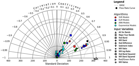
Figure 8.
Taylor Diagram of models developed for the Brazos River in this study.
As shown in Figure 8, there is a cluster of fifteen (15) models that perform significantly better than the remaining models based on their correlation coefficients. These models include the rating curve, the exponential relationship with the Red/Green Ratio input, the SVM with the Red Band input, and the twelve (12) machine learning algorithms with All Six Bands, Four Major Bands, Red/Green Ratio, and NIR Ratios as inputs. All these models perform in a relatively tight region of R and RSME values and can probably all be reasonably employed for the Brazos River. The three models that result in predictions with a standard deviation closest to the standard deviation of the test data set are the rating curve, the exponential relationship with the Red/Green Ratio as an input, and the SVM with the Red/Green Ratio as an input. In general, the four ELM and SVM models with All Six Bands, Four Major Bands, Red/Green Ratio, and NIR Ratios as inputs have the lowest average RSME compared to other algorithms.
3.2. Case Study
The exponential relationship with the Red/Green Ratio as an input, which was one of the best performing models developed during this study, was applied to the Brazos River and a portion of its estuary to estimate SSCs before, during, and after Hurricane Harvey. Hurricane Harvey was a catastrophic hurricane that lasted from 8/17/17 to 9/3/17 that made landfall on Texas near Houston on 8/30/17. This hurricane resulted in some of the highest, if not the highest, rainfall totals on record in the area and resulted in the highest daily mean flow rate over the data recorded for USGS-08116650 near Rosharon, TX, used in this study. Since Hurricane Harvey lasted so long, images for the months of August and September of 2017 were collected and processed.
Satellite images for both Landsat and Sentinel Mission 2 were collected and processed for this case study. The satellite images were clipped to the Brazos River and a portion of its estuary using aerial imagery. This assumed that the width of the river did not vary significantly during Hurricane Harvey and that the river has not changed course since 2017. Pixels labeled as medium- or high-confidence clouds, cloud shadows, ice, and snow based on the quality pixels provided by the satellite image’s source were removed. This resulted in a total of 28 images that could be used to estimate SSCs. Landsat Mission 9 was not included because it was not launched until 2021.
Some of the processed images did not result in many pixels with estimated SSCs following the filtering process. Thus, a general area just upstream (Area 1) and two miles downstream (Area 2) of the USGS-08116650 station were used to calculate the average SSCs estimated by the model to evaluate the model’s performance compared to field measurements over the case study area. The two general areas used to estimate the average SSCs near the USGS-08116650 gauge are shown in Figure 1. The estimated SSCs for pixels in these areas are shown in Figure 9. Only images where the majority of the pixels were not filtered out are shown in these figures. The images for the two areas show that the average estimated SSCs for these general areas are roughly the same for almost all the scenes. Only the scene on 9/6/17 shows a noticeable difference in average estimated SSCs between the two areas, where Area 1 has a value of 879 mg/L while Area 2 has a value of 742 mg/L.
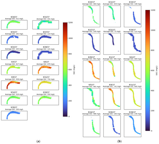
Figure 9.
Areas where model was applied to compare estimated SSCs with field data measurements before, during, and after Hurricane Harvey: (a) Estimated SSCs in Area 1, (b) Estimated SSCs in Area 2.
The model was also used to estimate SSCs in the Brazos River mouth and estuary. The model was only used for the estuary of the Brazos River on satellite images that were taken on the same days as the images used for Areas 1 and 2. An average estimated SSC was taken just downstream of the flood gates and just before the river discharges to the estuary for these images to compare to upstream averages in Areas 1 and 2. Figure 10 illustrates the estimated SSCs developed for the estuary of the Brazos River.
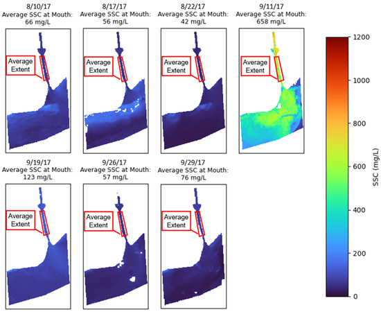
Figure 10.
Estimated SSC at the mouth and estuary of the Brazos River.
4. Discussion
Following the efforts made in this study, models that estimates SSCs through satellite imagery data for the Lower Brazos River near the Gulf of Mexico, Texas, U.S., using publicly available data were developed. The SSC estimators developed help improve our understanding of the sediment dynamics of the Brazos River and the river’s impact on the nearby San Bernard River. This understanding is discussed in more detail in the following paragraphs based on the case study, in which the exponential relationship with the Red/Green Ratio as an input was used to estimate SSCs before, during, and after Hurricane Harvey.
In general, the images of upstream Areas 1 and 2 show a decrease in estimated SSCs from 8/10/17 to 8/15/17, where SSCs are then consistent through 8/28/17. Following this period of consistent SSCs, the estimated SSCs were elevated from 8/30/17 to 9/19/17, with maximum values occurring on 8/30/17, 9/6/17, and 9/9/17. Following 9/19/17, the estimated SSCs were assumed to decrease, as the estimated SSCs on 9/26/17 returned to the levels seen from 8/15/17 to 8/28/17.
The images of upstream Areas 1 and 2 also show that the model can result in a wide range of estimated SSC values for a given satellite image in an area. This is more evident for higher SSC estimates. For example, the SSC estimates for Area 2 on 8/30/17 range from approximately 650 to 1000 mg/L. This could indicate that the model should not be used for inter-pixel relationships and should be used to estimate SSCs for a general area. Also, this inter-pixel variance is less prominent for lower SSCs, as shown by the estimates from 8/15/17 to 8/28/17 and estimates after 9/26/17.
The average estimated SSC developed for Areas 1 and 2 were compared to the daily mean flow and recorded SSCs at the USGS-08116650 station. Figure 11 shows this comparison. The recorded SSCs on 8/22/17 and 9/27/17 were collected at the TCEQ-16355 station, which is approximately the same location as the USGS-08116650 gauge. The estimated SSCs are nearly identical to field measurements taken before and after the large daily mean flow spike caused by Hurricane Harvey. Also, the estimated SSCs show a similar lag in response relative to the daily mean flow that is observed in the field data. However, the estimated SSC on 8/30/17 is about twice the field measurement. This vast difference could be a result of the difference in the timing of the satellite image and the collected field measurement, because during flood events, SSCs can vary dramatically. The estimated SSCs also show that the Brazos River continued to have elevated SSCs weeks after the flow spike caused by Hurricane Harvey. This delay in SSC reduction because of Hurricane Harvey is a similar response to that seen in the estimated SSC for the small flow spike on 8/9/17. During this smaller event, the estimated SSCs took up to a week to return to lower levels.
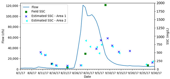
Figure 11.
Comparison of estimated SSCs to both daily mean flow and field SSC measurements.
In general, the estimated SSCs in the estuary and at the mouth of the Brazos River are lower than the SSCs estimated in upstream portions of the Brazos River. The reduction in average estimated SSCs from upstream to downstream could be a result of dilatation and sediment deposition between these locations. This is most evident for the images from 8/12/17 and 9/19/17, which experienced reductions in average estimated SSCs of 365 mg/L and 427 mg/L, respectively. Both days had relatively low daily mean flows, which is an indication of lower carrying capacity of the river. On 9/11/17, the average estimated SSC at the mouth of the Brazos River was only 58 mg/L lower than the average estimated SSC on the same day in the upstream locations. Also, on 9/11/17, the estimated SSC in the estuary indicates there was a plume of sediment leaving the Brazos River that was traveling west along the coast. On this day, the daily mean flow was significantly higher than the daily mean flows for all other images of the mouth and estuary developed. This higher flow can explain why for this day, the estimated SSCs show a plume of sediment at the mouth of the Brazos and a small reduction in estimated SSC from the upstream area to the mouth.
Again, images at the mouth and estuary of the Brazos River indicate that the model can lead to a wide variation in estimated SSCs between pixels. For example, in the images from 8/12/17 to 8/22/17, and the image on 9/29/17, the estimated SSCs show areas of low suspended sediment below 70 mg/L to areas of higher SSCs above 100 mg/L. This type of relationship is not expected unless sediment is introduced into the system and is likely a result of the interference of bottom reflectance from low water depth in the estuary caused by sand bars. In the image from 9/11/17, there are some dots of very low estimated SSCs, which are not realistic and could be a result of unfiltered cloud shadows as a result of mislabeled quality pixels. At a more zoomed-in scale, the estimated SSCs for some images produced with Sentinel Mission 2 show areas of lower SSCs in lines that resemble waves along the coast.
5. Conclusions
This study developed models that performed reasonably well at predicting SSCs in the Lower Brazos River. However, the models developed for this study had several limitations, as discussed in the following paragraphs.
The models developed for this study exhibited large inter-pixel variance when deployed to satellite image scenes along the Brazos River. Part of this variance was due to mislabeled quality pixels, boats navigating the river, and waves in the bay. However, in areas without these anomalies, the model showed high inter-pixel variance for areas where the estimated SSCs for pixel values that exceeded 1000 mg/L and areas of lower depth below the estimated SSCs for pixel values of 100 mg/L. In general, the models developed underpredicted SSCs above 1000 mg/L. Furthermore, for low SSCs and low-depth areas, the bottom reflectance could have saturated the surface reflectance measurements. This indicates that the models should be applied to evaluate SSCs in general areas and not evaluate relationships as fine as pixel-to-pixel. Furthermore, the model can be reasonably applied when the estimated SSCs range from 0 to 1000 mg/L, except for areas of low flow depth below SSCs of 100 mg/L.
In general, anomalies such as boats, clouds, and waves in the bay were observed to interfere with optical relationships being developed to estimate SSCs. This study tried to handle clouds by using quality pixels from space agencies, but this was not a perfect filtering method. Other anomalies were not directly handled in this study. Furthermore, cloud cover limits the application of models developed for this study in areas that experience many days of cloud cover or during prolonged storm events. These models would also not be applicable in areas with prolonged ice cover on the river.
The models developed for this study used satellite image data with pixel resolutions ranging from 10 m to 30 m. This limits our ability to apply the models in further upstream portions of the river. Assuming a pixel encompasses only the river, the models could be deployed for rivers as narrow as 10 m (33 ft) if images with a 10 m pixel resolution are available or as narrow as 30 m (100 ft) if images with a 30 m pixel resolution are available. This best-case scenario would require the pixel and river reach to line up exactly to be a pure water pixel. This is rarely the case, and it is generally accepted that satellite images should be used on rivers that are at least three times the width of the pixel resolution to guarantee at least one pure water pixel. These models result in rivers as narrow as 30 m (100 ft) if images with a 10 m pixel resolution are available or as narrow as 90 m (300 ft) if images with a 30 m pixel resolution are available.
Future studies can investigate the following to further the findings documented in this study:
- Utilizing satellite images and corresponding SSC pairs collected on the same date, preferably at the same time. This could include the redevelopment of the models in this study with this restriction to examine whether performance improves.
- Applying the models developed in this study to rivers similar to the Brazos River which experience comparable flows, SSC ranges, and sediment types, to evaluate their applicability beyond the Brazos River.
- Using higher-resolution satellite image data to allow for the use of the developed models further upstream in the Brazos River. This would also involve evaluating whether this higher resolution is comparable to the data used in this study, thus facilitating the use of a larger dataset for model development.
- Developing a more physically/mathematically derived relationship between satellite image reflectance values and SSCs. Such relationships have been previously developed for depth estimation in waterbodies.
Author Contributions
This paper was conceptualized by T.S. and H.A.; the methodology was formulated by T.S. and H.A; Landsat Missions 4–9 and Sentinel Mission 2 satellite imagery and USGS and TCEQ data were processed by T.S. This study used Python open-source languages for modeling and image processing. All authors have read and agreed to the published version of the manuscript.
Funding
This research received no external funding.
Data Availability Statement
The original contributions presented in the study are included in the article, further inquiries can be directed to the corresponding author.
Conflicts of Interest
The authors declare no conflicts of interest.
References
- Sobel, R.S.; Kiaghadi, A.; Rifai, H.S. Modeling water quality impacts from hurricanes and extreme weather events in urban coastal systems using Sentinel-2 spectral data. Environ. Monit. Assess. 2020, 192, 307. [Google Scholar] [CrossRef] [PubMed]
- Coonrod, J.E.A. Suspended Sediment Yield in Texas Watersheds; The University of Texas at Austin: Austin, TX, USA, 1998. [Google Scholar]
- Walling, D.E.; Moorehead, P.W. The particle size characteristics of fluvial suspended sediment: An overview. In Sediment/Water Interactions: Proceedings of the Fourth International Symposium; Springer: Dordrecht, The Netherlands, 1989; pp. 125–149. [Google Scholar]
- Poesen, J.W.; Vandaele, K.; Van Wesemael, B. Contribution of gully erosion to sediment production on cultivated lands and rangelands. IAHS Publ.-Ser. Proc. Rep.-Intern. Assoc. Hydrol. Sci. 1996, 236, 251–266. [Google Scholar]
- Lefrançois, J.; Grimaldi, C.; Gascuel-Odoux, C.; Gilliet, N. Suspended sediment and discharge relationships to identify bank degradation as a main sediment source on small agricultural catchments. Hydrol. Process. Int. J. 2007, 21, 2923–2933. [Google Scholar] [CrossRef]
- Droppo, I.G.; Nackaerts, K.; Walling, D.E.; Williams, N. Can flocs and water stable soil aggregates be differentiated within fluvial systems? Catena 2005, 60, 1–18. [Google Scholar] [CrossRef]
- Peterson, K.T.; Sagan, V.; Sidike, P.; Cox, A.L.; Martinez, M. Suspended sediment concentration estimation from landsat imagery along the lower missouri and middle Mississippi Rivers using an extreme learning machine. Remote Sens. 2018, 10, 1503. [Google Scholar] [CrossRef]
- Reisinger, A.; Gibeaut, J.C.; Tissot, P.E. Estuarine suspended sediment dynamics: Observations derived from over a decade of satellite data. Front. Mar. Sci. 2017, 4, 233. [Google Scholar] [CrossRef]
- Foster, I.D.L.; Millington, R.; Grew, R.G. The impact of particle size controls on stream turbidity measurement; some implications for suspended sediment yield estimation. Eros. Sediment Transp. Monit. Programmes River Basins 1992, 210, 51–62. [Google Scholar]
- Jastram, J.D.; Zipper, C.E.; Zelazny, L.W.; Hyer, K.E. Increasing precision of turbidity-based suspended sediment concentration and load estimates. J. Environ. Qual. 2010, 39, 1306–1316. [Google Scholar] [CrossRef] [PubMed]
- Minella, J.P.G.; Merten, G.H.; Reichert, J.M.; Clarke, R.T. Estimating suspended sediment concentrations from turbidity measurements and the calibration problem. Hydrol. Process. Int. J. 2008, 22, 1819–1830. [Google Scholar] [CrossRef]
- Sari, V.; Castro, N.M.d.R.; Pedrollo, O.C. Estimate of suspended sediment concentration from monitored data of turbidity and water level using artificial neural networks. Water Resour. Manag. 2017, 31, 4909–4923. [Google Scholar] [CrossRef]
- Afan, H.A.; El-Shafie, A.; Mohtar, W.H.M.W.; Yaseen, Z.M. Past, present and prospect of an Artificial Intelligence (AI) based model for sediment transport prediction. J. Hydrol. 2016, 541, 902–913. [Google Scholar] [CrossRef]
- Rajaee, T.; Jafari, H. Two decades on the artificial intelligence models advancement for modeling river sediment concentration: State-of-the-art. J. Hydrol. 2020, 588, 125011. [Google Scholar] [CrossRef]
- Legleiter, C.J.; Kinzel, P.J.; Overstreet, B.T. Evaluating the potential for remote bathymetric mapping of a turbid, sand-bed river: 1. Field spectroscopy and radiative transfer modeling. Water Resour. Res. 2011, 47, W09531. [Google Scholar] [CrossRef]
- Mishra, D.R.; Narumalani, S.; Rundquist, D.; Lawson, M. Characterizing the vertical diffuse attenuation coefficient for downwelling irradiance in coastal waters: Implications for water penetration by high resolution satellite data. ISPRS J. Photogramm. Remote Sens. 2005, 60, 48–64. [Google Scholar] [CrossRef]
- Lyzenga, D.; Malinas, N.; Tanis, F. Multispectral bathymetry using a simple physically based algorithm. IEEE Trans. Geosci. Remote Sens. 2006, 44, 2251–2259. [Google Scholar] [CrossRef]
- Phillips, J.D. Geomorphic Context, Constraints, and Change in the Lower Brazos and Navasota Rivers, Texas; Copperhead Road Geoscience: Lexington, KY, USA, 2006. [Google Scholar]
- Strom, K.; Hosseiny, H. Suspended Sediment Sampling and Annual Sediment Yield on the Middle Trinity River; University of Houston, Department of Civil and Environmental Engineering: Houston, TX, USA, 2015. [Google Scholar]
- Texas Commission on Environmental Quality. Monitoring Operations Division. Surface Water Quality Monitoring Procedures, Volume 1: Physical and Chemical Monitoring Methods; Texas Commission on Environmental Quality: Austin, TX, USA, 2008.
- U.S. Geological Survey. USGS EROS Archive—Sentinel-2—Comparison of Sentinel-2 and Landsat. Available online: https://www.usgs.gov/centers/eros/science/usgs-eros-archive-sentinel-2-comparison-sentinel-2-and-landsat (accessed on 28 June 2023).
- Burkov, A. The Hundred-Page Machine Learning Book; Andriy Burkov: Orlando, FL, USA, 2023. [Google Scholar]
- Burkov, A. Machine Learning Engineering; True Positive Incorporated: Montreal, QC, Canada, 2020; Volume 1. [Google Scholar]
- Huang, G.-B.; Zhu, Q.-Y.; Siew, C.-K. Extreme learning machine: Theory and applications. Neurocomputing 2006, 70, 489–501. [Google Scholar] [CrossRef]
- Taylor, K.E. Summarizing multiple aspects of model performance in a single diagram. J. Geophys. Res. Atmos. 2001, 106, 7183–7192. [Google Scholar] [CrossRef]
- Chen, S.; Han, L.; Chen, X.; Li, D.; Sun, L.; Li, Y. Estimating wide range Total Suspended Solids concentrations from MODIS 250-m imageries: An improved method. ISPRS J. Photogramm. Remote Sens. 2015, 99, 58–69. [Google Scholar] [CrossRef]
- Pereira, L.S.F.; Andes, L.C.; Cox, A.L.; Ghulam, A. Measuring suspended-sediment concentration and turbidity in the middle Mississippi and lower Missouri rivers using landsat data. JAWRA J. Am. Water Resour. Assoc. 2018, 54, 440–450. [Google Scholar] [CrossRef]
Disclaimer/Publisher’s Note: The statements, opinions and data contained in all publications are solely those of the individual author(s) and contributor(s) and not of MDPI and/or the editor(s). MDPI and/or the editor(s) disclaim responsibility for any injury to people or property resulting from any ideas, methods, instructions or products referred to in the content. |
© 2024 by the authors. Licensee MDPI, Basel, Switzerland. This article is an open access article distributed under the terms and conditions of the Creative Commons Attribution (CC BY) license (https://creativecommons.org/licenses/by/4.0/).