Article

HGR Correlation Pooling Fusion Framework for Recognition and Classification in Multimodal Remote Sensing Data

Tsinghua Shenzhen International Graduate School, Tsinghua University, Shenzhen 518055, China
*
Author to whom correspondence should be addressed.
Remote Sens. 2024, 16(10), 1708; https://doi.org/10.3390/rs16101708
Submission received: 20 March 2024 / Revised: 8 May 2024 / Accepted: 9 May 2024 / Published: 11 May 2024

Abstract

:
This paper investigates remote sensing data recognition and classification with multimodal data fusion. Aiming at the problems of low recognition and classification accuracy and the difficulty in integrating multimodal features in existing methods, a multimodal remote sensing data recognition and classification model based on a heatmap and Hirschfeld–Gebelein–Rényi (HGR) correlation pooling fusion operation is proposed. A novel HGR correlation pooling fusion algorithm is developed by combining a feature fusion method and an HGR maximum correlation algorithm. This method enables the restoration of the original signal without changing the value of transmitted information by performing reverse operations on the sample data. This enhances feature learning for images and improves performance in specific tasks of interpretation by efficiently using multi-modal information with varying degrees of relevance. Ship recognition experiments conducted on the QXS-SROPT dataset demonstrate that the proposed method surpasses existing remote sensing data recognition methods. Furthermore, land cover classification experiments conducted on the Houston 2013 and MUUFL datasets confirm the generalizability of the proposed method. The experimental results fully validate the effectiveness and significant superiority of the proposed method in the recognition and classification of multimodal remote sensing data.

1. Introduction

In practical applications, there are certain limitations in the information content, resolution, and spectrum of single-mode scenes, making it difficult to meet the application requirements [1,2,3]. Multimodal image fusion has become an attractive research direction. Recently, with the in-depth research of fusion algorithms, multimodal recognition technology has made rapid progress [4,5,6]. The multimodal multi-tasking basic model has been widely studied in the field of computer vision. It combines image data with text or speech data as multimodal input and sets different pre-training tasks for different modal branches to enable the model to learn and understand the information between modalities. Multimodal fusion can improve the recognition rate and has better robustness and stability [7], further promoting the development of multimodal image fusion technology. At present, image fusion has been widely used in remote sensing image fusion [8], visible and infrared image fusion [9] multi-focus image fusion [10], multi-exposure image fusion [11], medical imaging fusion [12], etc.
In recent years, marine ship detection has been extensively used in many fields such as fishery management and navigation supervision. Determining how to achieve accurate detection through multimodal fusion of marine ships has great strategic significance in both civil and military fields. Thus, Cao et al. [13] proposed a ship recognition method based on morphological watershed image segmentation and Zemyk moments for ship extraction and recognition in video surveillance frame images. Wang et al. [14] developed a SAR ship recognition method based on multi-scale feature attention and an adaptive weighted classifier. Zhang et al. [15] presented a fine-grained ship image recognition network based on the bilinear convolutional neural network (BCNN). Han et al. [16] proposed a new efficient information reuse network (EIRNet), and based on EIRNet, they designed a dense feature fusion network (DFF-Net), which reduces information redundancy and further improves the recognition accuracy of remote sensing ships. Liu, Chen, and Wang [17] fused optical images with SAR images, utilized feature point matching, contour extraction, and brightness saliency to detect ship components, and identified ship target types based on component information voting results. It is challenging to realize information separation under maximum use of information without compromising image quality.
Meanwhile, in the past decade, the application of remote sensing based on deep learning has made significant advancements in object detection, scene classification, land use segmentation, and recognition. This is mainly because deep neural networks can effectively map remote sensing observations into the needed geographic knowledge through their strong feature extraction and representation capabilities [18,19,20]. Existing remote sensing interpretation methods mainly adopt manual visual interpretation and semi-automatic techniques based on accumulated expert knowledge, showing high accuracy and reliability. Artificial intelligence technology represented by deep learning is widely used in remote sensing image interpretation [21] and has greatly improved the efficiency of remote sensing data interpretation. For instance, entropy decomposition was utilized to identify crops from synthetic aperture radar (SAR) images [22]. Similarly, normative forests were used to classify hyperspectral images [23]. Jafarzadeh et al. [24] employed several tree-based classifiers’ bagging and boosting sets to classify SAR, hyperspectral, and multispectral images.
Compared to single sensors, multi-sensor or remote sensing data provides different descriptions of ground objects, thereby providing richer information for various application tasks. In the field of remote sensing, modality can usually be regarded as the imaging results of the same scene and target under different sensors, and using multimodal data for prediction and estimation is a research hotspot in this field. Given this, an integration method using intensity tone saturation (IHS) transform and wavelet was adopted to fuse SAR images with medium-resolution multispectral images (MSIs) [25]. Cao et al. [26] proposed a method for monitoring mangrove species using rotating forest fusion HSI and LiDAR images. Hu et al. [27] developed a fusion method for PolSAR and HSI data, which extracts features from the two patterns at the target level and then fuses them for land cover classification. Li et al. [28] introduced an asymmetric feature fusion idea for hyperspectral and SAR images. This idea can be extended to the fields of hyperspectral and LiDAR images. Although the above studies have realized the fusion of multiple remote sensing data, designing the loss function specifically needs further investigation. Multimodal data fusion [29,30] is one of the most promising research directions for deep learning in remote sensing, particularly when SAR and optical data are combined because they have highly different geometrical and radiometric properties [31,32].
Meanwhile, the Hirschfeld–Gebelein–Rényi (HGR) maximum correlation [33] has been widely used as an information metric for studying inference and learning problems [34]. In the field of multimodal fusion based on HGR correlation, Liang et al. [35] introduced the HGR maximum correlation terms into the loss function for person recognition in multimodal data. Wang et al. [36] proposed Soft-HGR, a novel framework to extract informative features from multiple data modalities. Ma et al. [37] developed an efficient data augmentation framework by designing a multimodal conditional generative adversarial network (GAN) for audiovisual emotion recognition. However, the values of the transmitted data are changed in the data fusion process.
Inspired by previous studies, the issues of remote sensing data recognition and classification with multimodal data fusion are studied. The main innovations of this article are stated as follows:
(1)
An HGR correlation pooling fusion algorithm is developed by integrating a feature fusion method with an HGR correlation algorithm. This framework adheres to the principle of relevance correlation and segregates information based on its intrinsic relevance into distinct classification channels. It enables the derivation of loss functions for positive, zero, and negative samples. Then, a tailored overall loss function is designed for the model, which significantly enhances feature learning in multimodal images.
(2)
A multimodal remote sensing data recognition and classification model is proposed, which can achieve information separation under maximum utilization. The model enhances the precision and accuracy of target recognition and classification while preserving image information integrity and image quality.
(3)
The HGR pooling specifically addresses multimodal pairs (vectors) and intervenes in the information transmission process without changing the value of the transmitted information. It enables inversion operations on positive, zero, and negative sample data in the original signal of the framework, thereby supporting traceability for the restoration of the original signal. This advancement greatly improves the interpretability of the data.

2. Related Work

To date, multimodal data fusion has been widely used in remote sensing [2,38]. In most cases, multimodal data recognition systems are much more accurate than the corresponding optimal single-modal data recognition systems [39]. According to the fusion level, the fusion strategies between various modalities can be mainly divided into data-level fusion, feature-level fusion, and decision-level fusion [40]. Data-level fusion is aimed at the data without special processing for each mode. The original data of each mode is combined without pretreatment to obtain the data after the mode function. Finally, the fusion data are taken as the input of the identification network for training or identification. Feature-level fusion concatenates the features of each modality into a large feature vector, which is then fed into a classifier for classification and recognition. Decision-level fusion determines the weights and fusion strategies of each modality based on their credibility after obtaining the prediction probability through a classifier, and then it obtains the fused classification results.
The complexity of the above three fusion strategies decreases in sequence, and their dependence on the rest of the system processes increases in sequence. Usually, multimodal fusion strategies are selected based on specific situations. With the improvement in hardware computing power and the increasing demand for applications, the studies of data recognition, which contains massive data information and has mature data collection methods, are constantly enriched.
In order to ascertain the degree of correlation and to identify the most informative features, the Hirschfeld–Gebelein–Rényi (HGR) maximal correlation is employed as a normalized measure of the dependence between two random variables. This has been widely applied as an information metric to study inference and learning problems. In [33], the sample complexity of estimating the HGR maximal correlation functions comes from the alternating conditional expectation algorithm using training samples from large datasets. By using the HGR maximal correlation in [37], the high dependence between the different modalities in the generated multimodal data is modeled. In this way, it exploits different modalities in the generated data to approximate the real data. Although these studies have yielded promising outcomes, it is difficult to achieve accurate detection through multimodal fusion of marine ships, and the interrelationships between modules have not been fully elucidated.
Feature-level fusion can preserve more data information. It first extracts features from the image and then performs fusion. Pedergnana et al. [41] used optical and LiDAR data by extracting extended attribute contours of the two modalities and connecting them with the original modalities. Then, a two-layer DBN network structure was proposed, which first learns the features of the two modalities separately and then connects the features of the two modalities to learn the second layer. Finally, a support vector machine (SVM) is utilized to evaluate and classify the connected features [42].
However, feature-level fusion requires high computing power and is prone to the curse of dimensionality, and the application of decision-level fusion is also common. To address these issues, a SAR and infrared fusion scheme based on decision-level fusion was introduced [43]. This scheme uses a dual-weighting strategy to measure the confidence of offline sensors and the reliability of online sensors. The structural complexity of decision-level fusion is relatively low and does not require strict temporal synchronization, which performs well in some application scenarios.

3. Methodology

In this section, the details of the proposed CNN-based special HGR correlation pooling fusion framework for multimodal data are introduced. The framework can preserve adequate multimodal information and extract the correlation between modal 1 and modal 2 data so that discriminative information can be learned more directly.

3.1. Problem Definition

Given paired observations from multimodal data {(x(i), y(i))|x(i)Rn1, y(i)Rn2, i = 1, …, N}, let x and y represent the modal 1 image and modal 2 image with dimensionalities Rn1 and Rn2, respectively. The ith components x(i)x, y(i)y match each other and come from the same region, while the ith component x(i)x and the jth component y(j)y do not match each other and come from different regions.

3.2. Model Overview

In this paper, to solve the problems of low recognition and classification accuracy and difficulty in effectively integrating multimodal features, an HGR maximal correlation pooling fusion framework is proposed for recognition and classification in multimodal remote sensing data. The overall structure of the framework is shown in Figure 1. In the subsequent subsections, the model will be discussed in detail.
For multimodal image pairs, the framework has two separate feature extraction networks. To reduce the dimensionality of features, following the feature extraction backbone, a 1 × 1 convolution layer is used, and the modal 1 feature map and modal 2 feature map are obtained separately. Then, a special HGR maximal correlation pooling layer is employed. The HGR pooling handles multimodal pairs (vectors) and only intervenes in the information transmission without changing the value of the transmitted information. The principle is to filter the values of information with different relevant characteristics and transmit them to the corresponding subsequent classification channels. The feature data are processed to obtain positive sample data, zero sample data, and negative sample data for modal 1 and modal 2 features, respectively. Then, the three types of sample data from modal 1 and modal 2 are input into the ResNet50 [44] network to extract feature vectors, and feature level fusion is performed on the corresponding feature vectors to obtain fused positive samples, fused zero samples, and fused negative samples.
Finally, the positive, zero, and negative samples of modal 1/modal 2 images are fused respectively using the recognition and classification network, thereby accomplishing multimodal recognition tasks.

3.3. Heatmap and HGR Correlation Pooling

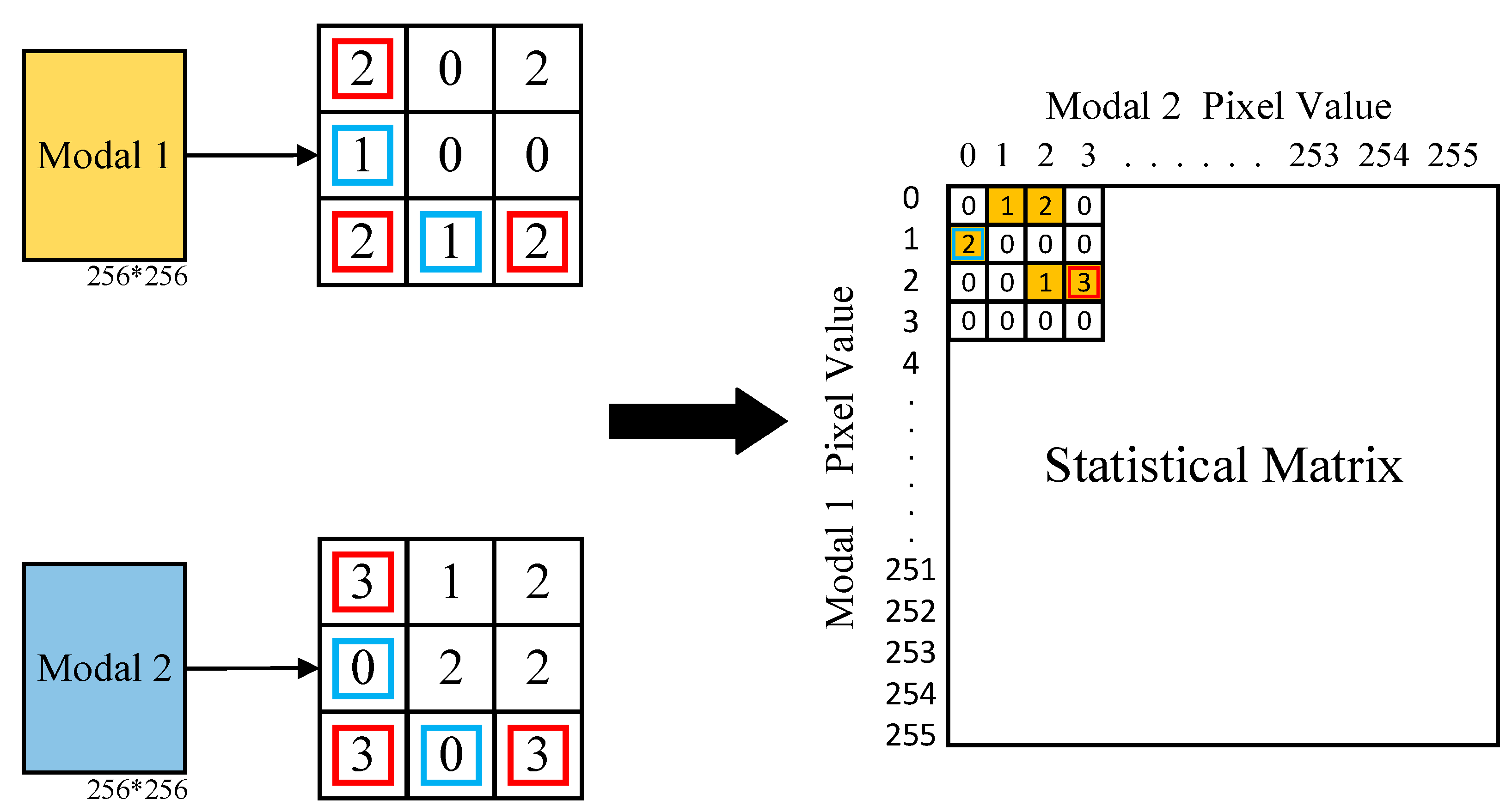
The input set of multimodal images needs to be pre-aligned to generate heatmaps. X denotes the input data of modal 1 pixel matrix of size n × n , and Y denotes the input data of modal 2 pixel matrix of size n × n . The statistical matrices of modal 1 and modal 2 images are illustrated by empirical distributions and defined as follows:
For each pixel of modal 1 and modal 2 images:
X ( p s , x ) = ( # o f p s i n x ) = i = 1 n 1 { x i = p s }
Y ( p o , y ) = ( # o f p o i n y ) = i = 1 n 1 { y i = p o }
where ps and po represent the pixel position in each modal 1 and modal 2 image, respectively, and # represents the number of pixels in modal 1 and modal 2 images. The expressions appear to be defining functions X(ps,x) and Y(po,y), which count the occurrences of specific pixel positions ps and po in two different modal images, respectively.
According to the definition of X and Y, the statistical matrix calculation process is as follows:
D s = F s ( X , Y )
where F s ( ) is the statistical matrix calculation function and Ds is the statistical matrix. The calculation of the statistical matrix process is shown in Figure 2.
Then, the pixel-level maximal nonlinear cross-correlation between sets is given by:
ρ ( x , y ) = max E [ f ( x ) ] = 0 , E [ g ( y ) ] = 0 V a r { f ( x ) ] = 1 , V a r [ g ( y ) ] = 1 E [ f ( x ) g ( y ) ]
H = f ( x ) g ( y )
where f(x) represents modal 1 in each pixel position, g(y) represents modal 2 in each pixel position, and H represent the nonlinear correlation between the pixel points in modal 1 and modal 2 images.
According to the obtained statistical matrix, the HGR cross-correlation is calculated as follows:
F H G R ( D s ) = [ f ( x ) , g ( y ) ] T
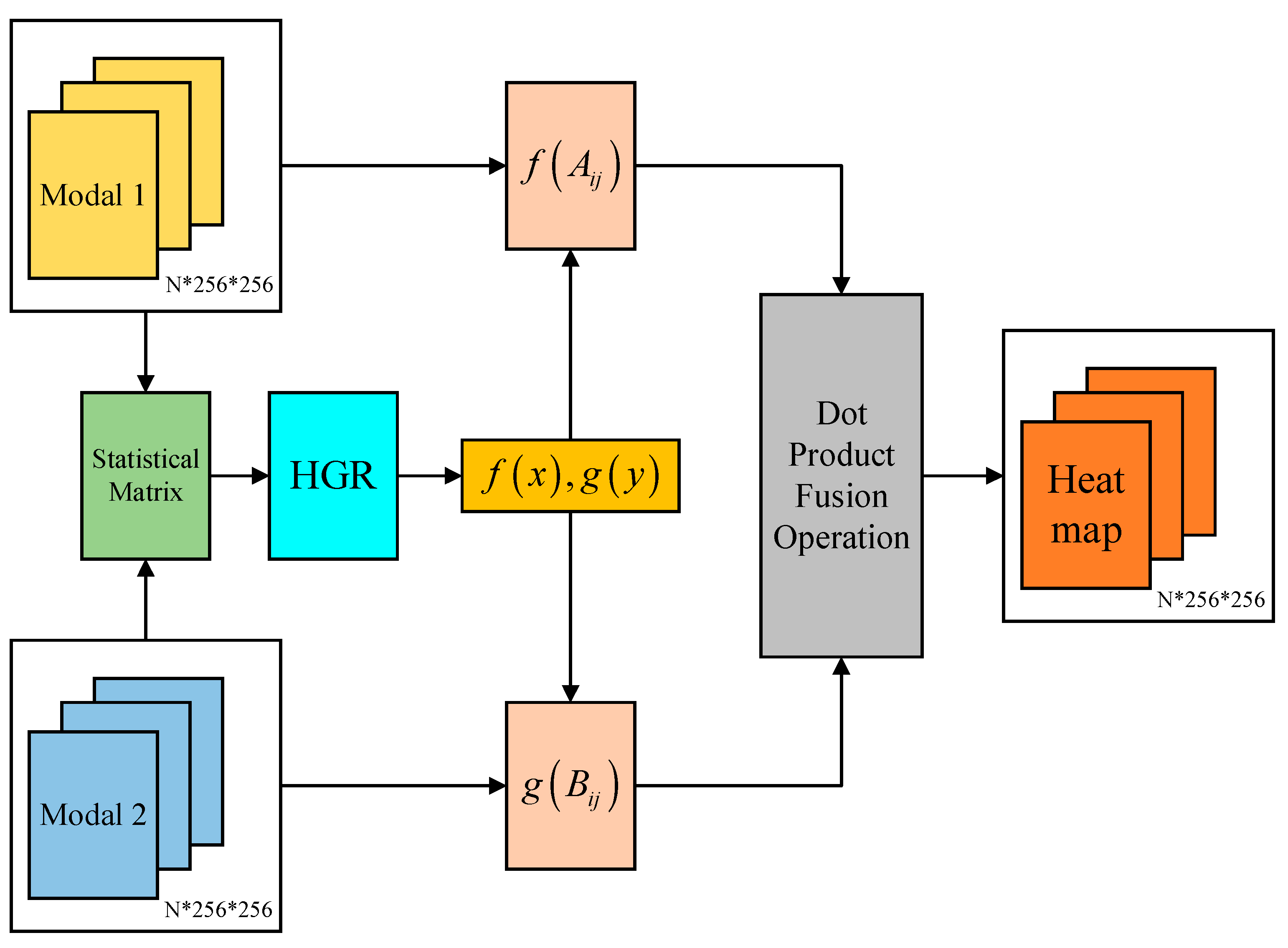
where F H G R ( ) is the HGR cross-correlation calculation function, and f(x) and g(y) are projection vectors. Based on the obtained projection vector, the heatmap pixel matrix is calculated as follows:
D H M = f ( X i j ) g ( Y i j ) , i , j { 1 , 2 , , n }
where D H M is a heatmap pixel matrix of size n × n . The heatmap calculation process is shown in Figure 3.
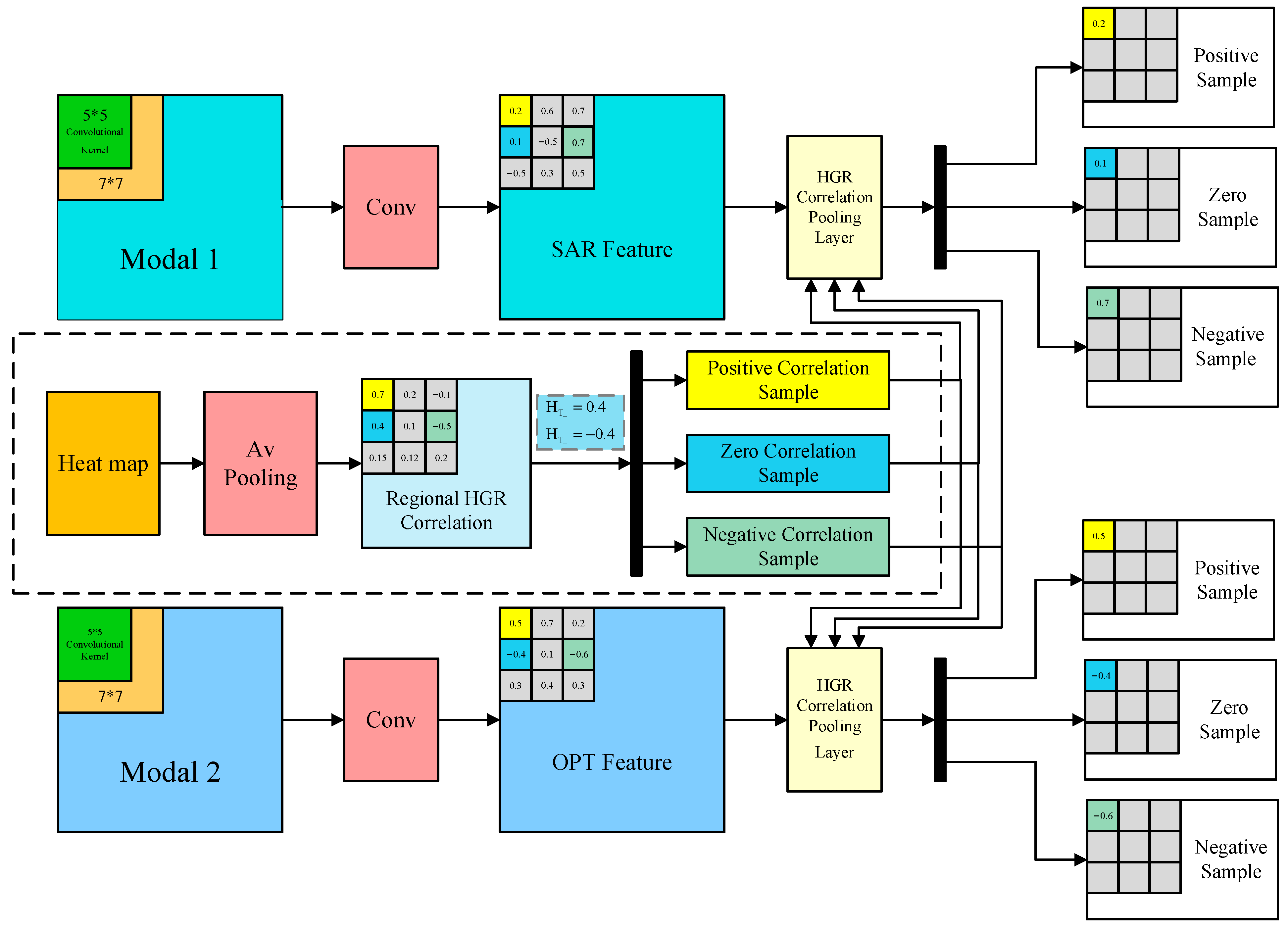
Based on the heatmap pixel matrix obtained above, the average pooling is calculated as follows:
B = A P ( D H M )
where A P ( ) is the average pooling function, and B is the HGR region cross-correlation matrix of size ( n 2 ) × ( n 2 ) . Furthermore, the calculation of cross-correlation positive, zero, and negative sample matrices can be expressed as:
B + = B k l , B k l 0.4 0 , B k l < 0.4
B 0 = B k l , B k l < 0.4 0 , B k l 0.4
B = B k l , B k l 0.4 0 , B k l > 0.4
where k , l { 1 , 2 , , n 2 } , and B + , B 0 , and B represent positive, zero, and negative cross-correlation sample matrices, respectively. The calculation of the HGR cross-correlation sample matrix is shown in Figure 4.
Meanwhile, A is defined as the image pixel position matrix, and max is defined as the matrix maximum pooling dot product operation. Based on the cross-correlation positive, zero, and negative sample matrix obtained by the above calculation, the maximum pooling calculation process is given by:
R + = A max B + R 0 = A max B 0 R = A max B
where R + , R 0 , and R are HGR cross-correlation positive, zero, and negative sample matrix maximum pooling results, respectively. The HGR cross-correlation pooling process is shown in Figure 5.
Finally, for the special HGR maximum correlation pooling layer, the key point is to obtain the transfer position based on the generated correlation matrix and transfer the values corresponding to the intermediate matrix in the pooling process. Due to dimensionality reduction, instead of relying on the common maximum value, only one value is passed on for 3 × 3, and correlation is used for transfer.
As shown in Figure 6, the corresponding modal 1/modal 2 features are transmitted through the special HGR pooling layer, which intervenes in the information transmission based on the HGR maximum correlation matrix instead of normal pooling methods without changing the value of the transmitted information. Meanwhile, the modal 1/modal 2 feature maps are divided into positive samples, zero samples, and negative samples for modal 1 and modal 2 data, respectively.

3.4. Learning Objective

The cross-entropy loss and the Soft-HGR loss with modified weights are taken as the loss for the whole network. Thus, the learning objective of the framework can be represented as:
L = L c e + α L S o f t H G R
where Lce represents the cross-entropy loss and Lsoft-HGR denotes the Soft-HGR loss. α is the penalty parameter to balance the cross-entropy loss Lce and the Soft-HGR loss Lsoft-HGR, which are designer-defined parameters ranging from 0 to 1.
The cross-entropy loss Lce is used to measure the difference between the predicted result y ^ i and the ground-truth label y i , and can be expressed as follows:
L c e = 1 n i = 1 n [ y i log y ^ i + ( 1 y i ) log ( 1 y ^ i ) ]
The Soft-HGR loss Lsoft-HGR [36] is utilized to maximize the correlation between multimodal images, and can be represented as follows:
L S o f t H G R = α 1 L p o s i t i v e + α 2 L z e r o + ( 1 α 1 α 2 ) L n e g a t i v e
where α 1 and α 2 are weighting factors, which are designer-defined parameters ranging from 0 to 1. Lpositive, Lzero, and Lnegative represent the loss for positive samples, zero samples, and negative samples, and their definitions are given below:
L p o s i t i v e = s . t . , E f P = 0 , c o v ( f P ) = I     E g P = 0 , c o v ( g P ) = I E f P T X g P Y 1 2 t r ( c o v ( f P ( X ) ) c o v ( g P ( Y ) ) )
L z e r o = s . t . , E f Z = 0 , c o v ( f Z ) = I     E g Z = 0 , c o v ( g Z ) = I E f Z T X g Z Y 1 2 t r ( c o v ( f Z ( X ) ) c o v ( g Z ( Y ) ) )
L n e g a t i v e = s . t . , E f N = 0 , c o v ( f N ) = I     E g N = 0 , c o v ( g N ) = I E f N T X g N Y 1 2 t r ( c o v ( f N ( X ) ) c o v ( g N ( Y ) ) )
where fp(X) and gp(Y) represent a pair of positive samples. Similarly, fZ(X) and gZ(Y) represent a pair of zero samples, and fN(X) and gN(Y) represent a pair of negative samples. As a supplement, the expectations and covariance are approximated through the sample mean and sample covariance.

4. Experiments and Analysis

4.1. Dataset

The ship recognition experiments were conducted on the QXS-SROPT dataset, and the land cover classification experiments were conducted on the Houston 2013 and MUUFL datasets to verify the effectiveness of the proposed model and test the improvement in remote sensing data recognition and classification when maximizing the utilization of multimodal information.
QXS-SAROPT [45] contains 20,000 pairs of optical and SAR images collected from Google Earth remote sensing optical images and GaoFen-3 high-resolution spotlight images. The size of each image is 256 × 256 to fit the neural network with a resolution of 1 m. This dataset covers San Diego, Shanghai, and Qingdao.
The HSI-LiDAR Houston2013 dataset [46], provided for IEEE GRSS DFC2013, consists of imagery collected by the ITRES CASI-1500 imaging sensor. This imagery encompasses the University of Houston campus and its adjacent rural areas in Texas, USA. This dataset is widely used for land cover classification.
The HSI-LiDAR MUUFL dataset was constructed over the campus of the University of Southern Mississippi using the Reflective Optics System Imaging Spectrometer (ROSIS) sensor [47,48]. This dataset contains HSI and LiDAR data and is widely used for land cover classification.

4.2. Data Preprocessing and Experimental Setup

Since the image pairs in the QXS-SROPT dataset do not contain labels and are not aligned, in this study, manual alignment operations were performed on 131 image pairs. The proposed model learns the corresponding pixel correlation from SAR and optical image pairs, and calculates the maximum pixel-level HGR cross-correlation between SAR-optical datasets and the corresponding projection vectors f (x), g (y) to generate the heatmap and HGR cross-correlation pooling matrix modules. The pixel-level HGR has a certain potential for improving network multimodal information learning.
In the Houston 2013 dataset [46], the HSI image contains 349 × 1905 pixels and features 144 spectral channels at a spectral resolution of 10 nm, spanning a range from 364 to 1046 nm. Meanwhile, LiDAR data for a single band provide elevation information for the same image area. The study scene encompasses 15 distinct land cover and land use categories. This dataset contains 2832 training samples and 12,197 test samples, as listed in Table 1 [49].
In the MUUFL dataset [48], the HSI image contains 325 × 220 pixels, covering 72 spectral bands. The LiDAR imagery incorporates elevation data across two grids. Due to noise considerations, 8 initial and final bands were discarded, and 64 bands remained. The data encompass 11 urban land cover classes, comprising 53,687 ground truth pixels. Table 2 presents the distribution of 5% samples randomly extracted from each category.
The proposed model was trained using the Lion optimizer for 500 epochs and a batch size of 32 with an initial learning rate of 0.0001. After 30 epochs, the learning rate gradually decreased by 1 × 10−0.01 times in each epoch. All experiments were conducted on a computer equipped with an Intel(R) Xeon(R) Gold 6133 CPU @ 2.50 GHz and an NVIDIA GeForce RTX3090 GPU (NVIDIA, Santa Clara, CA, USA) with 24 G memory, 64-bit Ubuntu 20.04 operating system, CUDA 12.2, and cuDNN 8.8. The source code was implemented using PyTorch 2.1.1 and Python 3.9.16.

4.3. Ship Recognition Experiment

To verify the performance of the proposed HGRPool method, a series of experiments were conducted on the QXS-SAROPT dataset (100 training samples with 4358 instances, 31 testing samples with 1385 instances) to perform ship feature recognition on SAR–optical image pairs. The results of three experiments are illustrated in Figure 7, Figure 8 and Figure 9, where (a) illustrates the optical image, (b) shows the heatmap, (c) displays the SAR image, and (d) depicts the ship recognition results. The results from these figures demonstrate that the HGRPool method effectively identifies different ships, achieving commendable recognition performance and effectively distinguishing water bodies.
The proposed HGRPool method was compared with the BNN method proposed by Bao et al. [50]. Table 3 lists the values of four commonly used indicators, namely precision (P), recall (R), F1-score (F1), and accuracy (Acc) for the recognition results. Meanwhile, under the same experimental conditions, comparative experiments were conducted with other existing methods, including MoCo-BNN [51], CCR-Net [2], and MFT [52]. The experimental data are presented in Table 3. The precision, recall, F1-score, and accuracy of the proposed method reached 0.908, 0.988, 0.946, and 0.898, respectively. The proposed method achieved better results than existing methods, especially in terms of accuracy. The results suggest that the proposed method has greater recognition stability and accuracy and higher localization accuracy.

4.4. Information Traceability Experiment

To demonstrate information integrity throughout the processing stages, an information traceability experiment was conducted using images in three distinct forms: positive, negative, and zero. The experiment aimed to retrieve the original images based on these three forms. This part of the experiment involved six sets of tests, three with optical images and three with SAR images. The results are illustrated in Figure 10, Figure 11, Figure 12, Figure 13, Figure 14 and Figure 15. In these figures, (a) represents the positive image, (b) the negative image, (c) the zero image, and (d) the target traceability result image. From Figure 10, Figure 11, Figure 12, Figure 13, Figure 14 and Figure 15, it can be observed that the traced images are consistent with the original images, with no information loss. This indicates that the proposed algorithm maintains information integrity throughout the processing stages, ensuring that no information is lost.

4.5. Land Cover Classification Experiment on the Houston 2013 Dataset

To validate the generalizability of the method proposed in this paper, land cover classification experiments were conducted on the Houston 2013 dataset. Our method was compared with traditional machine learning algorithms and state-of-the-art methods in the field of deep learning, including CCF [53], CoSpace [54], Co-CNN [55], FusAT-Net [56], ViT [57], S2FL [49], Spectral-Former [58], CCR-Net [2], MFT [52], and DIMNet [59]. The specific results are shown in Figure 16, where (a) displays the DSM of LiDAR data, (b) shows the heatmap, (c) represents the three-band color composite for HSI spectral information, (d) shows the train ground-truth map, (e) shows the test ground-truth map, and (f) illustrates the classification results, with good contrast post-reconstruction. The values of three universal indicators, namely overall accuracy (OA), class accuracy (AA), and Kappa coefficient, are presented in Table 4 for comparison, where the top outcomes are highlighted in bold. It is evident that our method outperforms the others in terms of OA (92.23%), AA (93.55%), and Kappa coefficient (0.9157). It surpasses other methods in eight categories (stressed grass, synthetic grass, water, residential, road, parking lot 1, tennis court, and running track), especially achieving the highest accuracy of 100% in the four categories of synthetic grass, tennis court, water, and running track. Even in the remaining seven categories, our method provides commendable results. Therefore, statistically, our method exhibits superior performance compared to all other models. This suggests that our method is general and universally applicable, and is thus a reliable model.

4.6. Land Cover Classification Experiment on the MUUFL Dataset

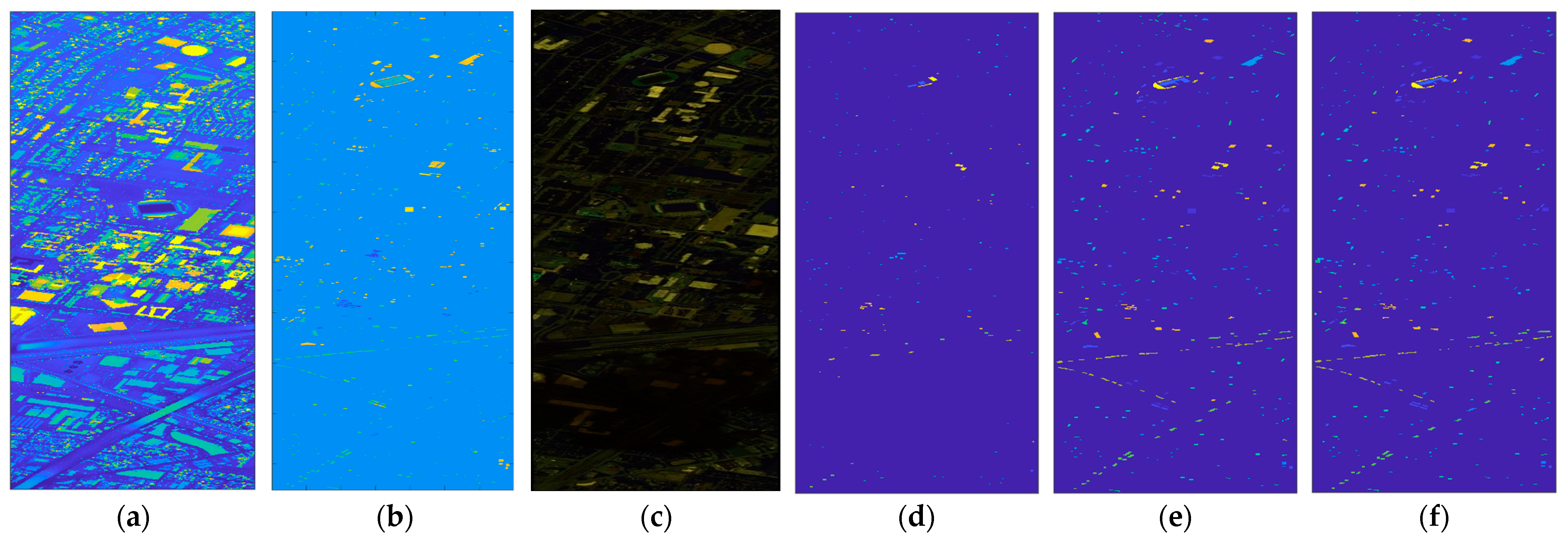
To validate the generalizability of the proposed method, the land cover classification experiments were conducted on the HSI-LiDAR MUUFL dataset. Our method was compared with traditional machine learning algorithms and state-of-the-art methods in the field of deep learning, including CCF, CoSpace, Co-CNN, FusAT-Net, ViT [57], S2FL, Spectral-Former, CCR-Net, and MFT. The specific results are illustrated in Figure 17, where (a) displays the three-band color composite for HSI spectral information, (b) shows the heatmap, (c) represents the LiDAR image, (d) shows the train ground-truth map, (e) shows the test ground-truth map, and (f) illustrates the classification results. The values of three universal indicators, namely OA, AA, and Kappa coefficient, are presented in Table 5, with the top outcomes being highlighted in bold. It is evident that our method outperforms the others in terms of OA (94.99%), AA (88.13%), and Kappa coefficient (0.9339). Our method surpasses other methods in five categories (grass-pure, water, buildings’-shadow, buildings, and sidewalk). Even in the remaining six categories, our method obtains commendable results. Therefore, statistically, our method exhibits superior performance compared to all other models. This shows that our method is general and universally applicable, and is thus a reliable model.

5. Discussion

5.1. Ablation Experiment

The ablation experiments were conducted on the QXS-SROPT dataset, the Houston 2013 dataset, and the MUUFL dataset to evaluate the proposed HGR correlation pooling fusion framework.
In the ablation experiments on QXS-SROPT datasets, the performance was observed when partially using the HGRPool, i.e., using the HGRPool for positive and negative samples or positive and zero samples, as well as when completely omitting it. The results of ablation experiments on the QXS-SROPT dataset are presented in Table 6. The proposed model demonstrates optimal performance in ship recognition experiments on the QXS-SROPT dataset when it incorporates all components, i.e., when fully utilizing the HGRPool. Meanwhile, there is a notable decline in ship recognition accuracy as the HGRPool component is partially employed or entirely excluded.
In the ablation experiments on the Houston 2013 and MUUFL datasets, the performance was observed when partially using HGRPool and completely omitting it. The results of ablation experiments on the Houston 2013 and MUUFL datasets are shown in Table 7. Similarly, the proposed model demonstrates optimal performance in land cover classification experiments on the Houston 2013 and MUUFL datasets when it incorporates all components, i.e., when fully utilizing the HGRPool. Due to partial use or complete exclusion of the HGRPool component, there is a significant decrease in land cover classification accuracy.

5.2. Analyzing the Effect of Experiments

The comparative experimental results confirm the precision and accuracy of our method. Compared with various advanced matching networks, this method not only achieves accurate and stable matching in ship recognition but also has particularly obvious advantages in land cover classification. By integrating a feature fusion method with an HGR correlation algorithm to separate information based on intrinsic correlation into different classification channels while maintaining information integrity, this model achieves information separation and maximizes the utilization of multimodal data, thereby improving the precision and accuracy of target recognition and classification.
From Table 6, it can be seen that the proposed model demonstrates optimal performance (with precision, recall, F1-score, and accuracy of 0.898, 0.908, 0.988, and 0.946, respectively) in ship recognition experiments on the QXS-SROPT dataset when it incorporated all components, i.e., fully using the HGRPool. There is a notable decline in ship recognition accuracy when the HGRPool component is partially used or entirely excluded. When partially using HGRPool (positive/negative sample), only recall (R) is still as high as 0.947. The results of accuracy, precision, and F1-score drop to 0.810, 0.849, and 0.895, respectively. The result of partially using HGRPool (positive/zero sample) is slightly worse than that of partially using HGRPool (positive/negative sample). Additionally, the result corresponding to without HGRPool is the worst, with accuracy, precision, recall, and F1-score being only 0.722, 0.803, 0.877, and 0.838, respectively.
Meanwhile, it can be deduced from Table 7 that there is a notable decline in land cover classification accuracy as the HGRPool component is partially employed or entirely excluded. The result of partially using HGRPool (positive/negative sample) in OA, AA, and Kappa drop to 90.81%, 91.46%, and 0.9013 on the Houston 2013 dataset and 93.79%, 85.07%, and 0.9180 on the MUUFL dataset. The result of partially using HGRPool (positive/zero sample) is slightly worse than that of partially using HGRPool (positive/negative sample). The result corresponding to without HGRPool is the worst, with OA, AA, and Kappa being only 89.64%, 90.26%, and 0.8851 on the Houston 2013 dataset and 92.72%, 80.94%, and 0.9040 on the MUUFL dataset. It can be concluded that the proposed HGR correlation pool fusion framework is effective and helps to improve accuracy.

6. Conclusions

The fusion of multimodal images has always been a research hotspot in the field of remote sensing. To address the issues of low recognition and classification accuracy and difficulty in integrating multimodal features in existing remote sensing data recognition and classification methods, this paper proposes a multimodal remote sensing data recognition and classification model based on a heatmap and HGR cross-correlation pooling fusion operation. Then, an HGR cross-correlation pooling fusion algorithm is proposed by combining the feature fusion method with the HGR cross-correlation algorithm. The model first calculates the statistical matrix through multimodal image pairs, extracts multimodal image features using convolutional layers, and then computes the heatmap from these features. Subsequently, by performing HGR cross-correlation pooling operations, the model can separate information with intrinsic relevance into respective classification channels, achieving dimensionality reduction of multimodal image features. In this approach, less feature data are used to represent the image area information of multimodal images while maintaining the original image information, thereby avoiding the problem of feature dimension explosion. Finally, point multiplication fusion is performed on the dimensionality-reduced feature samples, which are then input into the recognition and classification network for training to achieve recognition and classification of remote sensing data. This method maximizes the utilization of multimodal information, enhances the feature learning capability of multimodal images, improves the performance of specific interpretation tasks related to multimodal image fusion, and achieves classification and efficient utilization of information with different degrees of relevance. By conducting ship recognition experiments on the QXS-SROPT dataset and land cover classification experiments on the Houston 2013 and MUUFL datasets, it was fully verified that the proposed method outperforms other state-of-the-art remote sensing data recognition and classification methods. In future research, efforts will be made to further enhance recognition and classification accuracy and expand the application scope of this method to encompass more complex scenes and additional modalities. Further investigation will also be carried out of adaptive tuning of the parameters to achieve the best recognition and classification effects.

Author Contributions

Author Contributions: Conceptualization, H.Z. and S.-L.H.; methodology, H.Z., S.-L.H. and E.E.K.; validation, H.Z. and S.-L.H.; investigation, H.Z., S.-L.H. and E.E.K.; data curation, H.Z. and S.-L.H.; writing—original draft, H.Z.; writing—review and editing, S.-L.H. and E.E.K.; supervision, S.-L.H. and E.E.K.; funding acquisition, S.-L.H. and E.E.K. All authors have read and agreed to the published version of the manuscript.

Funding

This work was supported in part by the National Key R&D Program of China under Grant 2021 YFA0715202, Shenzhen Key Laboratory of Ubiquitous Data Enabling (Grant No. ZDSYS20220527171406015) and the Shenzhen Science and Technology Program under Grant KQTD20170810150821146 and Grant JCYJ20220530143002005.

Data Availability Statement

The Houston 2013 dataset used in this study is available at https://hyperspectral.ee.uh.edu/?page_id=1075 (accessed on 28 August 2023); the MUUFL dataset is available from https://github.com/GatorSense/MUUFLGulfport/ (accessed on 19 October 2023); the QXS-SAROPT dataset under open access license CCBY is available at https://github.com/yaoxu008/QXS-SAROPT (accessed on 27 June 2023).

Conflicts of Interest

The authors declare no conflicts of interest.

References

  1. Ghamisi, P.; Rasti, B.; Yokoya, N.; Wang, Q.; Hofle, B.; Bruzzone, L.; Bovolo, F.; Chi, M.; Anders, K.; Gloaguen, R.; et al. Multisource and multitem-poral data fusion in remote sensing: A comprehensive review of the state of the art. IEEE Geosci. Remote Sens. Mag. 2019, 7, 6–39. [Google Scholar] [CrossRef]
  2. Wu, X.; Hong, D.F.; Chanussot, J. Convolutional Neural Networks for Multimodal Remote Sensing Data Classification. IEEE Trans. Geosci. Remote Sens. 2022, 60, 1–10. [Google Scholar] [CrossRef]
  3. Hong, D.F.; Gao, L.R.; Yokoya, N.; Yao, J.; Chanussot, J.; Du, Q.; Zhang, B. More Diverse Means Better: Multimodal Deep Learning Meets Remote-Sensing Imagery Classification. IEEE Trans. Geosci. Remote Sens. 2020, 59, 4340–4354. [Google Scholar] [CrossRef]
  4. Li, X.; Lu, G.; Yan, J.; Zhang, Z. A survey of dimensional emotion prediction by multimodal cues. Acta Autom. Sin. 2018, 44, 2142–2159. [Google Scholar]
  5. Wang, C.; Li, Z.; Sarpong, B. Multimodal adaptive identity-recognition algorithm fused with gait perception. Big Data Min. Anal. 2021, 4, 10. [Google Scholar] [CrossRef]
  6. Zhou, W.J.; Jin, J.H.; Lei, J.S.; Hwang, J.N. CEGFNet: Common Extraction and Gate Fusion Network for Scene Parsing of Remote Sensing Images. IEEE Trans. Geosci. Remote Sens. 2021, 60, 1–10. [Google Scholar] [CrossRef]
  7. Asghar, M.; Khan, M.; Fawad; Amin, Y.; Rizwan, M.; Rahman, M.; Mirjavadi, S. EEG-Based multi-modal emotion recognition using bag of deep features: An optimal feature selection approach. Sensors 2019, 19, 5218. [Google Scholar] [CrossRef] [PubMed]
  8. Yang, R.; Wang, S.; Sun, Y.Z.; Zhang, H.; Liao, Y.; Gu, Y.; Hou, B.; Jiao, L.C. Multimodal Fusion Remote Sensing Image–Audio Retrieval. IEEE J. Sel. Top. Appl. Earth Obs. Remote Sens. 2022, 15, 6220–6235. [Google Scholar] [CrossRef]
  9. Li, H.; Wu, X. DenseFuse: A fusion approach to infrared and visible images. IEEE Trans. Image Process. 2019, 28, 2614–2623. [Google Scholar] [CrossRef]
  10. Yang, B.; Zhong, J.; Li, Y.; Chen, Z. Multi-Focus image fusion and super-resolution with convolutional neural network. Int. J. Wavelets Multiresolution Inf. Process. 2017, 15, 1750037. [Google Scholar] [CrossRef]
  11. Zhang, X. Benchmarking and comparing multi-exposure image fusion algorithms. Inf. Fusion. 2021, 74, 111–131. [Google Scholar] [CrossRef]
  12. Song, X.; Wu, X.; Li, H. MSDNet for medical image fusion. In Proceedings of the International Conference on Image and Graphic, Nanjing, China, 22–24 September 2019; pp. 278–288. [Google Scholar]
  13. Cao, X.F.; Gao, S.; Chen, L.C.; Wang, Y. Ship recognition method combined with image segmentation and deep learning feature extraction in video surveillance. Multimedia Tools Appl. 2020, 79, 9177–9192. [Google Scholar] [CrossRef]
  14. Wang, C.; Pei, J.; Luo, S.; Huo, W.; Huang, Y.; Zhang, Y.; Yang, J. SAR ship target recognition via multiscale feature attention and adaptive-weighed classifier. IEEE Geosci. Remote Sens. Lett. 2023, 20, 1–5. [Google Scholar] [CrossRef]
  15. Zhang, Z.L.; Zhang, T.; Liu, Z.Y.; Zhang, P.J.; Tu, S.S.; Li, Y.J.; Waqas, M. Fine-Grained ship image recognition based on BCNN with inception and AM-Softmax. CMC-Comput. Mater. Contin. 2022, 73, 1527–1539. [Google Scholar]
  16. Han, Y.Q.; Yang, X.Y.; Pu, T.; Peng, Z.M. Fine-Grained recognition for oriented ship against complex scenes in optical remote sensing images. IEEE Trans. Geosci. Remote Sens. 2022, 60, 1–18. [Google Scholar] [CrossRef]
  17. Liu, J.; Chen, H.; Wang, Y. Multi-Source remote sensing image fusion for ship target detection and recognition. Remote Sens. 2021, 13, 4852. [Google Scholar] [CrossRef]
  18. Cheng, G.; Xie, X.; Han, J.; Guo, L.; Xia, G.S. Remote sensing image scene classification meets deep learning: Challenges, methods, benchmarks, and opportunities. IEEE J. Sel. Top. Appl. Earth Obs. Remote Sens. 2020, 13, 3735–3756. [Google Scholar] [CrossRef]
  19. Zhu, X.; Tuia, D.; Mou, L.; Xia, G.; Zhan, L.; Xu, F.; Fraundorfer, F. Deep learning in remote sensing: A comprehensive review and list of resources. IEEE Geosci. Remote Sens. Mag. 2017, 5, 8–36. [Google Scholar] [CrossRef]
  20. Tsagkatakis, G.; Aidini, A.; Fotiadou, K.; Giannopoulos, M.; Pentari, A.; Tsakalides, P. Survey of deep-learning approaches for remote sensing observation enhancement. Sensors 2019, 19, 3929. [Google Scholar] [CrossRef]
  21. Gargees, R.S.; Scott, G.J. Deep Feature Clustering for Remote Sensing Imagery Land Cover Analysis. IEEE Geosci. Remote Sens. Lett. 2020, 17, 1386–1390. [Google Scholar] [CrossRef]
  22. Tan, C.; Ewe, H.; Chuah, H. Agricultural crop-type classification of multi-polarization SAR images using a hybrid entropy decomposition and support vector machine technique. Int. J. Remote Sens. 2011, 32, 7057–7071. [Google Scholar] [CrossRef]
  23. Xia, J.; Yokoya, N.; Iwasaki, A. Hyperspectral image classification with canonical correlation forests. IEEE Trans. Geosci. Remote Sens. 2016, 55, 421–431. [Google Scholar] [CrossRef]
  24. Jafarzadeh, H.; Mahdianpari, M.; Gill, E.; Moham-madimanesh, F.; Homayouni, S. Bagging and boosting ensemble classifiers for classification of multispectral, hyperspectral and PolSAR data: A comparative evaluation. Remote Sens. 2021, 13, 4405. [Google Scholar] [CrossRef]
  25. Li, X.; Lei, L.; Zhang, C.G.; Kuang, G.Y. Multimodal Semantic Consistency-Based Fusion Architecture Search for Land Cover Classification. IEEE Trans. Geosci. Remote Sens. 2022, 60, 1–14. [Google Scholar] [CrossRef]
  26. Cao, J.; Liu, K.; Zhuo, L.; Liu, L.; Zhu, Y.; Peng, L. Combining UAV-based hyperspectral and LiDAR data for mangrove species classification using the rotation forest algorithm. Int. J. Appl. Earth Obs. Geoinf. 2021, 102, 102414. [Google Scholar] [CrossRef]
  27. Yu, K.; Zheng, X.; Fang, B.; An, P.; Huang, X.; Luo, W.; Ding, J.F.; Wang, Z.; Ma, J. Multimodal Urban Remote Sensing Image Registration Via Roadcross Triangular Feature. IEEE J. Sel. Top. Appl. Earth Obs. Remote Sens. 2021, 14, 4441–4451. [Google Scholar] [CrossRef]
  28. Li, W.; Gao, Y.H.; Zhang, M.M.; Tao, R.; Du, Q. Asymmetric feature fusion network for hyperspectral and SAR image classification. IEEE Trans. Neural Netw. Learn. Syst. 2022, 34, 8057–8070. [Google Scholar] [CrossRef]
  29. Schmitt, M.; Zhu, X. Data fusion and remote sensing: An ever-growing relationship. IEEE Geosci. Remote Sens. Mag. 2016, 4, 6–23. [Google Scholar] [CrossRef]
  30. Zhang, Z.; Vosselman, G.; Gerke, M.; Persello, C.; Tuia, D.; Yang, M. Detecting Building Changes between Airborne Laser Scanning and Photogrammetric Data. Remote Sens. 2019, 11, 2417. [Google Scholar] [CrossRef]
  31. Schmitt, M.; Tupin, F.; Zhu, X. Fusion of SAR and optical remote sensing data–challenges and recent trends. In Proceedings of the IEEE International Geoscience and Remote Sensing Symposium (IGARSS), Fort Worth, TX, USA, 23–28 July 2017. [Google Scholar]
  32. Kulkarni, S.; Rege, P. Pixel level fusion recognition for SAR and optical images: A review. Inf. Fusion. 2020, 59, 13–29. [Google Scholar] [CrossRef]
  33. Rényi, A. On measures of dependence. Acta Math. Hung. 1959, 3, 441–451. [Google Scholar] [CrossRef]
  34. Huang, S.; Xu, X. On the sample complexity of HGR maximal correlation functions for large datasets. IEEE Trans. Inf. Theory 2021, 67, 1951–1980. [Google Scholar] [CrossRef]
  35. Liang, Y.; Ma, F.; Li, Y.; Huang, S. Person recognition with HGR maximal correlation on multimodal data. In Proceedings of the 25th International Conference on Pattern Recognition (ICPR), Milan, Italy, 25 August 2021. [Google Scholar]
  36. Wang, L.; Wu, J.; Huang, S.; Zheng, L.; Xu, X.; Zhang, L.; Huang, J. An efficient approach to informative feature extraction from multimodal data. In Proceedings of the AAAI Conference on Artificial Intelligence, Honolulu, HI, USA, 27 January–1 February 2019; Volume 33, pp. 5281–5288. [Google Scholar]
  37. Ma, F.; Li, Y.; Ni, S.; Huang, S.; Zhang, L. Data augmentation for audio-visual emotion recognition with an efficient multimodal conditional GAN. Appl. Sci.-Basel. 2022, 12, 527. [Google Scholar]
  38. Pande, S.; Banerjee, B. Self-Supervision assisted multimodal remote sensing image classification with coupled self-looping convolution networks. Neural Netw. 2023, 164, 1–20. [Google Scholar] [CrossRef] [PubMed]
  39. Poria, S.; Cambria, E.; Bajpai, R.; Hussain, A. A review of affective computing: From unimodal analysis to multimodal fusion. Inf. Fusion. 2017, 37, 98–125. [Google Scholar] [CrossRef]
  40. Pan, J.; He, Z.; Li, Z.; Liang, Y.; Qiu, L. A review of multimodal emotion recognition. CAAI Trans. Int. Syst. 2020, 15, 633–645. [Google Scholar]
  41. Pedergnana, M.; Marpu, P.; Dalla, M.; Benediktsson, J.; Bruzzone, L. Classification of remote sensing optical and LiDAR data using extended attribute profiles. IEEE J. Sel. Top. Signal Process. 2012, 6, 856–865. [Google Scholar] [CrossRef]
  42. Kim, Y.; Lee, H.; Provost, E. Deep learning for robust feature generation in audiovisual emotion recognition. In Proceedings of the IEEE International Conference on Acoustics, Speech and Signal Processing, Vancouver, BC, Canada, 26 May 2013. [Google Scholar]
  43. Kim, S.; Song, W.; Kim, S. Double weight-based SAR and infrared sensor fusion for automatic ground target recognition with deep learning. Remote Sens. 2018, 10, 72. [Google Scholar] [CrossRef]
  44. He, K.; Zhang, X.; Ren, S.; Sun, J. Deep residual learning for image recognition. In Proceedings of the 2016 IEEE Conference on Computer Vision and Pattern Recognition, Las Vegas, NV, USA, 26 January 2016. [Google Scholar]
  45. Huang, M.; Xu, Y.; Qian, L.; Shi, W.; Zhang, Y.; Bao, W.; Wang, N.; Liu, X.; Xiang, X. The QXS-SAROPT dataset for deep learning in SAR-optical data fusion. arXiv 2021, arXiv:2103.08259. [Google Scholar] [CrossRef]
  46. Debes, C.; Merentitis, A.; Heremans, R.; Hahn, J.; Frangiadakis, N.; Van Kasteren, T.; Liao, W.; Bellens, R.; Pizurica, A.; Gautama, S. Hyperspectral and LiDAR data fusion: Outcome of the 2013 GRSS data fusion contest. IEEE J. Sel. Top. Appl. Earth Obs. Remote Sens. 2014, 7, 2405–2418. [Google Scholar] [CrossRef]
  47. Gader, P.; Zare, A.; Close, R.; Aitken, J.; Tuell, G. MUUFL Gulfport Hyperspectral and Lidar Airborne Data Set; University of Florida: Gainesville, FL, USA, 2013. [Google Scholar]
  48. Du, X.; Zare, A. Technical Report: Scene Label Ground Truth Map for MUUFL Gulfport Data Set; University of Florida: Gainesville, FL, USA, 2017. [Google Scholar]
  49. Hong, D.; Hu, J.; Yao, J.; Chanussot, J.; Zhu, X. Multimodal remote sensing benchmark datasets for land cover classification with a shared and specific feature learning model. ISPRS J. Photogramm. Remote Sens. 2021, 178, 68–80. [Google Scholar] [CrossRef] [PubMed]
  50. Bao, W.; Huang, M.; Zhang, Y.; Xu, Y.; Liu, X.; Xiang, X. Boosting ship detection in SAR images with complementary pretraining techniques. IEEE J. Sel. Top. Appl. Earth Obs. Remote Sens. 2021, 14, 8941–8954. [Google Scholar] [CrossRef]
  51. Qian, L.; Liu, X.; Huang, M.; Xiang, X. Self-Supervised pre-training with bridge neural network for SAR-optical matching. Remote Sens. 2022, 14, 2749. [Google Scholar] [CrossRef]
  52. Roy, S.K.; Deria, A.; Hong, D.; Rasti, B.; Plaza, A.; Chanussot, J. Multimodal fusion transformer for remote sensing image classification. IEEE Trans. Geosci. Remote Sens. 2023, 61, 1–20. [Google Scholar] [CrossRef]
  53. Franco, A.; Oliveira, L. Convolutional covariance features: Conception, integration and performance in person re-identification. Pattern Recognit. 2017, 61, 593–609. [Google Scholar] [CrossRef]
  54. Hong, D.; Yokoya, N.; Chanussot, J.; Zhu, X. CoSpace: Common subspace learning from hyperspectral-multispectral correspondences. IEEE Trans. Geosci. Remote Sens. 2019, 57, 4349–4359. [Google Scholar] [CrossRef]
  55. Hang, R.; Li, Z.; Ghamisi, P.; Hong, D.; Xia, G.; Liu, Q. Classification of hyperspectral and LiDAR data using coupled CNNs. IEEE Trans. Geosci. Remote Sens. 2020, 58, 4939–4950. [Google Scholar] [CrossRef]
  56. Mohla, S.; Pande, S.; Banerjee, B.; Chaudhuri, S. FusAtNet: Dual attention based SpectroSpatial multimodal fusion network for hyperspectral and lidar classification. In Proceedings of the IEEE/CVF Conference on Computer Vision and Pattern Recognition Workshops (CVPRW), New Orleans, LA, USA, 14 June 2020. [Google Scholar]
  57. Khan, A.; Raufu, Z.; Sohail, A.; Khan, A.R.; Asif, A.; Farooq, U. A survey of the vision transformers and their CNN-transformer based variants. Artif. Intell. Rev. 2023, 56, 2917–2970. [Google Scholar] [CrossRef]
  58. Hong, D.; Han, Z.; Yao, J.; Gao, L.; Zhang, B.; Plaza, A.; Chanussot, J. SpectralFormer: Rethinking hyperspectral image classification with transformers. IEEE Trans. Geosci. Remote Sens. 2022, 60, 1–15. [Google Scholar] [CrossRef]
  59. Xu, G.; Jiang, X.; Zhou, Y.; Li, S.; Liu, X.; Lin, P. Robust land cover classification with multimodal knowledge distillation. IEEE Trans. Geosci. Remote Sens. 2024, 62, 1–16. [Google Scholar] [CrossRef]
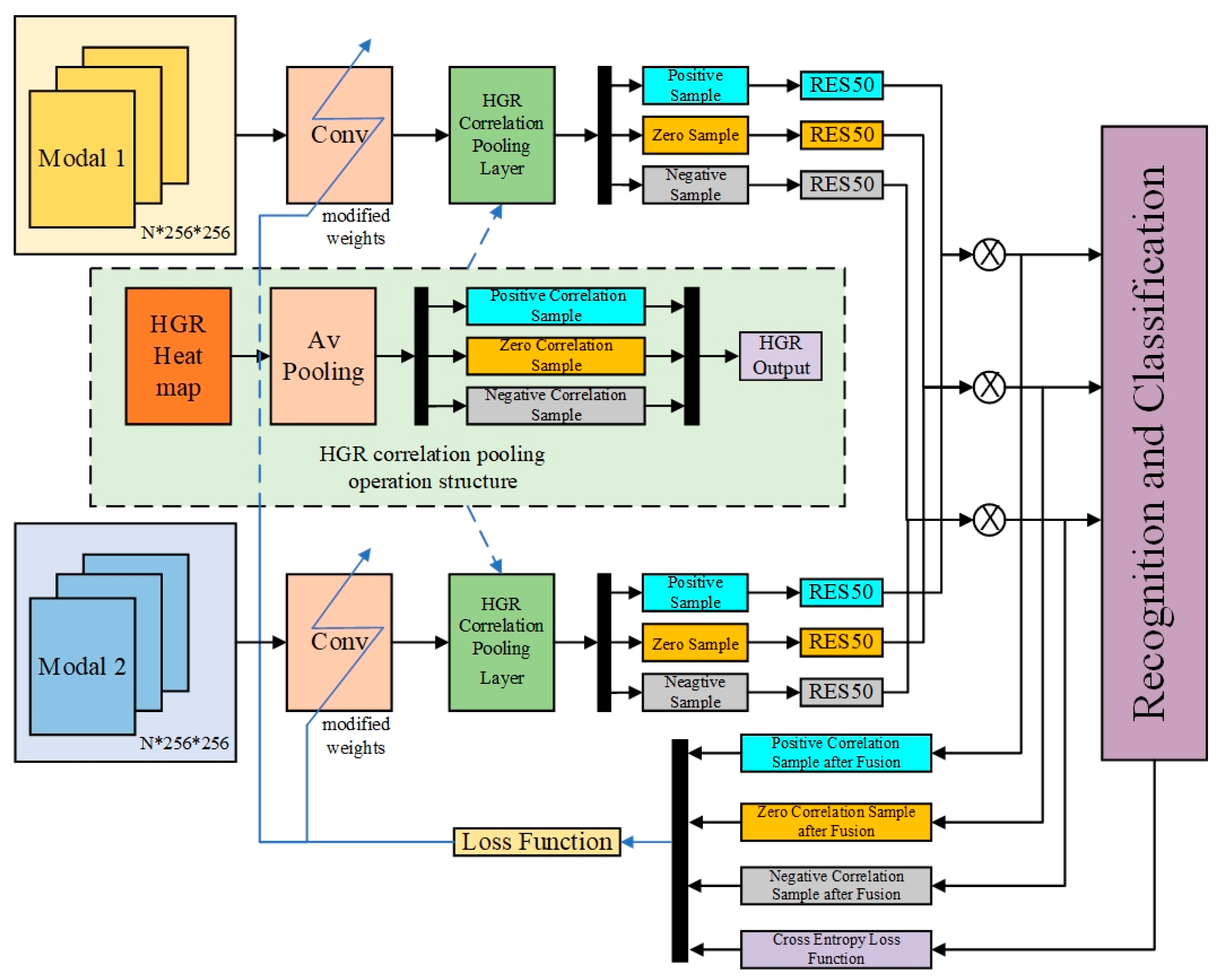
Figure 1. The overall framework of the proposed multimodal data fusion model.
Remotesensing 16 01708 g001
Figure 2. Statistical matrix calculation process.
Remotesensing 16 01708 g002
Figure 3. Heatmap calculation process.
Remotesensing 16 01708 g003
Figure 4. The calculation process of the HGR correlation sample matrix.
Remotesensing 16 01708 g004
Figure 5. HGR correlation pooling process.
Remotesensing 16 01708 g005
Figure 6. Sample division.
Remotesensing 16 01708 g006
Figure 7. Ship recognition experiment 1: (a) optical image; (b) heatmap; (c) SAR image; (d) ship recognition results.
Remotesensing 16 01708 g007
Figure 8. Ship recognition experiment 2: (a) optical image; (b) heatmap; (c) SAR image; (d) ship recognition results.
Remotesensing 16 01708 g008
Figure 9. Ship recognition experiment 3: (a) optical image; (b) heatmap; (c) SAR image; (d) ship recognition results.
Remotesensing 16 01708 g009
Figure 10. Optical information traceability experiment 1: (a) optical positive image; (b) optical negative image; (c) optical zero image; (d) optical original image.
Remotesensing 16 01708 g010
Figure 11. Optical information traceability experiment 2: (a) optical positive image; (b) optical negative image; (c) optical zero image; (d) optical original image.
Remotesensing 16 01708 g011
Figure 12. Optical information traceability experiment 3: (a) optical positive image; (b) optical negative image; (c) optical zero image; (d) optical original image.
Remotesensing 16 01708 g012
Figure 13. SAR information traceability experiment 1: (a) SAR positive image; (b) SAR negative image; (c) SAR zero image; (d) SAR original image.
Remotesensing 16 01708 g013
Figure 14. SAR information traceability experiment 2: (a) SAR positive image; (b) SAR negative image; (c) SAR zero image; (d) SAR original image.
Remotesensing 16 01708 g014
Figure 15. SAR information traceability experiment 3: (a) SAR positive image; (b) SAR negative image; (c) SAR zero image; (d) SAR original image.
Remotesensing 16 01708 g015
Figure 16. Houston 2013 dataset: (a) DSM obtained from LiDAR; (b) heatmap; (c) three-band color composite for HSI images (bands 32, 64, 128); (d) train ground-truth map; (e) test ground-truth map; (f) classification map.
Remotesensing 16 01708 g016
Figure 17. MUUFL dataset: (a) three-band color composite for HSI images (bands 16, 32, 64); (b) heatmap (c) LiDAR image; (d) train ground-truth map; (e) test ground-truth map; (f) classification map.
Remotesensing 16 01708 g017
Table 1. The Houston2013 dataset with 2832 training samples and 12,197 testing samples.
NoClass NameTraining SetTesting Set
1Healthy grass1981053
2Stressed grass1901064
3Synthetic grass192505
4Trees1881056
5Soil1861056
6Water182143
7Residential1961072
8Commercial1911053
9Road1931059
10Highway1911036
11Railway1811054
12Parking lot 11921041
13Parking lot 2184285
14Tennis court181247
15Running track187473
Total283212,197
Percentage18.84%81.16%
Table 2. The MUUFL Gulfport dataset with 2669 training samples and 51,018 testing samples.
NoClass NameTraining SetTesting Set
1Trees116622,080
2Grass-Pure2224048
3Grass-Groundsurface3566526
4Dirt-and-Sand861740
5Road-Materials3156372
6Water30436
7Buildings’-Shadow932140
8Buildings3025938
9Sidewalk741311
10Yellow-Curb9174
11ClothPanels16253
Total266951,018
Percentage4.97%95.03%
Table 3. Ship identification experimental results (best results are bolded).
ModelAccuracy (Acc)Precision (P)Recall (R)F1-Score
NP-BNN + ResNet500.8310.7500.9900.853
NP-BNN + Darknet530.8260.7610.9800.857
IP-BNN + ResNet500.8290.7480.9930.853
IP-BNN + Darknet530.8280.7460.9950.853
MoCo-BNN + ResNet500.8730.8080.9950.892
MoCo-BNN + Darknet530.8710.8090.9970.893
CCR-Net0.8540.8830.9630.894
MFT0.8760.8920.9800.934
HGRPool (ours)0.8980.9080.9880.946
Table 4. Comparison of various methods on the Houston 2013 dataset (best results are bolded).
ClassCCFCoSpaceCo-
CNN
FusAt-
Net
ViTS2FLSpectral-
Former
CCR-
Net
MFTDIMNetHGRPool
(Ours)
OA (%)83.4682.1487.2388.6985.0585.0786.1488.1589.1591.4792.23
AA (%)85.9584.5488.8290.2986.8386.1187.4889.8290.5692.4893.55
Kappa coefficient0.82140.80620.86190.87720.83840.83780.84970.87190.88220.90770.9157
Healthy grass83.1081.9683.196.8782.5980.0683.488382.7283.0083.00
Stressed grass83.9383.2784.8782.4282.3384.4995.5884.8785.0984.6898.87
Synthetic grass100.00100.0099.8100.0097.4398.0299.60100.0098.5599.01100.00
Trees92.4294.2292.4291.9592.9387.3199.1592.1495.9991.3898.58
Soil98.7799.3499.2497.9299.84100.0097.4499.8199.7899.6292.90
Water99.3099.3095.890.9184.1583.2295.1095.897.2095.10100.00
Residential84.4281.4495.2492.9187.8473.3288.9995.3486.3292.9198.50
Commercial52.9066.181.8689.4679.9374.8473.3181.3981.1687.2779.58
Road76.0269.9785.0882.0682.9478.3871.8684.1487.7688.0188.22
Highway67.1848.9461.166.6052.9383.3087.9363.2274.7193.8286.50
Railway84.4488.6183.8780.3680.9981.6980.3690.3293.7188.8091.46
Parking lot 192.8088.5791.2692.4191.0795.1070.7093.0896.1696.5497.50
Parking lot 276.4968.0788.7792.6387.8472.6371.2388.4292.5190.5390.88
Tennis court99.60100.0091.09100.00100.00100.0098.7996.36100.0096.76100.00
Running track97.8998.3198.7397.8999.6599.3798.7399.3786.8299.79100.00
Table 5. Comparison of various methods on the HSI-LiDAR MUUFL dataset (best results are bolded).
ClassCCFCoSpaceCo-
CNN
FusAt-
Net
ViTS2FLSpectral-
Former
CCR-
Net
MFTHGRPool
(Ours)
OA(%)88.2287.5590.9391.4892.1572.4988.2590.3994.3494.99
AA(%)71.7671.6377.1878.5878.5079.2368.4776.3181.4888.13
Kappa0.84410.83530.88220.88650.89560.65810.84400.86030.92510.9339
Trees96.5095.8998.9098.1097.8572.4097.3096.7897.9097.98
Grass-Pure77.1766.6578.6071.6676.0675.9769.3583.9992.1192.45
Grass-Groundsurface74.8085.2490.6687.6587.5854.7278.4884.1691.8089.86
Dirt-and-Sand91.9468.4590.6086.4292.0582.2082.6393.0591.5991.81
Road-Materials93.4594.5296.9095.0994.7371.2687.9191.3795.6095.13
Water95.0596.1075.9890.7382.0294.4258.7781.8888.1999.28
Buildings’-Shadow79.8284.9173.5474.2787.1177.3485.8776.5490.2793.25
Buildings98.2191.1996.6697.5597.6086.1995.6094.5897.2697.83
Sidewalk0.529.6964.9360.4457.8359.2153.5243.0261.3578.14
Yellow-Curb0.000.0019.4709.3931.9998.9108.4300.0017.4346.25
ClothPanels81.8995.2662.7693.0258.7298.8835.2994.7072.7987.45
Table 6. Ablation study by removing different modules on the QXS-SROPT dataset (best results are bolded).
MethodsAccuracy (Acc)Precision (P)Recall (R)F1-Score
Without HGRPool0.7220.8030.8770.838
Partially using HGRPool (positive/zero sample)0.7890.8340.9370.883
Partially using HGRPool (positive /negative sample)0.8100.8490.9470.895
HGRPool0.8980.9080.9880.946
Table 7. Ablation study by removing different modules on the Houston 2013 and MUUFL datasets (best results are bolded).
MethodsHouston 2013 DatasetMUUFL Dataset
OA (%)AA (%)KappaOA (%)AA (%)Kappa
Without HGRPool89.6490.260.885192.7280.940.9040
Partially using HGRPool (positive/zero sample)90.2091.050.893793.2484.410.9106
Partially using HGRPool (positive/negative sample)90.8191.460.901393.7985.070.9180
HGRPool92.2393.550.915794.9988.130.9339
Disclaimer/Publisher’s Note: The statements, opinions and data contained in all publications are solely those of the individual author(s) and contributor(s) and not of MDPI and/or the editor(s). MDPI and/or the editor(s) disclaim responsibility for any injury to people or property resulting from any ideas, methods, instructions or products referred to in the content.