Abstract
In this paper, we propose a global ionospheric total electron content (TEC) maps (GIM) prediction model based on deep learning methods that is both straightforward and practical, meeting the requirements of various applications. The proposed model utilizes an encoder-decoder structure with a Convolution Long Short-Term Memory (ConvLSTM) network and has a spatial resolution of 5° longitude and 2.5° latitude, with a time resolution of 1 h. We utilized the Center for Orbit Determination in Europe (CODE) GIM dataset for 18 years from 2002 to 2019, without requiring any other external input parameters, to train the ConvLSTM models for forecasting GIM 1, 2, and 3 days in advance. Using the CODE GIM data from 1 January 2020 to 31 December 2023 as the test dataset, the performance evaluation results show that the average root mean square errors (RMSE) for 1, 2 and 3 days of forecasts are 2.81 TECU, 3.16 TECU, and 3.41 TECU, respectively. These results show improved performance compared to the IRI-Plas model and CODE’s 1-day forecast product c1pg, and comparable to CODE’s 2-day forecast c2pg. The model’s predictions get worse as the intensity of the storm increases, and the prediction error of the model increases with the lead time.
1. Introduction
The ionosphere, extending from about 60 to 1000 km in altitude, is the ionized part of Earth’s upper atmosphere. There are many charged particles in the ionosphere, which have an important influence on the propagation of radio waves [1]. The total electron content (TEC) of the ionosphere represents the integrated total number of electrons within a column of one-meter squared cross-sectional area, also known as the columnar integral of the electron density. TEC is a very important parameter in the study of the ionosphere [2], which is proportional to the additional time delay of radio wave propagation caused by the ionosphere. Based on the study of TEC parameters, phenomena such as daily changes in the ionosphere and ionospheric disturbances are explored. From the perspective of the application, TEC prediction has a serious impact on the fields involving radio wave propagation and the electromagnetic environment, such as navigation, radar imaging, and short-wave communication. Therefore, the monitoring and prediction of the total electron content is an important research content of space weather [3].
In general, there are two types of TEC prediction models: the empirical models and the statistical models [4]. However, current statistical methods employed for regional TEC forecasting rely on relatively simple theoretical models. International Reference Ionosphere (IRI) [5,6] is one of the most widely used empirical models of the ionosphere, which was established by the International Union of Radio Sciences using a large amount of ground-related observation data and combining long-term accumulated ionospheric research results. The IRI-Plas model refers to the International Reference Ionosphere model extended to include the Plasmasphere. It presents comprehensive vertical analytical profiles of electron density, seamlessly conformed to IRI electron density profiles at the altitude corresponding to the upper half-peak density (400–600 km) and extending towards the plasmapause (up to 36,000 km) [7,8,9]. Typical empirical models also include the Klobuchar model [10] and the NeQuick model [11]; these two models help correct about 50% to 70% of the ionospheric delay in terms of root mean square (RMS) [11,12]. In 2011, A et al. presented a global ionospheric TEC model based on the empirical orthogonal function (EOF) analysis method [13]. This model is able to accurately reflect the majority of the variations and temporal-spatial distribution characteristics of the global ionospheric TEC. Also, in 2018, a data ingestion method was developed to incorporate TEC products from the Madrigal database into the NeQuick 2 model [14]. The NeQuick TEC, driven by the effective ionization parameter (Az) and modeled by EOF, shows an accuracy improvement of 10–15% compared to the standard ionospheric correction algorithm used in the Galileo navigation system. In 2022, Shubin proposed an approach to enhance the GTEC median global model of TEC under disturbed conditions, incorporating dynamic and aeronomic corrections based on spherical harmonic analysis of GIM-TEC Global Ionospheric Maps spanning 1996–2019, resulting in improved forecast accuracy compared to the IRI-Plas ionospheric reference model [15]. However, those models reflect regular variations of ionosphere TEC, while the instantaneous variations and perturbations cannot be well reflected. Therefore, many academics use statistical methods for forecasting. Among the existing approaches, auto-regressive moving average (ARIMA) [16,17], multiple linear regression model [18], support vector machine (SVM) [19], and artificial neural network (ANN) [20] are extensively used. In particular, Zhang et al. used an ARIMA model to predict global TEC. Results from numerical experiments show that during ionospheric quiet periods, the average relative prediction accuracy for a six-day period is up to 83.3% [17]. In 2020, Xia et al. were working on developing a regional forecast model for the ionospheric TEC over the China region using SVM algorithms. The results of the model’s predictions indicated that the RMSE ranges from 1.31 to 1.64 TECU, while the relative error (RE) varies from 10.73% to 15.86%, and the correlation coefficient falls within the range of 0.92–0.99 [19].
As early as 1997, Cander and Lamming began to use neural networks to analyze and predict nonlinear time series and use the multi-layer perceptron method to model different parameters of the ionosphere [21]. In the same year, Hochreiter and Schmidhuber developed long- and short-term memory neural networks [4]. Habarulema et al. developed neural networks for TEC prediction of the global positioning system over South Africa, and the results showed that neural networks (NNs) predict GPS TEC more accurately than the IRI at South African GPS locations [22]. Furthermore, a neural network-based prediction model with one input layer, two hidden layers, and one output layer was proposed in 2011. It was observed that ANNs extrapolate relatively well during quiet periods while the accuracy was low during geomagnetically disturbed conditions [23]. Recently, Song et al. proposed a genetic algorithm that improved the neural network to predict TEC in China, which has solved the problem that traditional neural networks tend to fall into local optimization, and the prediction error was about 5–8 TECU [24].
Deep learning is a specific type of machine learning. It is an upgrade on the basis of traditional artificial neural networks, which can use the training network to automatically extract the characteristics of data. This technique is considered to be a second-generation neural network [25]. In 2018, Yuan et al. established a 24-h ahead forecasting model for TEC at the Beijing station based on deep learning Recurrent Neural Network (RNN) and compared it with Back Propagation Neural Network (BPNN). The results showed that the RMSE of the disturbed ionosphere TEC predicted by the RNN model is lower than the BPNN model by 0.49~1.46 TECU [20]. The traditional recurrent neural network model may capture the time variations, but with the increase of input data, the influence of previous input values will gradually weaken or even disappear, and it fails to reflect long-term dependent information. In 2021, Xiong et al. proposed a novel extended encoder-decoder long short-term memory extended (ED-LSTME) neural network, and it was enhanced by considering solar flux and geomagnetic activity data, which obtained satisfactory results under geomagnetically disturbed conditions. In comparison to other statistical models, the ED-LSTME model exhibited greater performance, as evidenced by its lower root mean square error values of 12.09 TECU [26]. In 2022, Liu et al. apply ConvLSTM-based machine learning models to forecast global ionospheric TEC maps with up to 24 h of lead time. Results show that for the convLSTM model, the minimum RMSE values for quiet and storm time are 0.81 and 1.28 TECU, respectively, while the maximum RMSE values for quiet and storm time are 2.15 and 3.26 TECU, respectively [27]. Ren et al. developed an ionospheric long short-term memory network (Ion-LSTM) with multiple input parameters to predict the 1-day and 2-day global ionospheric TEC, which was evaluated with two solutions based on spherical harmonic coefficients (SHC) and vertical TEC (VTEC) prediction. The results show that both solutions perform well in accuracy and stability, and the RMSE of Ion-LSTM is 0.7 TECU lower than that of conventional methods under different solar and geomagnetic activities [28]. Furthermore, Ren et al. developed a new approach called the deep learning-based multi-model ensemble method (DLMEM) to forecast ionospheric TEC during geomagnetic storms. They utilized seven different features to model 170 geomagnetic storm events. The results of their study showed that the DLMEM model was able to reduce the RMSE by an average of 43.6% compared to their previously presented model, Ion-LSTM [29]. LSTM is a powerful tool for handling temporal variations due to its memory retention capabilities, but it has limitations when dealing with problems that have both temporal and spatial characteristics. To address this, the paper introduces the convolution operation, which can effectively extract the spatial features of the data. By combining the temporal feature extraction ability of LSTM with the spatial feature extraction ability of convolution, the model can more effectively extract spatiotemporal features.
Most of the research mentioned above incorporates solar and geomagnetic indices as training data. Since the ionosphere is closely related to solar and geomagnetic activities, this approach often leads to better forecasting results. However, in specific instances such as equipment maintenance, network failures, holiday periods, etc., the timely acquisition of geomagnetic and solar indices might pose limitations. These conditions may limit the use of the model and fail to meet the requirements of operational forecasting [30,31,32,33]. Real-time collection of monitoring data emerges as a crucial factor in the transition from Space Weather Research to Operations (R2O) [34,35,36]. The forecast products of CODE, such as c1pg, which is produced based on the extrapolation of spherical harmonic (SH) coefficients [27], reducing reliance on external parameters. These products release regular global ionospheric TEC map forecast products accurately every day, which can be used by the majority of navigation and positioning users. This paper addresses the operational forecasting requirements for ionospheric TEC maps, employing the ConvLSTM model to develop a predictive model for global ionospheric TEC maps, capable of providing forecast products for ionospheric TEC maps for the next 1, 2, and 3 days.
To improve the accuracy of predicting ionospheric TEC, this paper utilizes a ConvLSTM neural network. This deep learning technique enables the prediction of ionospheric TEC maps with a time accuracy of 1 h, providing insight into the spatiotemporal variations of global TEC. In this study, we utilized an encoder-decoder structured neural network to implement the ConvLSTM architecture. The convolutional layers and pooling layers for feature extraction and dimensionality reduction are efficient for speeding up network training and reducing data size, while the middle layer uses a convolution long short-term memory network to obtain the time series prediction [37]. The data set used in this paper is based on GIM provided by CODE from 2002 to 2022. The aim of this work is to predict the GIM 1, 2, and 3 days in advance. In particular, the performance of this model compared to other model predictions and with different geomagnetic storm levels on the model are also discussed.
2. Data and Methods
This section presents the source, format, and resolution of data we used in this study. Then, the principle of the ConvLSTM network and the data preprocessing were introduced. Furthermore, we calculated the RMSE, mean relative deviation (MRD in %), and mean absolute error (MAE) as evaluation metrics for the prediction performance of the proposed model.
2.1. Data Description
The ionospheric TEC dataset is a global ionospheric GIM-TEC data generated in the standard Ionosphere map exchange format (IONEX) file format provided by the International GNSS Service (IGS). IGS has many ionosphere associate analysis centers that provide global ionospheric TEC map operational forecast products, such as CODE, Jet Propulsion Laboratory (JPL), and European Space Agency (ESA). This paper utilizes GIM data from CODE for the purpose of research. Since 19 October 2014, the time resolution of CODE-TEC data has changed from 2 h to 1 h. The longitude ranges from 180° west to 180° east, and the latitude ranges from 87.5° south to 87.5° north. The spatial resolution is 5° longitude and 2.5° latitude.
The time range of the data set is from 1 January 2002 to 31 December 2023, and the data of each day constitutes a file. The time resolution of data from 1 January 2002 to 18 October 2014 has been changed to 1 h through interpolation. According to the information above, the scale of the grid points of the GIM is 71 × 73. In addition, we can combine the TEC map data of one day, which is 24 TEC maps, as the input of a single sample, and the output of the sample is the 24 TEC maps of the next day. Then, a five-dimensional tensor can be derived, and its dimensions are (number, 24, 71, 73, 1). “Number” represents the total amount of samples in the data set, as an example, “24” represents that each sample contains 24 h which means 24 TEC maps, “71” and “73” are the dimensions of the TEC map at each hour, “1” represents the number of color channels for maps, because the TEC for each latitude and longitude is a one-dimensional value.
The CODE TEC data used in this study are from 1 January 2002 to 31 December 2019, which are divided into training (95%) sets and validation (5%) sets. Data from 1 January 2020 to 31 December 2023 were used for testing sets.
2.2. ConvLSTM Network
This paper uses deep learning to predict the TEC map of the global ionosphere. A classic encoder-decoder framework was used to build a deep neural network. This framework is also known as a self-encoding decoder; it mainly converts the input vector into an intermediate vector with lower dimensions through the encoder, then uses the decoder to convert this intermediate variable into an output variable [38]. To process ionospheric TEC data with both temporal and spatial features, the ConvLSTM model was used to predict GIM.
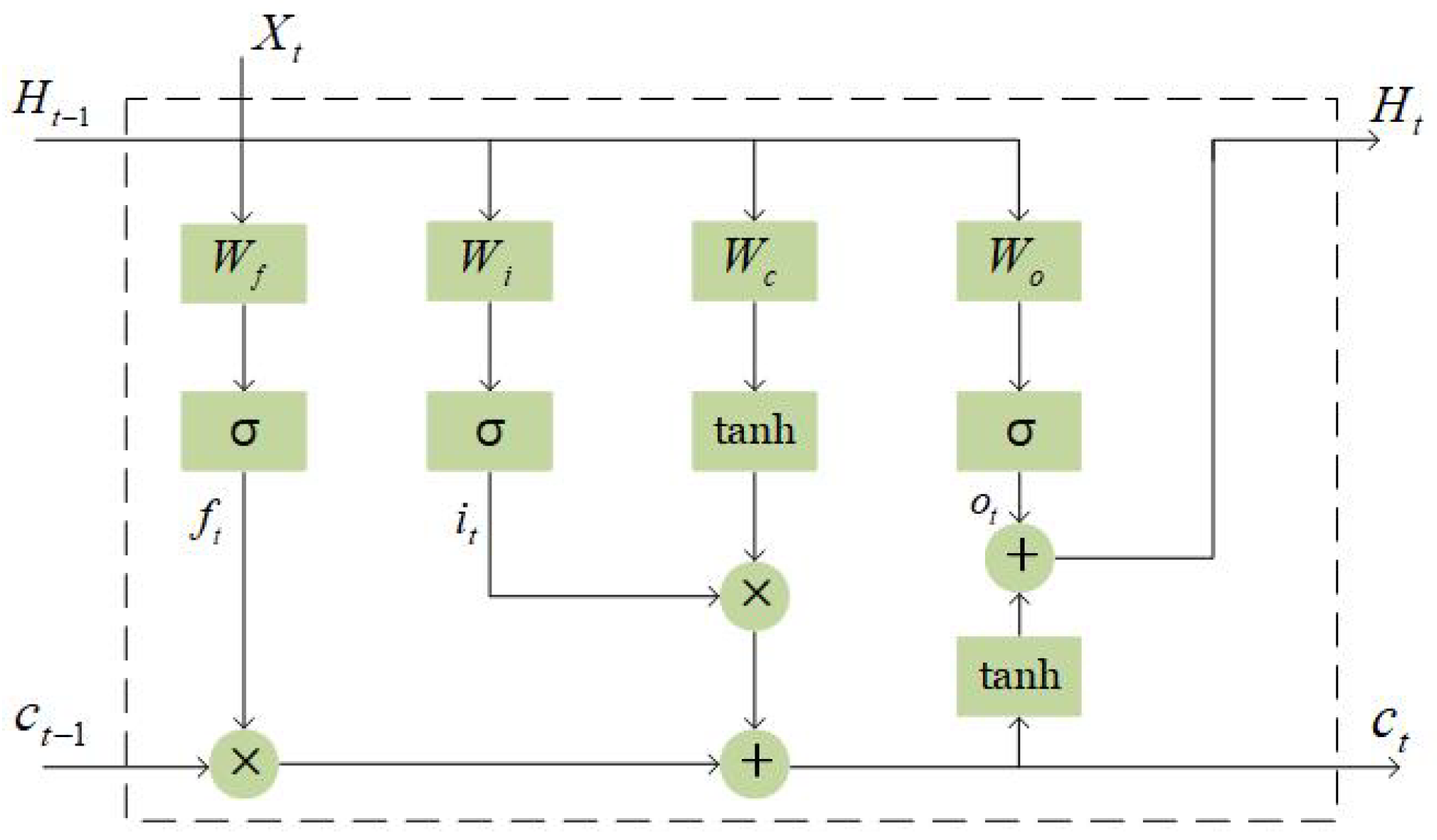
Figure 1 shows the inner structure of the ConvLSTM network at time point . The ConvLSTM network uses input gates , output gates , forget gates , and the same memory cells as the hidden state to record additional information. The input of all gates is composed of the input at the current time t and the hidden state at the time point . The key equations of ConvLSTM are shown as:
where represents the weights and represents bias coefficients. represents the final output at time point , which will be input at time point along with cell state . Here, ‘⊗’ denotes the convolution operator, and ‘*’ denotes the Hadamard product.
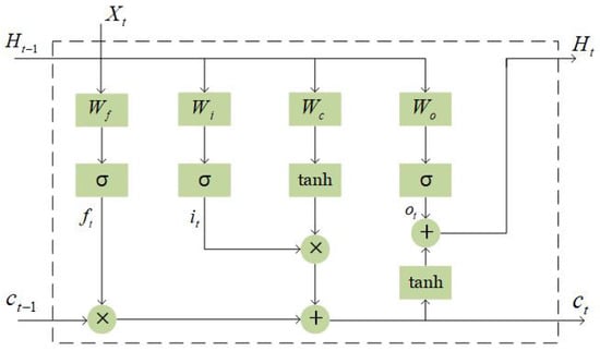
Figure 1.
Inner structure of the convolution-optimized long and short-term memory network at time point .
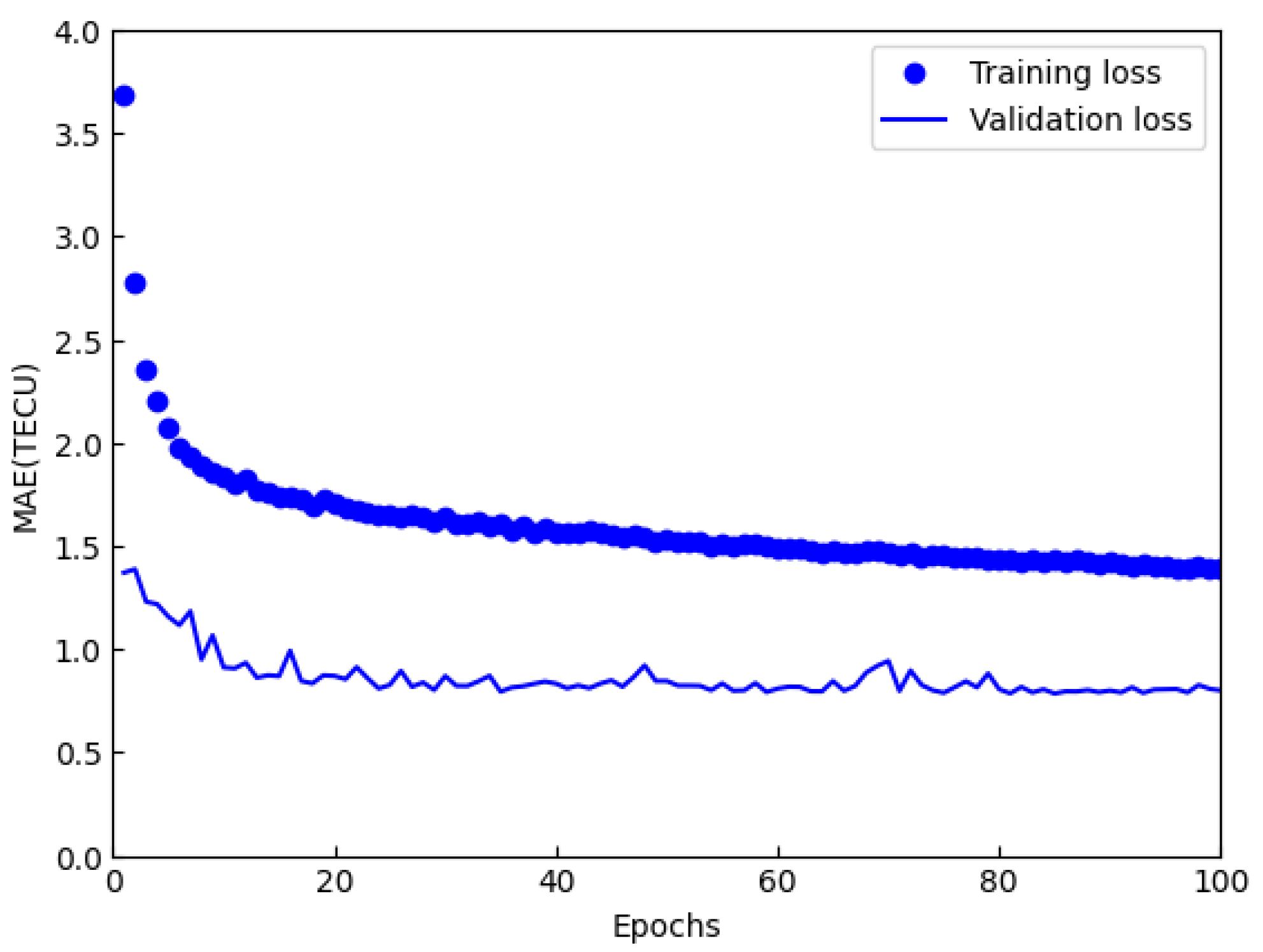
In this study, the Python 3.9.16 programming language was utilized to write deep learning code based on the Keras library. The neural network was constructed using this framework and trained on a server equipped with NVIDIA A100 GPUs and 83.5 GB of RAM. The whole neural network structure can be divided into three parts. The first part is the encoder, which is the combination of the convolutional layer and the pooling layer. This design can effectively extract the spatial key features of the input GIM, which means fewer network parameters and a faster training process. The second part consists of a ConvLSTM network, which can extract the time series features of TEC maps, and a batch normalization layer used to prevent overfitting and normalize data. The last part is the decoder, which consists of an upsampling layer and a convolutional layer corresponding to the encoder. The input is 24 GIMs with a time accuracy of 1 h from 00:00 UT to 23:00 UT. The output is the same GIM on the next day. The activation function of the convolutional layer is the Exponential Linear Unit (Elu) function. The loss function was MAE, and the optimizer used the improved Adamax algorithm that adaptively adjusts the learning rate [39]. The batch size was 32, while the number of training rounds was set to 100. Deep learning code is written using Python and the high-level abstraction of the Keras library (with TensorFlow as the backend) to construct the neural network. By continuously adjusting the kernel size and number of filters for each layer, a well-trained model is obtained. Figure 2 shows the change curve of the loss function during the training process. It can be observed that both the validation set error and training set error gradually decrease with the increase in training epochs and eventually stabilize.
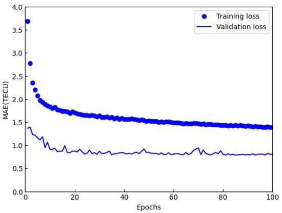
Figure 2.
Variation curve of training set loss and validation set loss error with epoch.
2.3. Evaluation Metrics
To quantify the prediction performance of the ConvLSTM model, the RMSE, MRD and MAE were estimated, the formula is as follows:
where is the number of TEC bins, is the predicted TEC values and is the real values.
3. Results
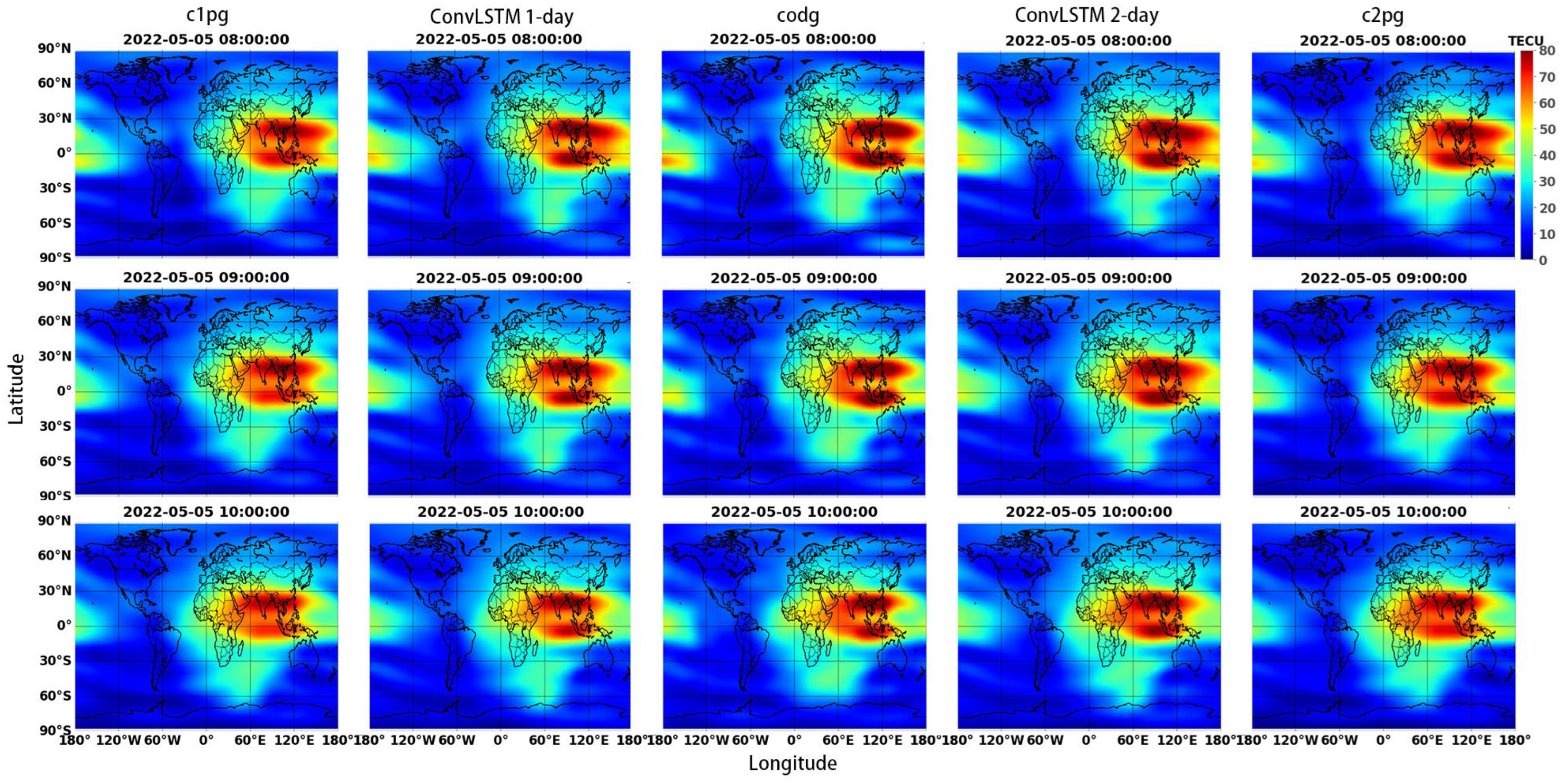
In this section, we presented the results by comparing the ConvLSTM predictions with c1pg, c2pg, IRI-Plas, and CODE data, which serves as the ground truth from the CODE analysis center, to assess the accuracy of the ConvLSTM model. The c1pg and c2pg in Figure 3 are 1-day and 2-day predicted global TEC maps released by CODE which is produced based on the extrapolation of spherical harmonic (SH) coefficients [40]. The IRI-Plas model is one of the best-known empirical models of the ionosphere and plasmasphere. The model used in this paper is the IRI-Plas 2020 model.
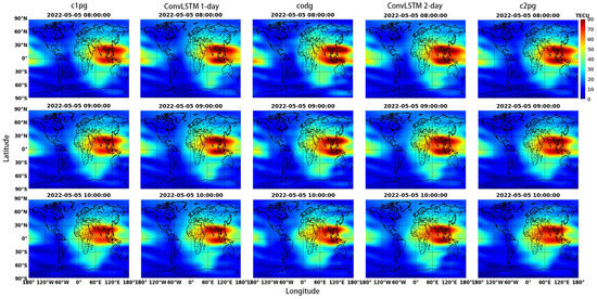
Figure 3.
An example of predicted global TEC maps at 1 h interval during geomagnetic quiet day. The first and last column represents the 1-day and 2-day predicted global ionospheric TEC maps released by CODE. The second and fourth column represents the 1-day and 2-day predicted TEC maps from ConvLSTM model. And the middle column codg represents the ground truth provided by CODE.
Figure 3 shows the 1 h interval global TEC maps predicted by c1pg, c2pg, and ConvLSTM models, along with the ground truth during geomagnetic quiet day. The figures showed that all TEC maps from c1pg, c2pg, and ConvLSTM are well in agreement with the ground truth. In addition, the ConvLSTM is closer to the truth than c1pg and c2pg maps where TEC is enhanced on the day side. For example, the TEC enhancement showed around 80°E–120°E longitude, 0°–20°S latitude is well reproduced in the ConvLSTM, while the c1pg and c2pg cannot reflect it. By using Formula (7) for calculation, we obtained the RMSE of c1pg on 5 May 2022 as 3.32 TECU, the RMSE of c2pg is 3.63 TECU, while the RMSE of ConvLSTM 1-day is 3.03 TECU, the RMSE of ConvLSTM 2-day is 3.06 TECU. This shows that the error between the predicted results of ConvLSTM and the actual TEC data is better than that of c1pg and c2pg. As expected, the 1-day predicted TEC maps of both ConvLSTM and those released by CODE are closer to the ground truth than the 2-day predicted.
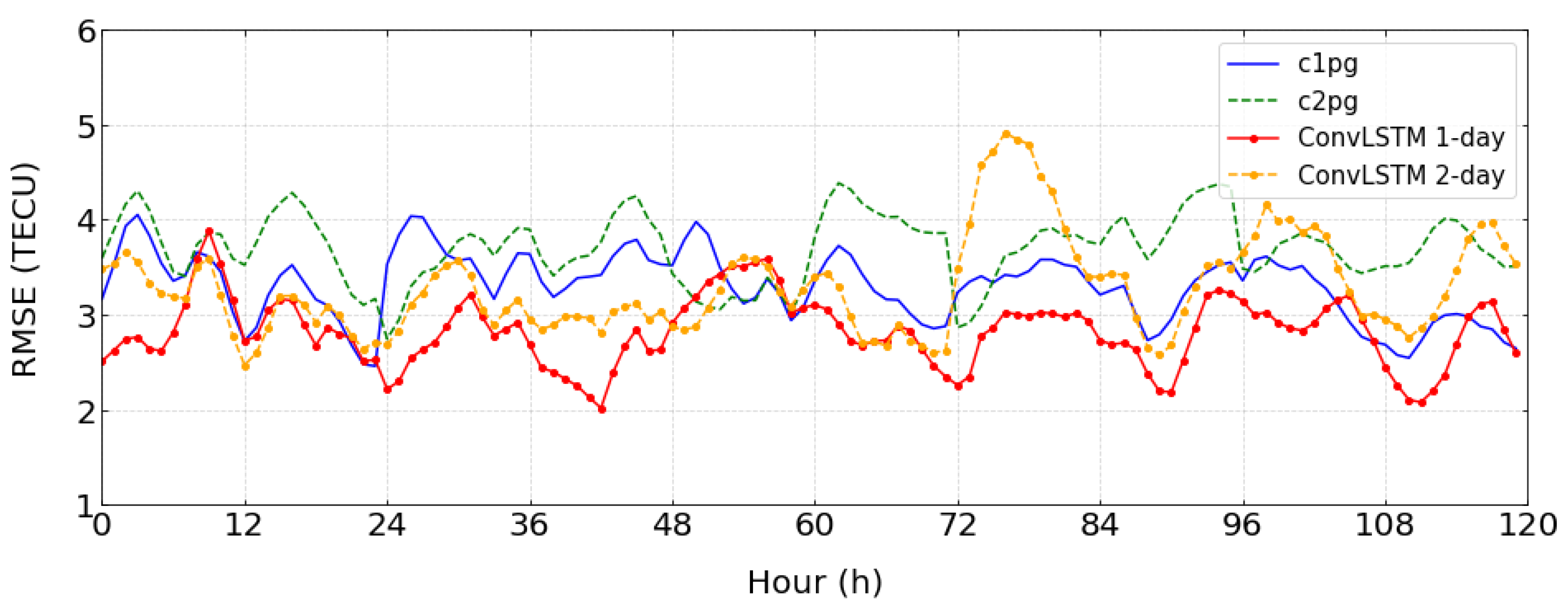
Figure 4 shows a comparison of hourly RMSE error between global ionospheric TEC maps released by CODE and ConvLSTM during some geomagnetic quiet days. Whereas the 95% confidence interval for c1pg is ±0.06, for c2pg it is ±0.07, for ConvLSTM 1-day model is ±0.06, and for ConvLSTM 2-day model is ±0.09. The results show that our ConvLSTM 1-day model outperforms the c1pg model, as it has a smaller RMSE. Similarly, the c1pg model has a smaller RMSE than the c2pg model, indicating that our ConvLSTM 1-day model has a better prediction ability. Moreover, our ConvLSTM 2-day model performs similarly to the c2pg model in terms of performance. Furthermore, the RMSE of ConvLSTM shows an obvious decline about every 12 h during geomagnetic quiet days.
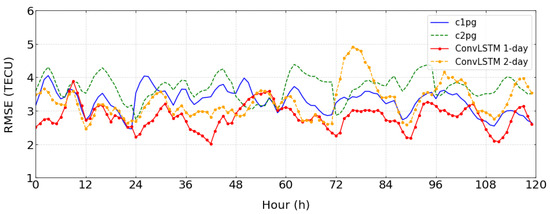
Figure 4.
The plot is hourly RMSE error from 1-day (red line) and 2-day (orange dotted line) predicted TEC maps from ConvLSTM model and c1pg (blue line), c2pg (green dotted line) from 3 May to 7 May 2022 (geomagnetic quiet days).
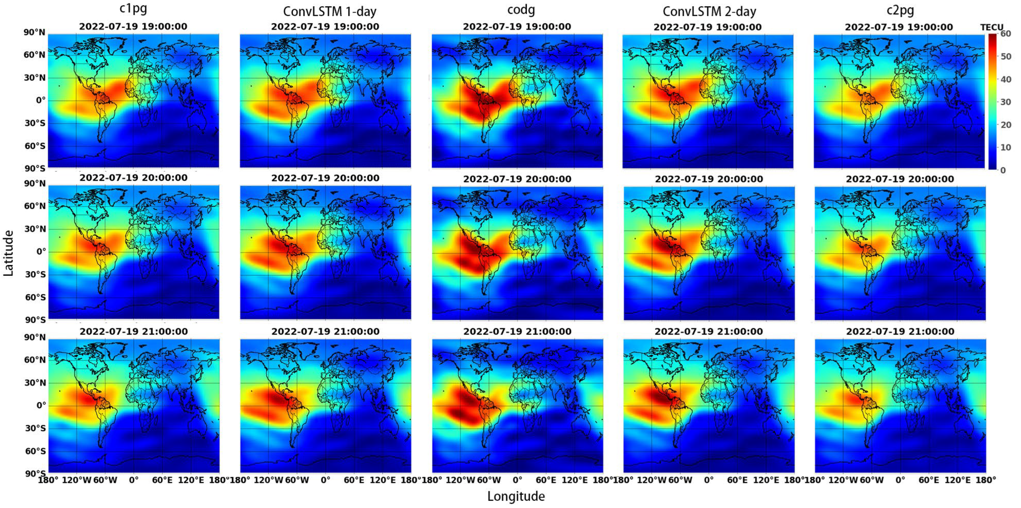
Figure 5 displays a comparison of 1-h interval TEC maps during the main phase of a geomagnetic storm event from UT 19:00 to UT 21:00, 19 July 2022, during which the Dst index declines to −62 nT. The figure shows the ConvLSTM prediction along with the global ionospheric TEC maps released by CODE and the ground truth. The plots reveal that the maps predicted by the ConvLSTM model for 1-day and 2-day intervals are more accurate than those generated by c1pg and c2pg, as they exhibit closer proximity to the ground truth. The TEC enhancement showed a latitude near 0°N–30°N on the day side, which is captured by the ConvLSTM model, while c1pg and c2pg fail to reflect it. By using Formula (7) for calculation, we obtained the RMSE of c1pg on 19 July 2022 as 4.4 TECU, the RMSE of c2pg is 4.22 TECU, while the RMSE of ConvLSTM 1-day is 3.41 TECU, the RMSE of ConvLSTM 2-day is 3.98 TECU. Moreover, the prediction results from ConvLSTM in Figure 2 are more consistent with those from the truth compared with Figure 4, indicating the prediction capability performance of c1pg, c2pg, and ConvLSTM decrease as the storm level increases.

Figure 5.
An example of predicted global TEC maps at 1 h interval during geomagnetic storm event from UT 19:00 to UT 21:00, 19 July 2022, where the Dst index declines to −62 nT. The first and last column represents the 1-day and 2-day predicted global ionospheric TEC maps released by CODE. The second and fourth column represents the 1-day and 2-day predicted TEC maps from ConvLSTM model. The middle column represents the ground truth provided by CODE.
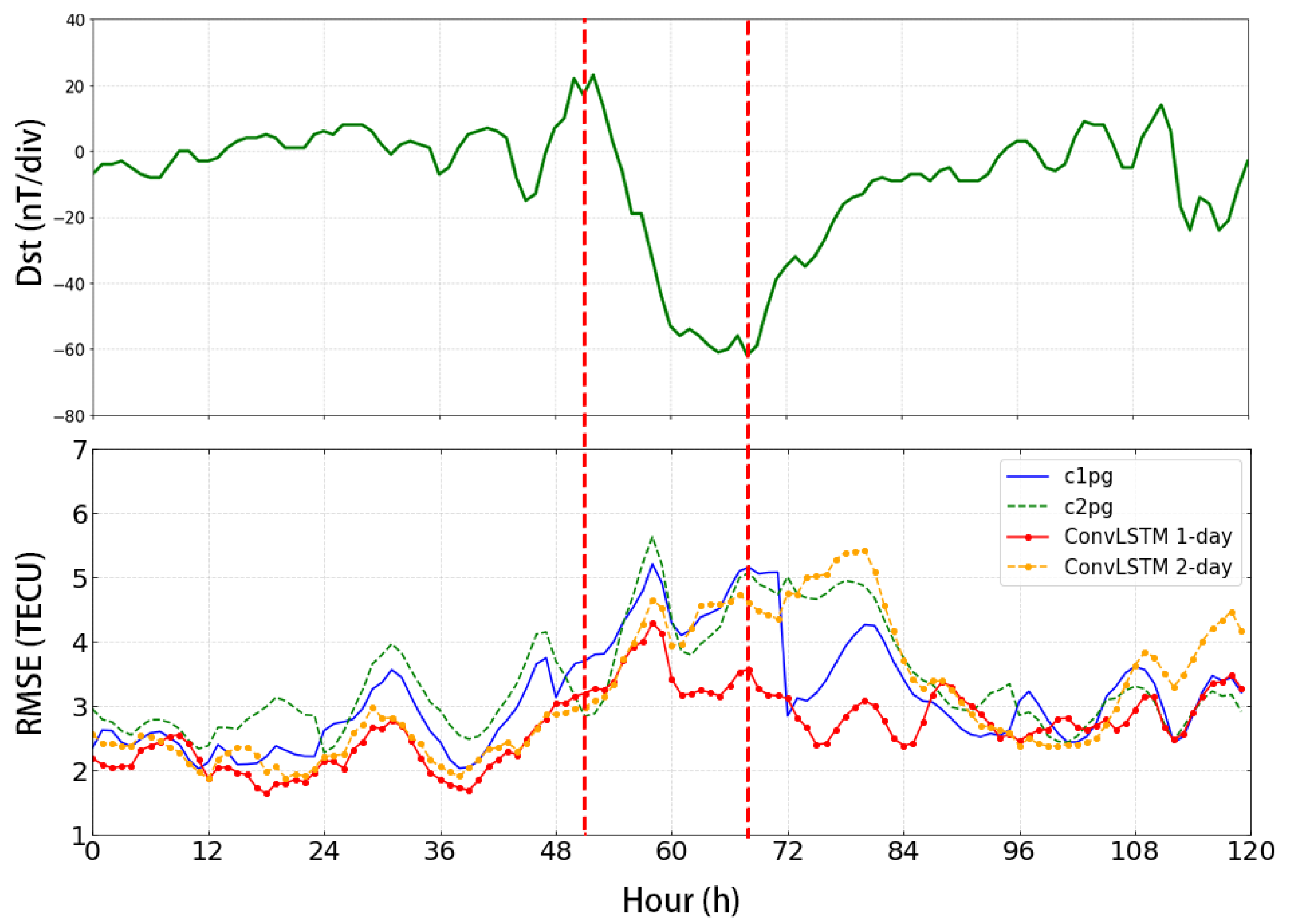
Figure 6 shows the Dst variations during 17–21 July 2022, where the minimum reaches −62 nT, comparing the hourly RMSE error from ConvLSTM 1-day and c1pg for the storm time. The 95% confidence interval in the figure for c1pg is ±0.14; for c2pg it is ±0.16; for ConvLSTM 1-day model is ±0.1, and for ConvLSTM 2-day model is ±0.17. It can be seen that the presented results demonstrate a high level of statistical credibility. In general, the ConvLSTM model shows smaller RMSE than c1pg during the main phase of the storm events. The performance of ConvLSTM prediction is better than c1pg, especially during the main phase of the storm event, indicating an improved prediction capability for the storm time. However, the performance of the 2-day prediction of both the c2pg and ConvLSTM model during the main phase of a geomagnetic storm event is not very satisfactory.
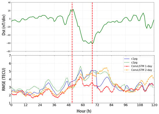
Figure 6.
The first plot is Dst (green line) variations from 17 July to 21 July 2022, and the main phase of geomagnetic storm event (between the two red dotted lines). The second plot is hourly RMSE error from 1-day (red line) and 2-day (orange dotted line) predicted TEC maps of ConvLSTM, c1pg (blue line) and c2pg (green dotted line).
Table 1 shows the classification of geomagnetic storm levels [41,42,43,44,45]. Table 2 displays a quantitative estimate of the RMSE, MRD, MAE, and their confidence intervals (95%) for models during the main phase of geomagnetic storm events of different levels. The result is calculated by Formulas (7)–(9). As the level of geomagnetic storm increases, the predictive performance of the model gradually becomes less satisfactory. The largest errors are obtained in the IRI-Plas model for the intense storm events. It can be observed that the performance of the ConvLSTM 1-day model is better than that of c1pg, while the ConvLSTM 2-day is roughly equivalent to c2pg. By calculating the 95% confidence interval, the presented results exhibit a higher statistical credibility.

Table 1.
Classification of Storms.

Table 2.
Root mean square error RMSE (TECU), mean relative error MRD (%), mean absolute error MAE (TECU), and their confidence intervals (95%) of the model under different levels of magnetic storm events.
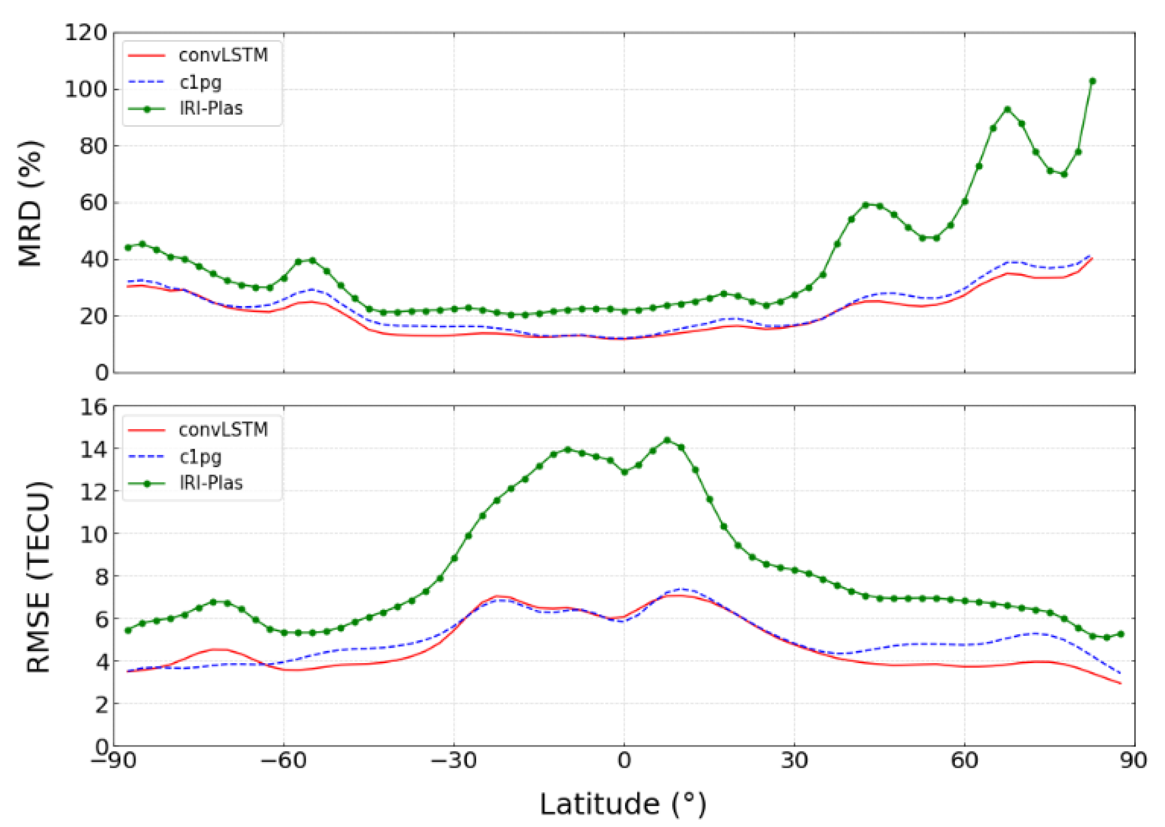
Figure 7 illustrates the variation of RMSE and MRD in the test dataset for the year 2023 as latitude changes. The 95% confidence interval of the RMSE in the figure for c1pg is ±0.025, for the ConvLSTM 1-day model, it is ±0.024, and for the IRI-Plas model, it is ±0.044. Notably, the ConvLSTM model demonstrates the lowest error. It is evident that the ConvLSTM model outperforms c1pg notably in mid-latitudes. All three models exhibit pronounced latitude-dependent RMSE errors, a phenomenon that might be linked to Equatorial Ionization Anomaly (EIA). In high-latitude regions, GIM-TEC values are often very small or even zero, resulting in larger MRD values.
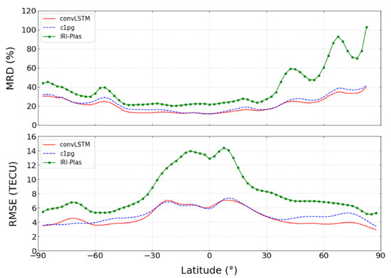
Figure 7.
The variation of RMSE MRD in the test dataset for the year 2023 as latitude changes.
Figure 8 displays the temporal variations of RMSE for different forecast days, revealing a periodic change. The 95% confidence interval in the figure for c1pg is ±0.023; for c2pg it is ±0.024; for ConvLSTM 1-day model is ±0.022; for ConvLSTM 2-day model is ±0.025, for ConvLSTM 3-day model is ±0.027, and for IRI-Plas model is ±0.033. In the performance of the whole year, the RMSE of ConvLSTM 1-day is the smallest, the prediction performance of ConvLSTM 1-day is better than c1pg, and the prediction performance is the best. Additionally, as the number of days being forecasted increases, the RMSE value also tends to increase, indicating a decrease in the predictive accuracy of the ConvLSTM model over longer forecast horizons. The prediction effect of the model is related to the season, and the RMSE value in the northern hemisphere summer is smaller than that in spring, autumn, and winter. It is well known that the ionosphere is more stable in summer due to longer periods of solar irradiance. In other seasons, however, dynamical processes become significant, leading to poor results for any prediction method based on previous observations.

Figure 8.
The RMSE values averaged over each month of TEC prediction by ConvLSTM 1-day, 2-day, 3-day compared with c1pg, c2pg and IRI-Plas models in 2022.
The trained model was utilized to analyze the ionospheric TEC prediction error 1 day in advance, using the entire test set. Formula (7) was applied to calculate the RMSE of each prediction. The resulting distribution histogram of the RMSE is displayed in Figure 9. Based on the histogram shown in Figure 9, the trained model exhibited a mean RMSE value of 3.17 TECU and a standard deviation of 0.86 TECU in 2022, indicating a high level of stability in its predictions. Furthermore, the mean RMSE values for the ConvLSTM 2-day and 3-day predictions were 3.16 TECU and 3.41 TECU, respectively.
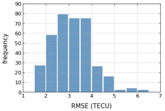
Figure 9.
The histogram of 1-day prediction error in 2022. (μ = 3.17, σ = 0.86).
4. Conclusions
Currently, the solar activity index and geomagnetic index are mostly used as input layer characteristic parameters in the ionospheric TEC map forecast modeling studies, but these parameters often need to be acquired by actual measurements, and their accuracy and timeliness directly affect the performance of the model, which is not conducive to the engineering development and application of the model. In this paper, a ConvLSTM model combined with CNN was proposed to predict GIM. The CODE GIM from 2002 to 2019 was used to train (95%) and validate (5%) the model, and data from 1 January 2020 to 31 December 2023 were used for testing sets to forecast TEC maps 1, 2, and 3 days in advance. The model was compared to IRI-Plas, c1pg, and c2pg, and the results indicated that our model provided more accurate predictions, particularly during geomagnetic storm periods. Based on the comparison of our model with IRI-Plas, c1pg and c2pg on the test set, as well as its performance under different magnetic storm conditions, the following conclusions were drawn:
- The mean RMSE of 1-day prediction in 2022 is 3.17 TECU, and the standard deviation of the error is 0.86 TECU, which shows a relatively stable performance during the geomagnetic quiet and small magnetic storms. The mean RMSE of ConvLSTM 1-day prediction is 2.81 TECU, ConvLSTM 2-day is 3.16 TECU, while the mean RMSE of 3-day prediction is 3.41 TECU;
- Our findings suggest that the ConvLSTM 1-day model outperforms c1pg in situations characterized by geomagnetic quietness and small magnetic storm conditions. However, the performance of our ConvLSTM 2-day model is similar to that of c2pg. Model predictions get worse as the intensity of the storm increases;
- The prediction RMSE of the model gradually increases with the increase of the prediction date.
- In conclusion, the proposed global ionospheric TEC forecasting model in this paper is simple, practical, and has a relatively high forecast accuracy. By only inputting the GIM of the current day, it can forecast the GIM for the next 1, 2, and 3 days, which is convenient for engineering applications. Providing timely, precise, and dependable ionospheric TEC data, along with error correction information, is crucial for scientific research and engineering applications. These datasets find utility in various fields, including satellite navigation, radar imaging, mitigation of radiocommunication issues, aviation purposes, shortwave communication, and more. Geomagnetic perturbations have an important impact on the ionosphere, but forecasting magnetic storms is still a challenging task [46]. With increasing geomagnetic activity, the impacts of energetic particle precipitation on electron production in the ionosphere become more significant [47,48]. Therefore, we did not include geomagnetic indices in our training mainly for the above reasons. In the future, utilizing TEC-measured data, such as MIT’s GNSS-TEC data, can be a promising area of research to enhance the accuracy of global or regional forecasts.
Author Contributions
Conceptualization was carried out by W.H. and C.Z., while G.X. and Y.C. were responsible for methodology. The main manuscript was performed primarily by J.Y. All authors have read and agreed to the published version of the manuscript.
Funding
This work is supported by the National Natural Science Foundation of China (41974184 and 41674183).
Data Availability Statement
The CODE GIM (including the prediction from c1pg, c2pg and the ground truth) are available from the Crustal Dynamics Data Information System “https://cddis.nasa.gov/” (accessed on 2 February 2024). The Dst data are available from the World Data Center for Geomagnetism, Kyoto “http://wdc.kugi.kyoto-u.ac.jp/” (accessed on 18 April 2024). The IRI-Plas model were obtained from IZMIRAN “ftp://ftp.izmiran.ru” (accessed on 8 April 2024).
Acknowledgments
The authors express their gratitude to the Center for Orbit Determination in Europe (CODE) for providing the products used in this study. Additionally, the authors acknowledge Kyoto University for providing the Dst index data. The authors thank the Space Research Institute of the Russian Academy of Sciences (IZMI-RAN) for providing access to the IRI-Plas model. Further, the authors also sincerely thank the editor and the anonymous reviewers for their valuable suggestions and comments, which significantly enhanced the quality of the manuscript.
Conflicts of Interest
The authors declare no conflict of interest.
References
- Kaselimi, M.; Voulodimos, A.; Doulamis, N.; Doulamis, A.; Delikaraoglou, D. A Causal Long Short-Term Memory Sequence to Sequence Model for TEC Prediction Using GNSS Observations. Remote Sens. 2020, 12, 1354. [Google Scholar] [CrossRef]
- Winglee, R.M.; Chua, D.; Brittnacher, M.; Parks, G.K.; Lu, G. Global Impact of Ionospheric Outflows on the Dynamics of the Magnetosphere and Cross-Polar Cap Potential. J. Geophys. Res. Space Phys. 2002, 107, 1237. [Google Scholar] [CrossRef]
- Karpov, I.V.; Karpov, M.I.; Borchevkina, O.P.; Yakimova, G.A.; Koren’kova, N.A. Spatial and Temporal Variations of the Ionosphere during Meteorological Disturbances in December 2010. Russ. J. Phys. Chem. B 2019, 13, 714–719. [Google Scholar] [CrossRef]
- Hochreiter, S.; Schmidhuber, J. Long Short-Term Memory. Neural Comput. 1997, 9, 1735–1780. [Google Scholar] [CrossRef] [PubMed]
- Rawer, K.; Bilitza, D.; Ramakrishnan, S. Goals and Status of the International Reference Ionosphere. Rev. Geophys. 1978, 16, 177–181. [Google Scholar] [CrossRef]
- Bilitza, D.; Altadill, D.; Truhlik, V.; Shubin, V.; Galkin, I.; Reinisch, B.; Huang, X. International Reference Ionosphere 2016: From Ionospheric Climate to Real-time Weather Predictions. Space Weather 2017, 15, 418–429. [Google Scholar] [CrossRef]
- Gulyaeva, T.L.; Veselovsky, I.S. Two-phase Storm Profile of Global Electron Content in the Ionosphere and Plasmasphere of the Earth. J. Geophys. Res. 2012, 117, A09324. [Google Scholar] [CrossRef]
- Gulyaeva, T.; Bilitza, D. Towards ISO Standard Earth Ionosphere and Plasmasphere Model. In New Developments in the Standard Model; 39th COSPAR Scientific Assembly; Nova Science Inc.: Mysore, India, 2012; p. 192. [Google Scholar]
- Gulyaeva, T.L.; Arikan, F.; Stanislawska, I. Inter-Hemispheric Imaging of the Ionosphere with the Upgraded IRI-Plas Model during the Space Weather Storms. Earth Planet Space 2011, 63, 929–939. [Google Scholar] [CrossRef]
- Klobuchar, J.A. Ionospheric Time-Delay Algorithm for Single-Frequency GPS Users. IEEE Trans. Aerosp. Electron. Syst. 1987, AES-23, 325–331. [Google Scholar]
- Di Giovanni, G.; Radicella, S.M. An Analytical Model of the Electron Density Profile in the Ionosphere. Adv. Space Res. 1990, 10, 27–30. [Google Scholar] [CrossRef]
- Leitinger, R.; Nava, B.; Radicella, S. Electron Density Models for Assessment Studies-New Developments. Acta Geod. Geophys. Hung 2002, 37, 183–193. [Google Scholar] [CrossRef]
- Zhang, D.; Ridley, A.J.; Xiao, Z.; Hao, Y. A global model: Empirical orthogonal function analysis of total electron content 1999–2009 Data. J. Geophys. Res. 2012, 117, A03328. [Google Scholar]
- Aa, E.; Ridley, A.; Huang, W.; Zou, S.; Liu, S.; Coster, A.J.; Zhang, S. An Ionosphere Specification Technique Based on Data Ingestion Algorithm and Empirical Orthogonal Function Analysis Method. Space Weather 2018, 16, 1410–1423. [Google Scholar] [CrossRef]
- Shubin, V.N.; Gulyaeva, T.L.; Deminov, M.G. Aeronomic and Dynamic Correction of the Global Model GTEC for Disturbed Conditions. Geomagn. Aeron. 2022, 62, S74–S86. [Google Scholar] [CrossRef]
- Xiao, Z.; Xiao, R.; Feng, W.; Yu, C. A new method for detection of pre-earthquake ionospheric anomalies. Chin. J. Geophys. 2013, 56, 213–222. [Google Scholar] [CrossRef]
- Zhang, X.; Ren, X.; Wu, F.; Lu, Q. Short-term TEC prediction of ionosphere based on ARIMA model. Acta Geod. Cartogr. Sin. 2014, 43, 118–124. [Google Scholar]
- Inyurt, S.; Hasanpour Kashani, M.; Sekertekin, A. Ionospheric TEC Forecasting Using Gaussian Process Regression (GPR) and Multiple Linear Regression (MLR) in Turkey. Astrophys. Space Sci. 2020, 365, 99. [Google Scholar] [CrossRef]
- Xia, G.; Liu, Y.; Wei, T.; Wang, Z.; Huang, W.; Du, Z.; Zhang, Z.; Wang, X.; Zhou, C. Ionospheric TEC Forecast Model Based on Support Vector Machine with GPU Acceleration in the China Region. Adv. Space Res. 2021, 68, 1377–1389. [Google Scholar] [CrossRef]
- Yuan, T.; Chen, Y.; Liu, S.; Gong, J. Prediction model for ionospheric total electron content based on deep learning recurrent neural network. Chin. J. Space Sci. 2018, 38, 48–57. (In Chinese) [Google Scholar] [CrossRef]
- Cander, L.R.; Lamming, X. Neural Networks in Ionospheric Prediction and Short-Term Forecasting. In Proceedings of the Tenth International Conference on Antennas and Propagation (Conf. Publ. No. 436), Edinburgh, UK, 14–17 April 1997; Volume 2, pp. 27–30. [Google Scholar]
- Habarulema, J.B.; McKinnell, L.-A.; Cilliers, P.J. Prediction of Global Positioning System Total Electron Content Using Neural Networks over South Africa. J. Atmos. Sol. Terr. Phys. 2007, 69, 1842–1850. [Google Scholar] [CrossRef]
- Habarulema, J.B.; McKinnell, L.-A.; Opperman, B.D.L. Regional GPS TEC Modeling; Attempted Spatial and Temporal Extrapolation of TEC Using Neural Networks. J. Geophys. Res. Space Phys. 2011, 116, A4. [Google Scholar] [CrossRef]
- Song, R.; Zhang, X.; Zhou, C.; Liu, J.; He, J. Predicting TEC in China Based on the Neural Networks Optimized by Genetic Algorithm. Adv. Space Res. 2018, 62, 745–759. [Google Scholar] [CrossRef]
- Hinton, G.E.; Salakhutdinov, R.R. Reducing the Dimensionality of Data with Neural Networks. Science 2006, 313, 504–507. [Google Scholar] [CrossRef]
- Xiong, P.; Zhai, D.; Long, C.; Zhou, H.; Zhang, X.; Shen, X. Long Short-Term Memory Neural Network for Ionospheric Total Electron Content Forecasting Over China. Space Weather 2021, 19, e2020SW002706. [Google Scholar] [CrossRef]
- Liu, L.; Morton, Y.J.; Liu, Y. ML Prediction of Global Ionospheric TEC Maps. Space Weather 2022, 20, e2022SW003135. [Google Scholar] [CrossRef]
- Ren, X.; Yang, P.; Liu, H.; Chen, J.; Liu, W. Deep Learning for Global Ionospheric TEC Forecasting: Different Approaches and Validation. Space Weather 2022, 20, e2021SW003011. [Google Scholar] [CrossRef]
- Ren, X.; Yang, P.; Mei, D.; Liu, H.; Xu, G.; Dong, Y. Global Ionospheric TEC Forecasting for Geomagnetic Storm Time Using a Deep Learning-Based Multi-Model Ensemble Method. Space Weather 2023, 21, e2022SW003231. [Google Scholar] [CrossRef]
- Collado-Villaverde, A.; Muñoz, P.; Cid, C. Neural Networks for Operational SYM-H Forecasting Using Attention and SWICS Plasma Features. Space Weather 2023, 21, e2023SW003485. [Google Scholar] [CrossRef]
- Siciliano, F.; Consolini, G.; Tozzi, R.; Gentili, M.; Giannattasio, F.; De Michelis, P. ForecastingSYM-Hindex: A comparison betweenlong short-term memory andconvolutional neural networks. Space Weather 2021, 19, e2020SW002589. [Google Scholar] [CrossRef]
- Murray, S.A. The Importance of Ensemble Techniques for Operational Space Weather Forecasting. Space Weather 2018, 16, 777–783. [Google Scholar] [CrossRef]
- Zheng, Y.; Macneice, P.; Odstrcil, D.; Mays, M.L.; Rastaetter, L.; Pulkkinen, A.; Taktakishvili, A.; Hesse, M.; Kuznetsova, M.M.; Lee, H.; et al. Forecasting propagation and evolution of CMEs in an operational setting: Whathas been learned. Space Weather 2013, 11, 557–574. [Google Scholar] [CrossRef]
- Merceret, F.J.; O’Brien, T.P.; Roeder, W.P.; Huddleston, L.L.; Bauman, W.H., III; Jedlovec, G.J. Transitioning Research to Operations: Transforming the “Valley of Death” Into a “Valley of Opportunity”. Space Weather 2013, 11, 637–640. [Google Scholar] [CrossRef]
- Posner, A.; Hesse, M.; St. Cyr, O.C. The main pillar: Assessment ofspace weather observational assetperformance supporting nowcasting, forecasting and research to operations. Space Weather 2014, 12, 257–276. [Google Scholar] [CrossRef]
- Turner, H.; Lang, M.; Owens, M.; Smith, A.; Riley, P.; Marsh, M.; Gonzi, S. Solar wind data assimilation in an operational context: Use of near-real-time data and the forecast value of an L5 monitor. Space Weather 2023, 21, e2023SW003457. [Google Scholar] [CrossRef]
- Shi, X.; Chen, Z.; Wang, H.; Yeung, D.-Y.; Wong, W.; Woo, W. Convolutional LSTM Network: A Machine Learning Approach for Precipitation Nowcasting. Adv. Neural Inf. Process. Syst. 2015, 28, 802–810. [Google Scholar]
- Xia, G.; Zhang, F.; Wang, C.; Zhou, C. ED-ConvLSTM: A Novel Global Ionospheric Total Electron Content Medium-Term Forecast Model. Space Weather 2022, 20, e2021SW002959. [Google Scholar] [CrossRef]
- Kingma, D.; Ba, J. Adam: A Method for Stochastic Optimization. Int. Conf. Learn. Represent. 2014. [Google Scholar] [CrossRef]
- Schaer, S. Mapping and Predicting the Earth’s Ionosphere Using the Global Positioning System; Institut für Geodäsie und Photogrammetrie, Eidg. Technische Hochschule Zürich: Zurich, Switzerland, 1999. [Google Scholar]
- Gonzalez, W.D.; Joselyn, J.A.; Kamide, Y.; Kroehl, H.W.; Rostoker, G.; Tsurutani, B.T.; Vasyliunas, V.M. What Is a Geomagnetic Storm? J. Geophys. Res. Space Phys. 1994, 99, 5771–5792. [Google Scholar] [CrossRef]
- Mukhtarov, P.; Andonov, B.; Pancheva, D. Global Empirical Model of TEC Response to Geomagnetic Activity. J. Geophys. Res. Space Phys. 2013, 118, 6666–6685. [Google Scholar] [CrossRef]
- Wang, X.; Miao, J.; Aa, E.; Ren, T.; Wang, Y.; Liu, J.; Liu, S. Statistical Analysis of Joule Heating and Thermosphere Response During Geomagnetic Storms of Different Magnitudes. JGR Space Phys. 2020, 125, e2020JA027966. [Google Scholar] [CrossRef]
- Wang, X.; Miao, J.; Lu, X.; Aa, E.; Liu, J.; Wang, Y.; Liu, S. Latitudinal impacts of Joule heating on the high-latitude thermo-spheric density enhancement during geomagnetic storms. JGR Space Phys. 2021, 126, e2020JA028747. [Google Scholar] [CrossRef]
- Wang, X.; Miao, J.; Lu, X.; Aa, E.; Luo, B.; Liu, J.; Hong, Y.; Wang, Y.; Ren, T.; Zeng, R.; et al. Using temporal rela-tionship of thermospheric density with geomagnetic activity indices and Joule heating as calibration for NRLMSISE-00 during geomagnetic storms. Space Weather 2022, 20, e2021SW003017. [Google Scholar] [CrossRef]
- Matzka, J.; Stolle, C.; Yamazaki, Y.; Bronkalla, O.; Morschhauser, A. The Geomagnetic Kp Index and Derived Indices of Geomagnetic Activity. Space Weather 2021, 19, e2020SW002641. [Google Scholar] [CrossRef]
- Wang, X.; Cai, L.; Aikio, A.; Vanhamäki, H.; Virtanen, I.; Zhang, Y.; Luo, B.; Liu, S. Ionospheric conductances due to elec-tron and ion precipitations: A comparison between EISCAT and DMSP estimates. JGR Space Phys. 2024, 129, e2023JA032354. [Google Scholar] [CrossRef]
- Shahzad, R.; Shah, M.; Tariq, M.A.; Calabia, A.; Melgarejo-Morales, A.; Jamjareegulgarn, P.; Liu, L. Ionospheric–Thermospheric Responses to Geomagnetic Storms from Multi-Instrument Space Weather Data. Remote Sens. 2023, 15, 2687. [Google Scholar] [CrossRef]
Disclaimer/Publisher’s Note: The statements, opinions and data contained in all publications are solely those of the individual author(s) and contributor(s) and not of MDPI and/or the editor(s). MDPI and/or the editor(s) disclaim responsibility for any injury to people or property resulting from any ideas, methods, instructions or products referred to in the content. |
© 2024 by the authors. Licensee MDPI, Basel, Switzerland. This article is an open access article distributed under the terms and conditions of the Creative Commons Attribution (CC BY) license (https://creativecommons.org/licenses/by/4.0/).

