Abstract
Hyperspectral images (HSI) find extensive application across numerous domains of study. Spectral superresolution (SSR) refers to reconstructing HSIs from readily available RGB images using the mapping relationships between RGB images and HSIs. In recent years, convolutional neural networks (CNNs) have become widely adopted in SSR research, primarily because of their exceptional ability to extract features. However, most current CNN-based algorithms are weak in terms of extracting the spectral features of HSIs. While certain algorithms can reconstruct HSIs through the fusion of spectral and spatial data, their practical effectiveness is hindered by their substantial computational complexity. In light of these challenges, we propose a lightweight network, Transformer with convolutional spectral self-attention (TCSSA), for SSR. TCSSA comprises a CNN-Transformer encoder and a CNN-Transformer decoder, in which the convolutional spectral self-attention blocks (CSSABs) are the basic modules. Multiple cascaded encoding and decoding modules within TCSSA facilitate the efficient extraction of spatial and spectral contextual information from HSIs. The convolutional spectral self-attention (CSSA) as the basic unit of CSSAB combines CNN with self-attention in the transformer, effectively extracting both spatial local features and global spectral features from HSIs. Experimental validation of TCSSA’s effectiveness is performed on three distinct datasets: GF5 for remote sensing images along with CAVE and NTIRE2022 for natural images. The experimental results demonstrate that the proposed method achieves a harmonious balance between reconstruction performance and computational complexity.
1. Introduction
Hyperspectral sensors fully explore the spectrum of an object based on the fine resolution of the radiation and perform hyperspectral imaging. A hyperspectral image has hundreds of consecutive spectral channels along the wavelength direction for recording detailed spectral features. Due to the different spectral characteristics of various materials, hyperspectral imaging techniques can be used to distinguish different materials at the pixel level. The rich spectral information of HSIs enhances their efficacy across a spectrum of remote sensing applications, including categorization of images [1], identification of targets [2], and segmentation tasks [3], which are gaining increasing attention.
Owing to constraints inherent in the HSI imaging principle, hyperspectral imaging devices operate within a narrow spectral band and receive relatively less photon energy. In order to capture a broader range of object and surface features, a large field of view is necessary to gather an ample amount of photons, which in turn influences the spatial resolution of the resulting HSIs. Consequently, achieving high spatial and spectral resolutions simultaneously in HSIs is a challenging task. In general, HSI imaging achieves high spectral resolution by sacrificing spatial resolution [4]. It should be mentioned that hyperspectral imaging devices are expensive and challenging to operate. In contrast, RGB images with high spatial resolutions are easier to collect and at a low cost. Therefore, it is an economical option to obtain hyperspectral imagery recovery from RGB images via spectral superresolution (SSR) [5,6].
The traditional SSR model assumes that HSIs reside within a low-dimensional subspace, employing mathematical models to correlate RGB images with coordinates within this subspace. For example, Arad et al. [7] utilized the hyperspectral prior in crafting a sparse hyperspectral feature dictionary, alongside its associated sparse RGB projection dictionary. Heikkinen [8] constructed estimation models using spectral subspace coordinates by means of Gaussian processes. Gao et al. [9] reconstructed HSIs by a joint low-rank and dictionary learning approach and sparsely encoded the resulting dictionary to infer and recover unknown HSI information over a larger coverage. Akhtar et al. [10] extracted overlapping regions from RGB images, aligning them with the hyperspectral training set through spectral transformation to generate the reconstructed HSIs.
With the proliferation of accessible hyperspectral data, there has been increasing attention towards reconstruction methods employing shallow neural networks. Jia et al. [11] introduced a manifold-based learning and 3D embedding approach for reconstructing HSIs using only an RGB image acquired by a commonly available camera equipped with a known spectral response. Aeschbacher et al. [12] introduced an shallow network [13] that used local Euclidean distances in the spectral space to calculate a projection matrix from RGB values to HSI values. Nevertheless, these methods demonstrate proficient reconstruction outcomes exclusively in certain scenes and datasets, thereby exhibiting constrained feature extraction capabilities and inadequate generalization aptitudes.
Because convolutional neural networks (CNNs) can effectively construct nonlinear maps, many CNN-based SSR methods have been proposed [14,15,16]. CNNs have strong feature extraction and expression capabilities, and have demonstrated remarkable achievements in the field of SSR. Although CNN-based methods can improve the obtained SSR effectiveness to a certain extent, most CNN-based models are sensitive to local information and have limited ability to perceive global information. These models frequently stack layers using convolutional operations without considering the network’s depth, leading to an abundance of parameters and significant computational demands. Consequently, the practical applicability of these techniques is limited.
Transformers were first proposed in [17] to solve translation tasks performed by machines in natural language processing, yielding excellent results. Subsequently, researchers have applied transformers in the hyperspectral direction, proposing several methods for spectral superresolution [18,19]. A standard transformer module comprises a self-attention mechanism and a multi-layer perceptron. The self-attention mechanism is the core component of a transformer. Transformers have unique advantages over CNNs in the realm of computer vision [20,21]. They decrease reliance on external data and exhibit superior capability in capturing the intrinsic correlations within features. Consequently, transformers have found extensive application in the domain of computer vision and received increasing attention due to their powerful global information modeling ability. For this reason, the combination of transformers and CNN would be more efficient for extracting the characteristics of HSIs.
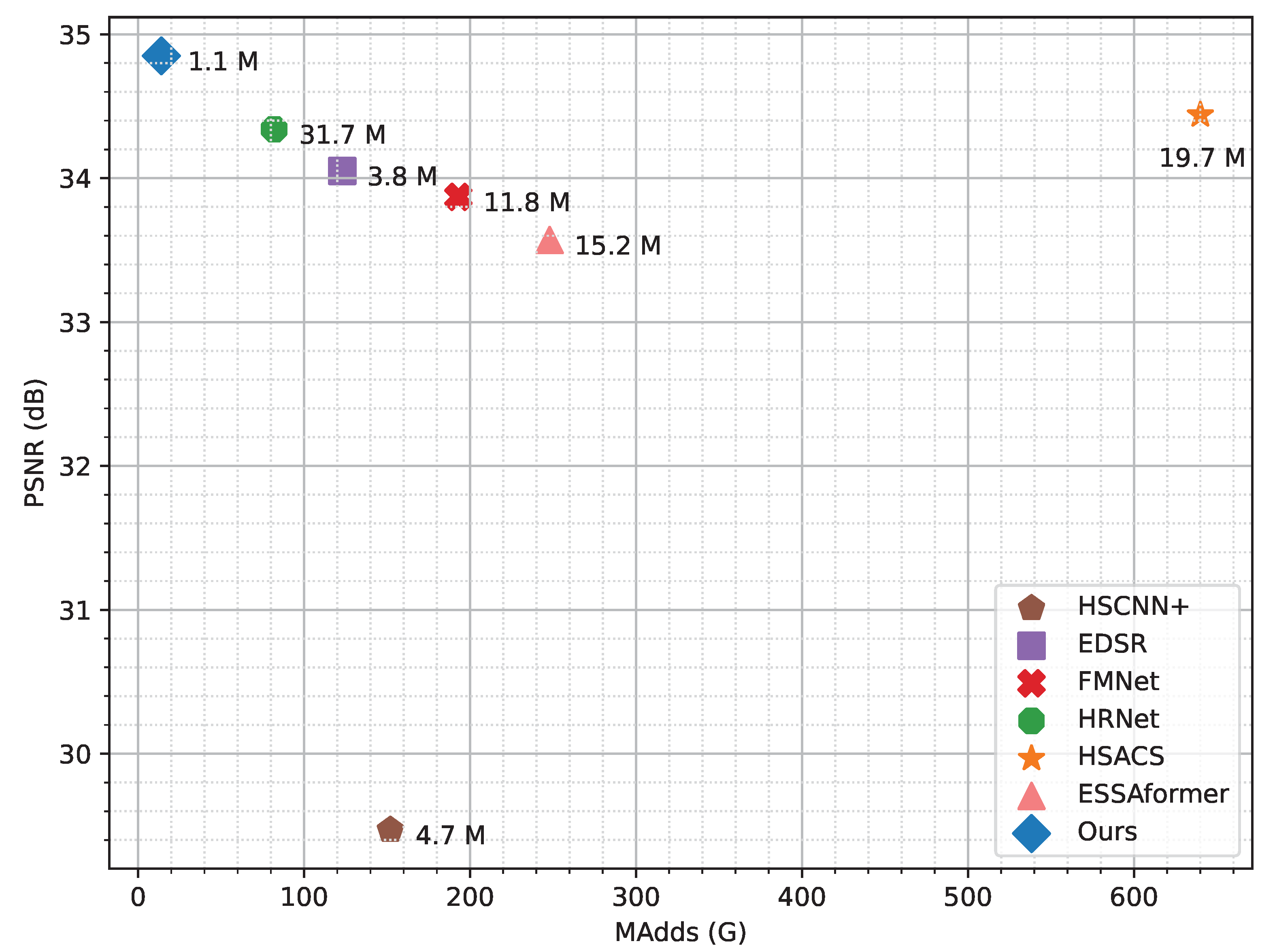
Accordingly, we propose a lightweight HSI reconstruction network, namely, Transformer with Convolutional Spectral Self-Attention (TCSSA). The network comprises both a CNN-Transformer encoder and a CNN-Transformer decoder, with CSSA blocks serving as the fundamental module. Unlike conventional U-shaped networks, TCSSA first uses a convolution to sample feature maps of RGB images in the spectral dimension into the CSSAB to obtain multiscale encoding and decoding features for HSIs. Meanwhile, resampling the spectral dimensions can effectively reduce the computational complexity. Then, the obtained encoded and decoded features are concatenated to leverage the comprehensive information spanning both spatial and spectral domains. As is well known, the spectra of HSIs are highly correlated between consecutive bands; meanwhile, the spatial information is strongly correlated with neighboring regions and weakly correlated with more distant regions. To extract spatial texture and global spectral correlations of HSIs more efficiently, we combine convolutions and self-attention in the transformer to design the CSSA, which is the basic unit of the CSSABs. Convolutions are used to extract spatially local features. Afterwards, self-attention is calculated across both spatial and spectral dimensions to effectively capture the spatial details and spectral characteristics of HSIs. As illustrated in Figure 1, the proposed TCSSA achieves a trade-off between reconstruction accuracy, multiply–add operations (MAdds), and parameters.
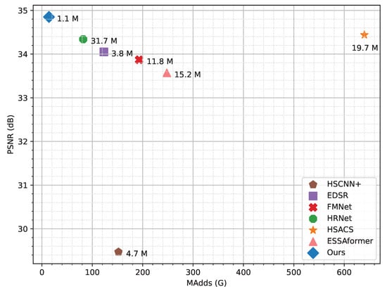
Figure 1.
Comparison of our proposed TCSSA model with other SSR models using the CAVE dataset. The horizontal axis represents multiply–add operations (MAdds), while the vertical axis depicts peak signal-to-noise ratio (PSNR). The points in the figure are labeled as the number of parameters. Our TCSSA approach exhibits a better tradeoff between its computational complexity (numbers of parameters and MAdds) and PSNR.
- (1)
- We propose an SSR network based on a combination of transformers and CNN. The network consists of multiple cascaded encoders and decoders that can efficiently extract spatial texture and spectral contextual features from HSIs.
- (2)
- The proposed CSSA, which combines a CNN and a self-attention mechanism, can compute spatial local self-attention and global spectral self-attention.
- (3)
- The proposed network effectively balances computational complexity with the quality of reconstruction achieved. The superiority of our approach is demonstrated on one remote sensing image dataset and two natural image datasets.
The rest of the paper is structured as follows. Section 2 provides an overview of related work, encompassing CNN-based SSR methods and transformer-based models. Section 3 elaborates on the proposed approach. Section 4 evaluates the effectiveness of our approach on three datasets. Section 5 provides a detailed discussion of our proposed method. Lastly, Section 6 summarizes the findings and concludes the paper.
2. Related Works
2.1. CNN-Based SSR Approaches
With the remarkable achievements demonstrated by CNNs in computer vision [22,23,24] and the continuous expansion of HSI datasets, researchers are increasingly turning to CNNs for SSR. Galliani et al. [25] enhanced a residual network derived from the U-Net architecture, employing it for spectral reconstruction tasks. This marked the first application of a deep learning approach to reconstructing HSIs from RGB images, and the authors achieved unprecedented performance. Their approach is an important node in the development of SSR. Xiong et al. [26] introduced HSCNN for recovering hyperspectral information from RGB and spectrally undersampled projections. Subsequently, the authors enhanced HSCNN by eliminating the upsampling operation and changing the residual blocks with dense blocks, obtaining an improved model named HSCNN+ [27]. Fu et al. [28] investigated the influence of camera spectral response (CSR) on hyperspectral image restoration and introduced a CSR selection layer to identify the most suitable CSR for each hyperspectral image. Inspired by residual dense networks [29], Zhao et al. [30] designed a multilevel high-resolution network (HRNet) comprised of residual dense blocks and residual global blocks to remove image residuals and enhance the perceptual domain, respectively. To better enhance the spatial resolution of HSIs while preserving their spectral characteristics, a hybrid convolution and spectral symmetry preservation network was proposed in [31]. Zhang et al. [32] designed a pixel-aware network with different receptive field sizes for SSR. However, the majority of approaches only emphasize local spatial information, often overlooking the modeling of spectral information [33,34].
With the development of attention mechanisms [35], many researchers have combined attention and CNN for SSR tasks. The primary function of an attention mechanism is to evaluate different dimensions of the input and assign weights to features based on their importance, thereby emphasizing the influence of significant features on downstream models [36]. The hybrid 2D–3D deep residual attentional network described in [33] has the ability to dynamically adjust channel and bandwidth feature responses to enhance contextual features; this was the first time that an attention mechanism was used for SSR. Adaptive weighted attention networks [37] reassign feature weights to channel dimensions by integrating correlations between channels. Li et al. [38] introduced a CNN-based method combining dual second-order attention and convolutional spectral self-attention to effectively analyze spatial–spectral information. He et al. [39] introduced a channel attention module that used trainable parameters to learn the spectral differences in different bands. Zhang et al. [40] designed a channel attention reconstruction network using a CNN that efficiently learns the spatial and spectral correlation in HSIs. Although the above techniques incorporate spectral information into their models, they still have a high level of parameterization and computational complexity.
2.2. Transformer-Based Models
Vision Transformer (ViT) [41] marked a breakthrough in computer vision tasks by employing the transformer architecture to process images as sequences, achieving outstanding performance. It has good scalability and has become a milestone in utilizing transformers for computer vision applications. Following ViT, researchers have developed a range of improved methods. To address the deficiency of local information in ViT, Swin Transformer [42] incorporates a shifted windows operation akin to CNN, enabling self-attention to be computed within each local window to extract image’s local features and mitigate computational complexity. Yuan et al. [43] proposed a Tokens-to-Token module (T2T) that combines neighboring tokens into a single token. T2T is performed iteratively to continuously aggregate neighboring tokens. Transformer-in-Transformer (TNT) [44] is designed with two transformer blocks; the outer transformer block captures the global relationship between the patch embedding, while the inner transformer block focuses on extracting local structure information from the pixel embedding. To reduce the training time, Data-efficient image Transformers (DeiT) [45] introduced a strategy of knowledge distillation in transformers.
In the hyperspectral direction, Cai et al. [18] proposed a transformer-based method for HSI reconstruction called Coarse-to-fine Sparse Transformer (CST), embedding the sparsity of HSIs into deep learning-based algorithms. CST first employs a spectra-aware screening mechanism (SASM) for coarse patch selection; subsequently, the selected patches are fed into spectra-aggregation hashing multi-head self-attention (SAH-MSA) for fine-grained pixel clustering and self-similarity capture. To address the issue of underutilized spectral information and artifacts in the upsampled data, Zhang et al. [19] proposed an efficient transformer for hyperspectral image superresolution, referred to as ESSAformer. They introduced a robust and spectral-friendly similarity metric called the Spectral Correlation Coefficient (SCC) and proposed an efficient SCC-kernel-based self-attention (ESSA), which reduces attention computation to linear complexity. ESSA enlarges the receptive field of upsampled features without extensive computation, enabling the model to effectively utilize spatial–spectral information at different scales, thereby producing more natural high-resolution images.
2.3. Architectures Combining CNN and Transformer
In an effort to merge the strengths of CNN and transformer architectures, co-scale Conv-attentional image Transformers (CoaT) [46] were proposed as a conv-attention module to exploit convolutions in positional encoding and the relative position embedding within the factorized attention module to improve computational efficiency. Convolutional ViT (ConViT) [47] investigated the importance of inductive bias in transformers and explored integrating a CNN and transformer. Aiming to address interpretability issues, the unmixing-guided convolutional transformer network was introduced in [48], integrating transformer and resBlock components within a paralleled framework. Convolution vision Transformer (CvT) [49] utilizes CNN before computing self-attention, which can provide the model with the advantages of CNNs in terms of translation, scaling, and deformation invariance. LocalViT [50] and Pyramid Vision Transformer (PVT v2) [51] add depthwise convolution to extract local information by using a CNN after computing self-attention. Lite Vision Transformer (LVT) [52] combines both self-attention and convolutions by exploiting local self-attention in a kernel of size . Restoration Transformer (Restormer) [53] uses CNN to aggregate local information before calculating self-attention and obtains the global spectral features by computing cross-channel covariance matrices in the spectral dimension. EdgeNeXt [54] uses depthwise convolution and cross-channel self-attention to capture multiscale spatial and spectral features from images.
The above methods are not applicable to SSR tasks. Extracting the spatial texture features via CNN lacks the ability to capture the local spatial self-similarity. Unlike the above methods, TCSSA first utilizes grouped convolution as the linear mapping operation and extracts the local spatial features. Afterwards, local spatial and global spectral self-attention are computed in the spatial–spectral dimension to effectively grasp the local spatial similarity and global spectral similarity of the HSIs.
3. Proposed Method
3.1. Architecture of TCSSA
Let denote an RGB image and let denote the corresponding HSI reconstructed from . Here, C represents the number of channels in the HSI while W and H denote its width and height, respectively. Reconstructing HSIs from RGB images poses a significantly ill-posed challenge, particularly when C assumes large values. The SSR problem can be expressed as follows:
where represents the transition matrix from to , while and are the matrices unfolded from and .
The proposed TCSSA is mainly composed of a CNN-Transformer encoder and a CNN-Transformer decoder, as illustrated in Figure 2, TCSSA operates with as its input; after the action of multiple cascaded encoders and decoders, it then outputs with rich spectral information.

Figure 2.
The structure of the proposed TCSSA, primarily comprising a CNN-Transformer encoder and a CNN-Transformer decoder.
3.1.1. CNN-Transformer Encoder
The initial step involves passing the provided RGB image through a convolutional layer to capture low-level features. The obtained feature map adds a skip connection before entering the encoding module to ensure the preservation of the foundational characteristics inherent in the RGB image. The encoding module E, comprising a convolutional layer and a CSSAB, is capable of extracting profound spatial and spectral contextual features. The output from the k-th encoding module can is formulated as
where n represents the total count of encoding modules. When , represents the input of the first encoding module; when k∈ {2,⋯, n}, and represent the input and output of the k-th encoding module, where and denote the number of channels of and , respectively. After each encoding module, a skip connection is introduced to preserve deep spatial and spectral information by linking the output of the k-th encoding module with the input of the -th decoding module.
3.1.2. CNN-Transformer Decoder
After the output of the CNN-Transformer encoder, we incorporate a convolutional layer as an intermediate transition layer to perform feature mapping before proceeding to the CNN-Transformer decoder. Then, the deep spatial and spectral information extracted by the CNN-Transformer encoder is decoded by n decoding modules. Each decoding module D includes a spectral downsampling layer, a CSSAB, and a convolution. The expression for the output from the k-th decoding module is as follows:
When , represents the input of the first decoding module. When k, and are concatenated (Cat) to obtain the input of the k-th decoding module, outputting , which is in the dimension of . is concatenated with to generate an augmented feature representation. In the end, undergoes a convolutional operation to produce the decoded feature map. The recovered HSI is obtained by summing the feature map and .
3.2. CSSAB
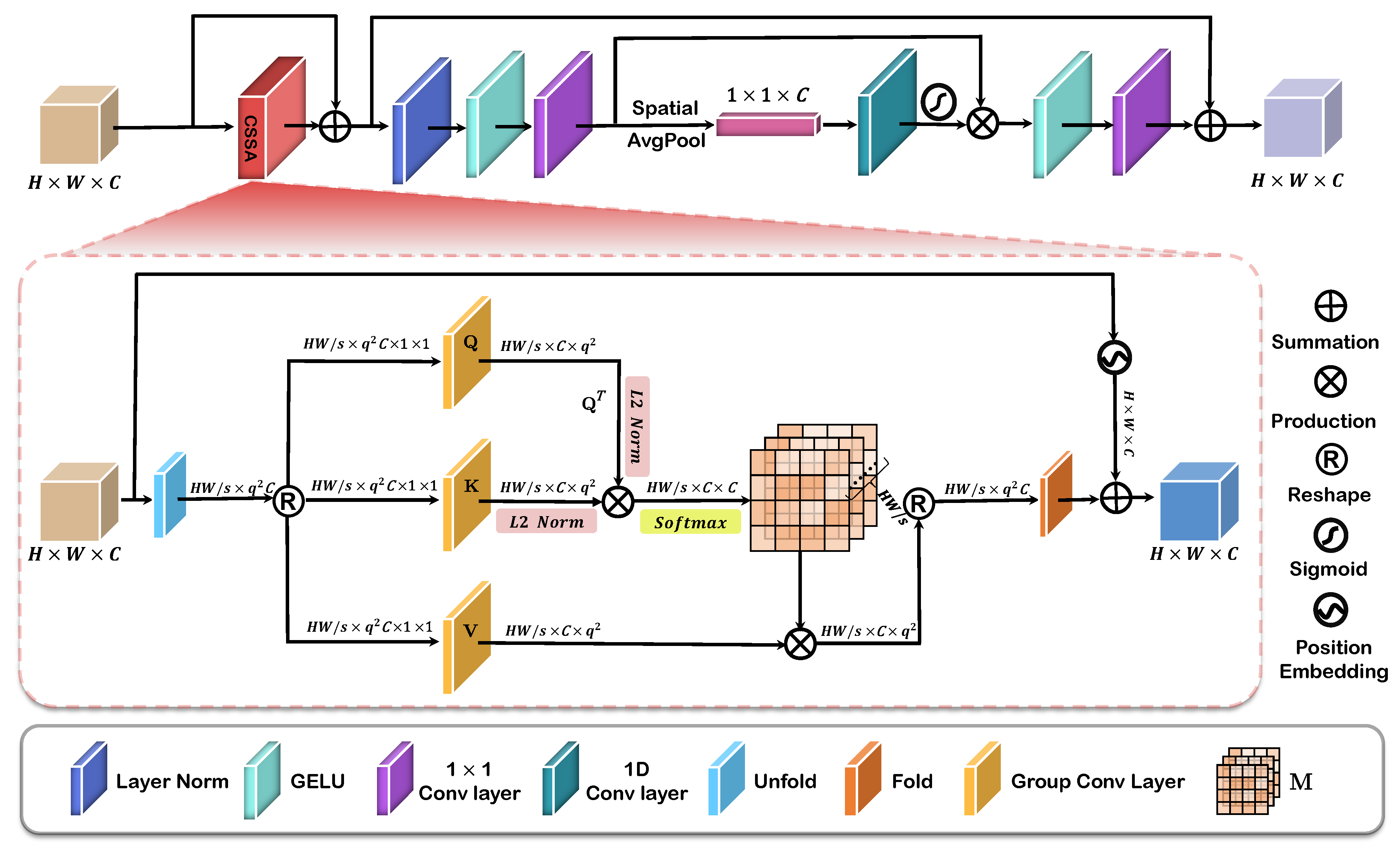
The convolutional spectral self-attention block (CSSAB) is depicted in Figure 3. First, skip connections are introduced to alleviate information loss, followed by the extraction of vital features from the spatial and spectral dimensions of HSI using CSSA. The resulting output passes through a normalization layer, a Gaussian Error Linear Unit (GELU) activation function, and convolution to obtain the feature maps. Efficient channel attention (ECA) [55] is employed for learning the weights of each channel. Initially, ECA conducts spatially averaged pooling on the input, yielding a vector with dimensions of . Subsequently, it employs one-dimensional convolution to acquire the channel weight coefficients. The obtained weight vector is passed through a sigmoid activation function, and the resulting output is utilized to modify the channel weights by element-wise multiplication with the skip connection output. After passing through a GELU activation function and a convolution, the feature map corresponding to the adjusted channel weights is combined with the skip connection output, resulting in the generation of the final high-dimensional feature map.

Figure 3.
Illustrations of CSSAB and CSSA.
3.3. CSSA
Convolutional operations are particularly effective in capturing the spatial contextual intricacies of images [56]. Therefore, this paper proposes a CSSA mechanism, as shown in Figure 3. Given a normalized tensor , the dimension of is extended to by the function [57], where q and s represent the scale of the sliding window and stride in the function, respectively. The function is utilized for extracting sliding local blocks from a batch of input tensors, resulting in a two-dimensional output tensor. We use to denote the tensor after the reshaping operation. Then, group convolutions are applied to compute the projections of the query (), key (), and value (). The input tokens = , = and = of the attention function can be generalized as
where Conv represents the grouped convolution operation. Subsequently, , , and are segmented into N heads, with each segment organized along the spectral dimension. Next, the L2 norm of and is calculated to make the model more stable during training. We perform a dot product operation across the spatial–spectral dimension between and to produce an attention matrix of dimension . Subsequently, this matrix is fed into the function to obtain the softmax-scaled attention score matrix . The following represents the attention mechanism, labeled as :
where is the learnable weight coefficient. After the and functions, the dimensions of are and . The function is the inverse of the function. Finally, the output is obtained by adding the position embedding that is learned by the convolutional network.
4. Experiments
4.1. Datasets and Evaluation Metrics
4.1.1. Remote Sensing Image Dataset
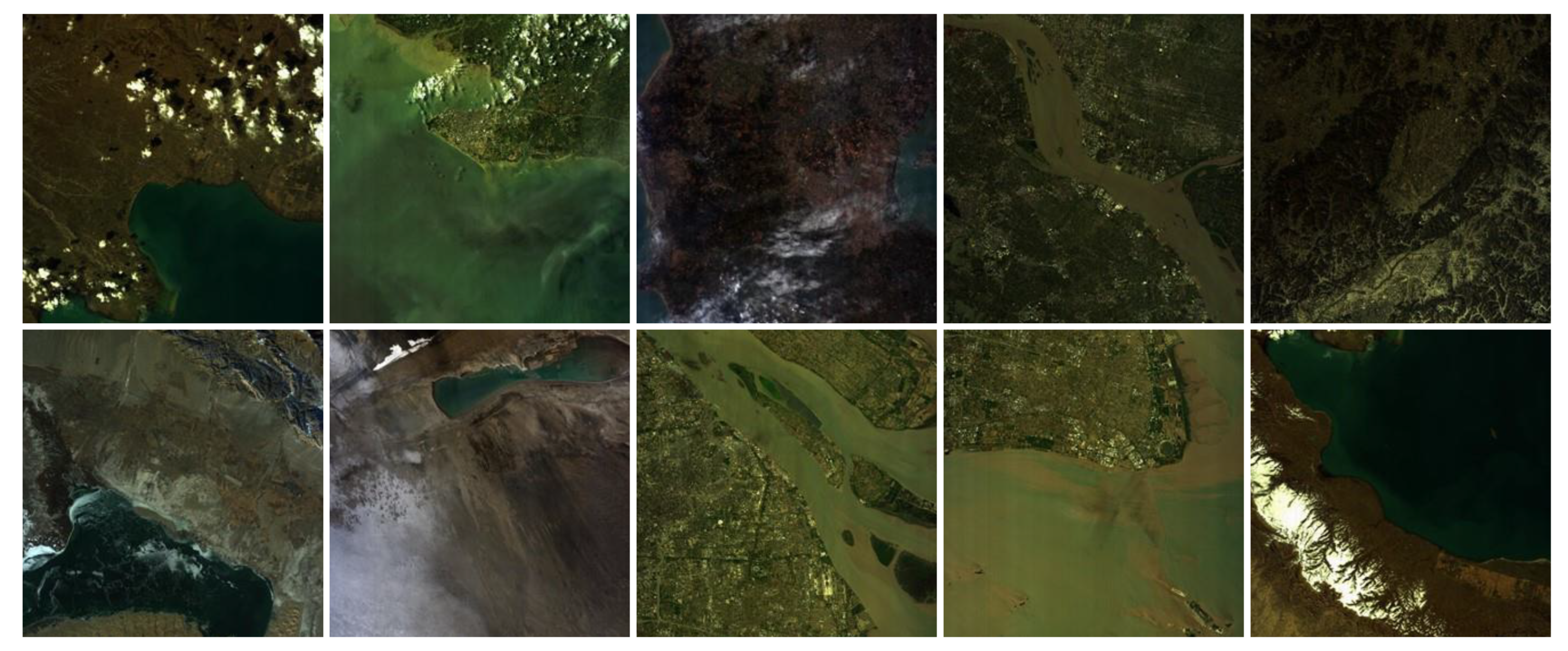
We created a remote sensing image dataset named GF5, which contains Chinese Gaofen-5 satellite images. The dataset is accessible at http://jiasen.tech/ on 1 June 2024. HSIs in GF5 have a variety of scenes, such as urban, mountain, farmland, river, lake, harbors, etc. Figure 4 shows ten examples of different scenarios from the GF5 dataset. The original HSIs were calibrated to digital numbers (DNs) in the range of 0–65,535 with a spectral range of 390–1035 nm in 150 bands at a spectral resolution of 5 nm. The RGB images were thumbnail images in Gaofen-5 production. All images in GF5 were normalized to [0, 1] using the min–max normalization method. The spatial size of HSIs and RGBs were readjusted to , resulting in a total of 1715 image pairs, with 1500 pairs randomly chosen as the training data, 50 pairs as the validation data, and 50 pairs as the test data.

Figure 4.
Ten example scenes of remote sensing images in the GF5 dataset displayed in RGB.
4.1.2. Natural Image Datasets
We also select two public natural image datasets CAVE [58] and NTIRE2022 [59], to assess the efficacy of the proposed TCSSA.
CAVE contains 32 sets of paired RGB-HSI images, with each HSI featuring spatial dimensions of and 31 consecutive spectral bands ranging from 400 nm to 700 nm at intervals of 10 nm. We standardized all images in CAVE to fall within the range of [0, 1] using the min–max normalization technique. Next, one image from each scene was chosen as the test dataset, while the remaining images were designated as the training dataset.
NTIRE2022 is the dataset that was used for the 2022 Spectral Reconstruction Competition. The scenes in this dataset are very diverse. The dataset comprises 1000 paired images, with 900 designated for training, 50 for validation, and another 50 for testing purposes. As the test data are not public available, we utilized the validation images for evaluating our model. The original HSIs consist of 204 spectral bands spanning wavelengths from 400 to 1000 nm. Each image was resampled to 31 spectral bands with wavelengths from 400 nm to 700 nm, with a 10 nm interval between each band. The spatial dimensions of each image are .
4.1.3. Evaluation Metrics for SSR
In this paper, we chose various evaluation metrics on different datasets to assess the proposed method. The performance of TCSSA on the NTIRE2022 dataset was quantitatively evaluated using the root mean square error (RMSE), mean relative absolute error (MRAE), peak signal-to-noise ratio (PSNR), and structural similarity index measure (SSIM) [60]. The evaluation metrics used on the CAVE and GF5 datasets were RMSE, PSNR, spectral angle mapping (SAM) [61], and SSIM.
Greater PSNR and SSIM values correlate with reduced MRAE, SAM, and RMSE, suggesting superior performance. The formulas for MRAE and RMSE are as follows:
where and represent the value of the j-th pixel value in band i of the ground truth and the reconstructed HSI, respectively, M is the total number of bands, and N is the total number of pixels in the image. In the formula for calculating SSIM, , , , and represent the mean and standard deviation of the ground truth image and the reconstructed HSI, while represents the covariance between the ground truth image and the reconstructed HS and and are small constants used for numerical stability.
4.2. Implementation Settings
The paired RGB images and HSIs in GF5, CAVE, and NTIRE2022 were all cropped to for training. The training batch size was 20 and n was set to 3. As proposed, the TCSSA model undergoes optimization utilizing the Adam optimizer with specific parameters: , and . The initial learning rate was established at 0.0004, with training concluding after 250 epochs on GF5 and NTIRE2022 datasets and 100 epochs on CAVE. The PyTorch framework was utilized for all experiments, leveraging the computational power of an NVIDIA A40 GPU and an Intel(R) Xeon(R) Silver 4314 CPU. The optimization strategy in this research revolves around employing MRAE as the loss function, which provides a quantitative assessment of the disparity between the ground truth and the reconstructed HSI.
4.3. Comparisons With State-of-the-Art Methods
The effectiveness of the proposed TCSSA model was evaluated against six state-of-the-art methods: HSCNN+ [27], FMNet [32], HRNet [30], EDSR [62], HSACS [38], and ESSAformer [19] across the GF5, CAVE, and NTIRE2022 datasets. HSCNN+, FMNet, and HRNet represent three established deep learning-based SSR methods in the comparison, while EDSR is a spatial superresolution model and HSACS is a state-of-the-art SSR method based on a deep hybrid 2D–3D CNN.
4.3.1. Quantitative and Visual Results Obtained on GF5
The GF5 dataset contains remote sensing images that have complex spatial information and 150 spectral bands, which makes them more difficult to restore from RGB images. The proposed method, along with other state-of-the-art approaches, was applied to the validation and test datasets from GF5. The quantitative results are showcased in Table 1. The results obtained from the validation data indicate that TCSSA surpasses the other SSR methods across all four evaluation criteria. On the test data, HRNet slightly outperforms TCSSA in terms of the SSIM metric, while TCSSA outperforms the other SSR methods in RMSE, PSNR, and SAM metrics.

Table 1.
Quantitative results of different methods on both validation and test data in GF5. The optimal outcomes are emphasized in bold.
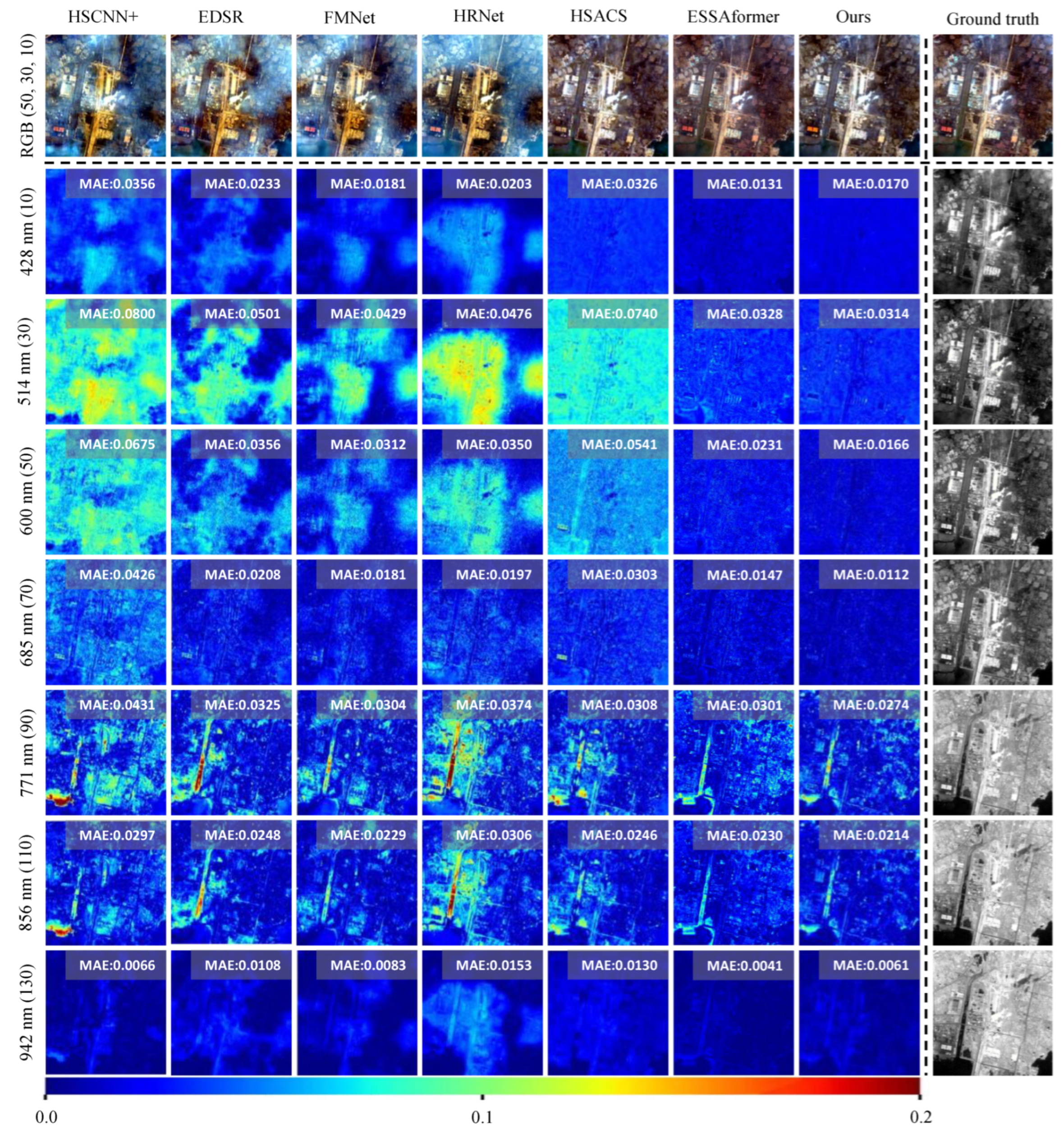
To analyze the reconstruction results across various bands, we compared the absolute error maps of seven distinct bands from a sample image in the GF5 test dataset, as depicted in Figure 5. The wavelengths of seven bands are 428 nm (band 10), 514 nm (band 30), 600 nm (band 50), 685 nm (band 70), 771 nm (band 90), 856 nm (band 110), and 942 nm (band 130). The image contains a variety of features, such as buildings, rivers, farmlands, and oceans, which bring a great challenge to the SSR task. For band 10 reconstructed by HSACS and our method, there is nearly no difference between the recovered band and ground truth. The model’s reconstruction performance notably surpasses that of HSACS and FMNET and other algorithms, particularly on bands 30, 50, and 70. Due to the longer wavelengths of band 90 and band 110, the reflectance of different objects varies greatly, which makes spectral reconstruction difficult. It is noteworthy that there is a significant disparity in the reconstruction results of the river, building, and estuary areas across different methods. The performance of TCSSA in these regions is still superior to that of the other SSR methods. Two images with different scenes were selected from the validation dataset of GF5 to evaluate the performance of the proposed TCSSA on real-world data, with the results shown in Figure 6. Four locations with different land covers are labeled in blue, red, yellow, and green colors on the images. We plotted the real spectral curves of the four locations and the spectral response curves reconstructed by TCSSA. As seen from the figure, the spectral fidelity of the four reconstructed ground features is excellent, indicating the superior spectral reconstruction capability of our method.
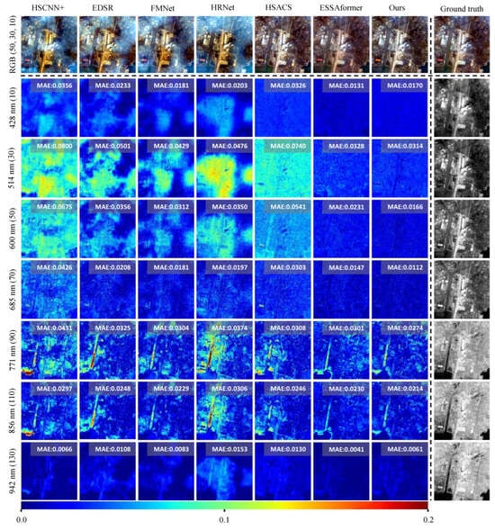
Figure 5.
Qualitative results of an example image from the test data in GF5. The top row displays the restored true-color RGB composites of bands 50 (600 nm), 30 (514 nm), and 10 (428 nm) by all methods and ground truth. The second to eighth rows are the results of absolute error maps corresponding to seven reconstructed spectral bands at different wavelengths and ground truth. The MAE value on the top right corner of each absolute error map represents the mean absolute error of that map.
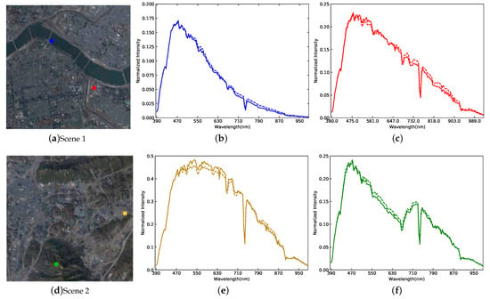
Figure 6.
(a,d) are two scenes from the validation data in GF5, while (b,c) are the spectral curves of the blue and red points in (a) and (e,f) are the spectral curves of the yellow and green points in (d). The solid and dashed lines represent the ground truth and the spectral signature recovered by the proposed method.
4.3.2. Quantitative and Visual Results Obtained on CAVE and NTIRE2022
Table 2 presents the quantitative evaluation results obtained on the natural image datasets. On the CAVE dataset, TCSSA achieves a reduction of 0.23 in RMSE and 0.48 in SAM while increasing SSIM by 0.0047 and PSNR by 0.41 dB compared with the HSACS method. Compared with the classic HSCNN+ and HRNet approaches on the NTIRE2022 dataset, TCSSA reduces the MRAE by 0.2043 and 0.1761 and improves PSNR by 7.13 dB and 6.14 dB. Our approach achieves superior performance compared to the other six methods on the test data in CAVE and the validation data in NTIRE2022.

Table 2.
Quantitative results of different methods on the test data in CAVE and validation data in NTIRE2022. The optimal outcomes are emphasized in bold.
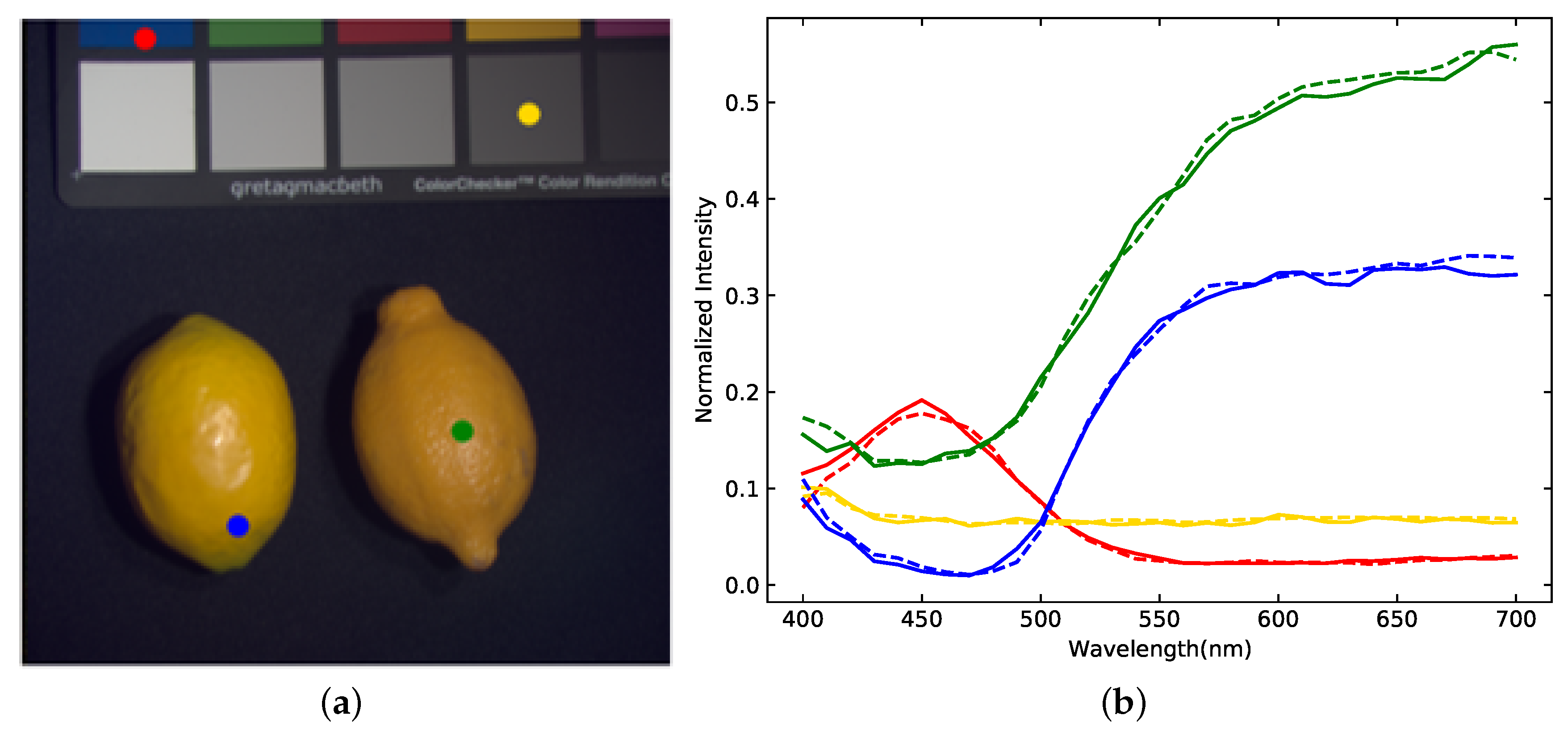
To assess the perceptual quality of the proposed TCSSA, we present the mean absolute error map between the reconstructed image (Fake and Real Lemons) and the ground truth in CAVE in Figure 7. The error map of HSCNN+ has the most errors, which are concentrated around the fake lemon (left). The band recovered by our method closely resembles the ground truth and outperforms the other methods. Additionally, we selected four points within the lemons, and their spectral curves, reconstructed by our method, are illustrated in Figure 8. It is evident that the four spectral responses are all approximately the same as the responses of the ground truth. In summary, our method concurrently restores both the spatial and spectral detail of the image.

Figure 7.
Qualitative results of lemons in CAVE. The top row exhibits reconstructed images at band 31 obtained from different SSR methods, while the bottom row displays the corresponding mean absolute error maps.

Figure 8.
(a) RGB image of Fake and Real Lemons in CAVE with four selected points. (b) The spectral curves of four points obtained by our method and the ground truth are plotted by the dashed lines and solid lines, respectively.
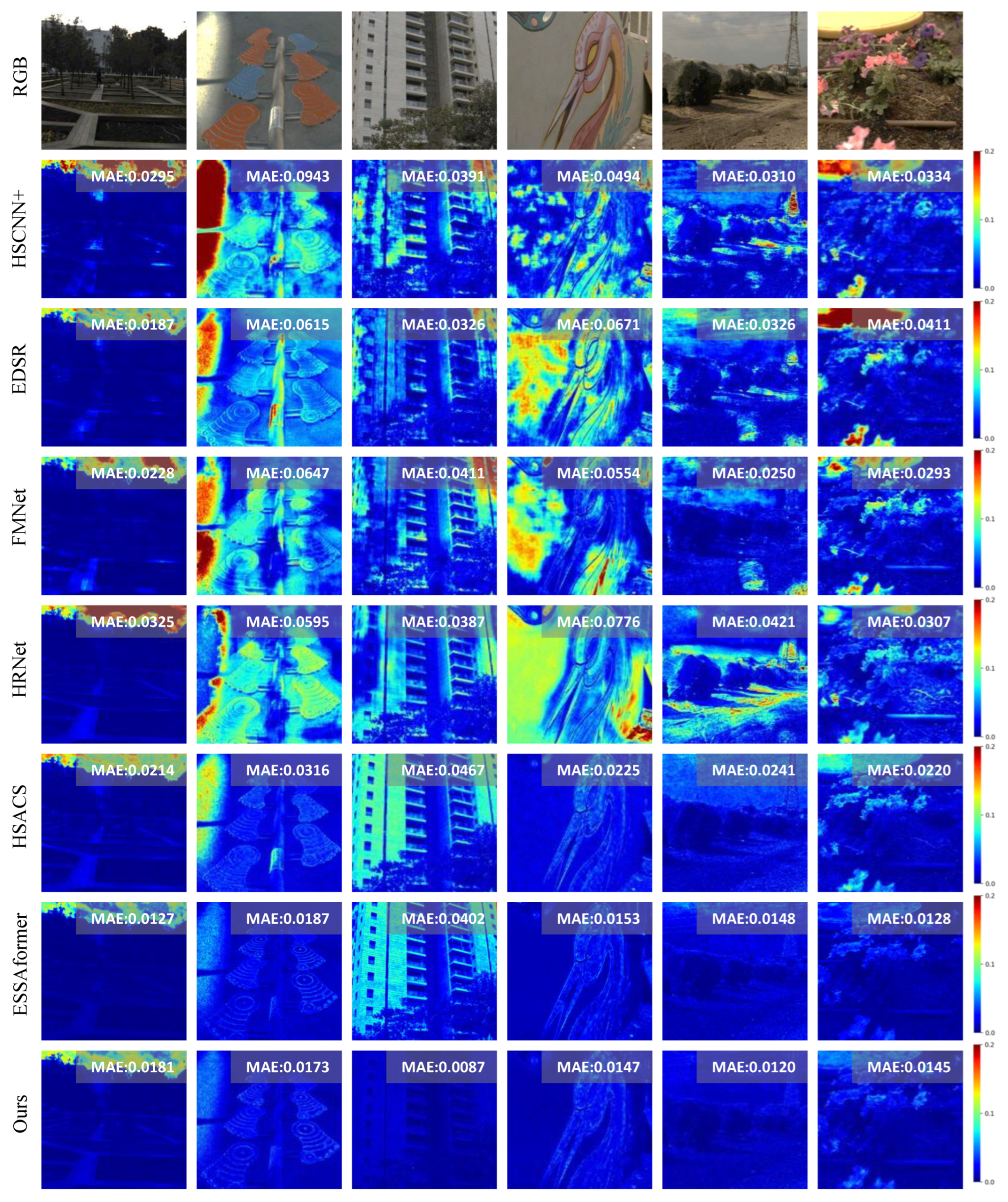
Figure 9 shows the qualitative results on the NTIRE2022 dataset. We selected six images from the validation data and compared the error maps of the SSR results. It can be seen that the competing methods retain considerable texture information. Our method has the minimum reconstruction error, which implies that the proposed TCSSA achieves good performance in recovering the hyperspectral bands.
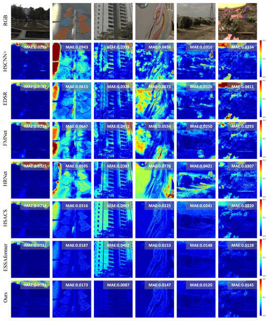
Figure 9.
Qualitative results of six example images from the validation data in NTIRE2022. The initial row displays the RGB images, while the subsequent rows (second to eighth) depict the absolute error maps corresponding to different SSR methods. The MAE value on the top right corner of each absolute error map represents the mean absolute error of that map.
To further compare the outcomes of various methods, we selected four RGB images from the NTIRE2022 dataset in which one random location in each of four images is labeled by a red dot, as shown in Figure 10. Displayed on the right, spectral response curves depict the comparison between the reconstructed results from all methods and the ground truth for these positions. It can be observed that the spectral curve reconstructed by TCSSA closely resembles the ground truth curve compared to other methods. This can be attributed to TCSSA’s capability to learn global spectral self-attention and retain intricate spectral details within the image.
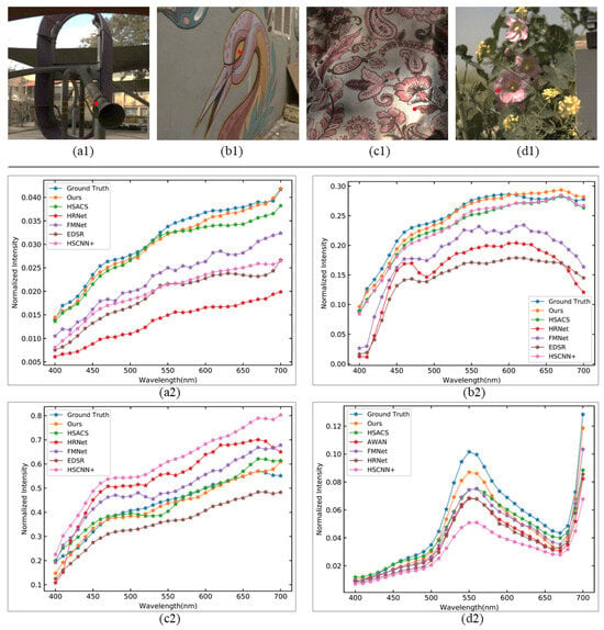
Figure 10.
(a1–d1) The top row displays four RGB images selected from NTIRE2022. (a2–d2) Below are the spectral curves corresponding to the marked red dot in the four RGB images obtained through different SSR methods.
Table 3 demonstrates the number of parameters (Params), the number of multiply-add operations (MAdds), the memory footprint (Memory), and the test time achieved by all SSR methods on the test data of CAVE. Params, MAdds, and Memory can reveal the computational complexity of different methods. MAdds and Memory were measured on an image patch with a size of . The test time of each method was calculated on six reconstructed HSIs. TCSSA only needs 1.08 M parameters and 14 G MAdds, which requires the lowest computational cost among all approaches. Specifically, params compared to HSACS, FMNet, and HSCNN+ are reduced by 94.53%, 90.82%, and 76.77%, respectively. Regarding the test time, TCSSA runs approximately eight times faster than HSACS, which is the second best SSR method, and has almost the same time as EDSR, whereas its reconstruction performance is far from ours. Overall, our proposed method achieves a tradeoff between reconstructed image fidelity, computational complexity, and time efficiency.

Table 3.
Comparison of computational complexity and test time of different SSR methods. MAdds and Memory were measured on an image patch with size . The test time was calculated on six reconstructed HSIs in CAVE.
4.4. Ablation Analysis
To validate the effectiveness of CSSA and to explore the influence of the number n of encoding modules E in the CNN-Transformer encoder and number of decoding modules D in the CNN-Transformer decoder, we conducted ablation experiments using the validation data from NTIRE2022.
4.4.1. Effectiveness of the CSSA
To evaluate the effectiveness of CSSA, which integrates CNN with the self-attention mechanism in transformer, we conducted ablation experiments comparing two alternative self-attention mechanisms: convolutional self-attention (CSA) [52] and multi-Dconv head transposed attention (MDTA) [53]. The results are recorded in Table 4. The backbone was obtained by eliminating CSSA from TCSSA. , , and denote the models with CSA, MDTA, and, CSSA, respectively. The performance of , , and exhibits an improvement in MRAE by 0.0643, 0.0914, and 0.0938, respectively, compared with the baseline . Moreover, achieves superior RMSE and PSNR values, underscoring the superiority of CSSA over CSA and MDTA.

Table 4.
Evaluation of our method’s performance with various self-attention modules on the validation data from NTIRE2022.
4.4.2. Effect of Number N
To analyze the influence of the number of encoding and decoding modules on the TCSSA performance, we used different n values to conduct the experiments. The results are recorded in Table 5. Obviously, when , as the model’s parameter count and MAdds rise, notable enhancements in performance metrics such as MRAE, RMSE, and PSNR are evident. When , the model’s parameter count and MAdds increase approximately four times compared with the number when , while the MRAE increases by 0.0268, the RMSE increases by 0.0049, and the PSNR decreases by 0.98 dB. Therefore, we chose in the experiments to balance computational complexity and spectral reconstruction performance.

Table 5.
Evaluation of our method’s performance with different values of n on the validation data from NTIRE2022.
5. Discussion
TCSSA effectively captures both the local spatial similarity and global spectral similarity of HSIs, leading to promising outcomes in spectral superresolution. However, there are some limitations present in TCSSA. First, as the proposed method focuses on the reconstruction of spectral channels, the CSSA attention mechanism designed in this study exhibits less capability in extracting spatial information than spectral information. Second, in practical applications RGB images often contain some level of noise or contamination. Our approach does not address this issue. When significant noise or contamination is present in RGB images, additional processing steps for noise or contamination removal are necessary to achieve more robust reconstruction results.
6. Conclusions
This paper presents a Transformer-based network with Convolutional Spectral Self-Attention (TCSSA) for the reconstruction of HSIs from RGB images. The spatial and spectral information can be efficiently restored through multiple cascaded encoding and decoding modules. By resampling HSIs in the spectral dimension, TCSSA effectively reduces the computational cost associated with self-attention calculations within the model. To establish the mappings between RGB images and HSIs more efficiently, we design a CSSA mechanism by combining a CNN with self-attention to calculate the spatial local self-attention and global spectral self-attention. Experimental results on one remote sensing image dataset and two natural image datasets highlight the superiority and effectiveness of the proposed approach compared to six state-of-the-art SSR methods. Furthermore, TCSSA stands out for its efficiency, demanding fewer parameters, MAdds, and testing time all while maintaining an optimal equilibrium between computational complexity and SSR efficacy.
Author Contributions
Conceptualization, M.X. and X.L.; methodology, M.X. and X.L.; software, L.H. and J.M.; validation, L.H. and J.M.; formal analysis, L.H., J.M. and M.X.; investigation, L.H. and J.M.; resources, J.M. and M.X.; data curation, L.H. and J.M.; writing—original draft preparation, X.L. and M.X.; writing—review and editing, X.L., L.H., J.M. and M.X.; visualization, L.H. and M.X.; supervision, M.X.; project administration, M.X.; funding acquisition, M.X. All authors have read and agreed to the published version of the manuscript.
Funding
This work was supported by the National Natural Science Foundation of China under Grant 42271336, Guangdong Basic and Applied Basic Research Foundation (Grant No. 2024A1515011079), Shenzhen Special Sustainable Development Science and Technology Project (Grant No. KCXFZ20211020164015024), and the Research Team Cultivation Program of Shenzhen University (Grant No. 2023JCT002).
Data Availability Statement
The source code and data of this article will be made publicly available at http://jiasen.tech/ for reproducible research.
Conflicts of Interest
The authors declare no conflicts of interest.
References
- Fauvel, M.; Tarabalka, Y.; Benediktsson, J.A.; Chanussot, J.; Tilton, J.C. Advances in Spectral-Spatial Classification of Hyperspectral Images. Proc. IEEE 2012, 101, 652–675. [Google Scholar] [CrossRef]
- Manolakis, D.; Shaw, G. Detection Algorithms For Hyperspectral Imaging Applications. IEEE Signal Process. Mag. 2002, 19, 29–43. [Google Scholar] [CrossRef]
- Li, J.; Bioucas-Dias, J.M.; Plaza, A. Spectral–Spatial Hyperspectral Image Segmentation Using Subspace Multinomial Logistic Regression and Markov Random Fields. IEEE Trans. Geosci. Remote Sens. 2011, 50, 809–823. [Google Scholar] [CrossRef]
- Ma, Q.; Jiang, J.; Liu, X.; Ma, J. Multi-Task Interaction Learning for Spatiospectral Image Super-Resolution. IEEE Trans. Image Process. 2022, 31, 2950–2961. [Google Scholar] [CrossRef] [PubMed]
- Kaya, B.; Can, Y.B.; Timofte, R. Towards Spectral Estimation from a Single RGB Image in the Wild. In Proceedings of the 2019 IEEE/CVF International Conference on Computer Vision Workshop (ICCVW), Seoul, Republic of Korea, 27–28 October 2019; pp. 3546–3555. [Google Scholar]
- Zhu, Z.; Liu, H.; Hou, J.; Jia, S.; Zhang, Q. Deep Amended Gradient Descent for Efficient Spectral Reconstruction from Single RGB Images. IEEE Trans. Comput. Imaging 2021, 7, 1176–1188. [Google Scholar] [CrossRef]
- Arad, B.; Ben-Shahar, O. Sparse Recovery of Hyperspectral Signal from Natural RGB Images. In Proceedings of the European Conference on Computer Vision, Amsterdam, The Netherlands, 11–14 October 2016; Springer: Berlin/Heidelberg, Germany, 2016; pp. 19–34. [Google Scholar]
- Heikkinen, V. Spectral Reflectance Estimation Using Gaussian Processes and Combination Kernels. IEEE Trans. Image Process. 2018, 27, 3358–3373. [Google Scholar] [CrossRef] [PubMed]
- Gao, L.; Hong, D.; Yao, J.; Zhang, B.; Gamba, P.; Chanussot, J. Spectral Superresolution of Multispectral Imagery with Joint Sparse and Low-Rank Learning. IEEE Trans. Geosci. Remote Sens. 2020, 59, 2269–2280. [Google Scholar] [CrossRef]
- Akhtar, N.; Mian, A. Hyperspectral Recovery from RGB Images using Gaussian Processes. IEEE Trans. Pattern Anal. Mach. Intell. 2020, 42, 100–113. [Google Scholar] [CrossRef] [PubMed]
- Jia, Y.; Zheng, Y.; Gu, L.; Subpa-Asa, A.; Lam, A.; Sato, Y.; Sato, I. From RGB to Spectrum for Natural Scenes via Manifold-Based Mapping. In Proceedings of the IEEE International Conference on Computer Vision, Venice, Italy, 22–29 October 2017; pp. 4705–4713. [Google Scholar]
- Aeschbacher, J.; Wu, J.; Timofte, R. In Defense of Shallow Learned Spectral Reconstruction from RGB Images. In Proceedings of the IEEE International Conference on Computer Vision Workshops, Venice, Italy, 22–29 October 2017; pp. 471–479. [Google Scholar]
- Timofte, R.; De Smet, V.; Van Gool, L. A+: Adjusted Anchored Neighborhood Regression for Fast Super-Resolution. In Proceedings of the Asian Conference on Computer Vision, Singapore, 1–5 November 2014; Springer: Berlin/Heidelberg, Germany, 2014; pp. 111–126. [Google Scholar]
- Yan, Y.; Zhang, L.; Li, J.; Wei, W.; Zhang, Y. Accurate spectral super-resolution from single RGB image using multi-scale CNN. In Proceedings of the Chinese Conference on Pattern Recognition and Computer Vision (PRCV), Guangzhou, China, 23–26 November 2018; Springer: Berlin/Heidelberg, Germany, 2018; pp. 206–217. [Google Scholar]
- Wu, C.; Li, J.; Song, R.; Li, Y. Spectral Super-Resolution Using Hybrid 2D-3D Structure Tensor Attention Networks with Camera Spectral Sensitivity Prior. In Proceedings of the IGARSS 2020–2020 IEEE International Geoscience and Remote Sensing Symposium, Waikoloa, HI, USA, 17 February 2021; pp. 1857–1860. [Google Scholar]
- Hang, R.; Li, Z.; Liu, Q.; Bhattacharyya, S.S. Prinet: A Prior Driven Spectral Super-Resolution Network. In Proceedings of the 2020 IEEE International Conference on Multimedia and Expo (ICME), London, UK, 6–10 July 2020; pp. 1–6. [Google Scholar]
- Vaswani, A.; Shazeer, N.; Parmar, N.; Uszkoreit, J.; Jones, L.; Gomez, A.N.; Kaiser, Ł.; Polosukhin, I. Attention Is All You Need. Adv. Neural Inf. Process. Syst. 2017, 30, 5998–6008. [Google Scholar]
- Cai, Y.; Lin, J.; Hu, X.; Wang, H.; Yuan, X.; Zhang, Y.; Timofte, R.; Van Gool, L. Coarse-to-Fine Sparse Transformer for Hyperspectral Image Reconstruction. In Proceedings of the Computer Vision—ECCV 2022, Tel Aviv, Israel, 23–27 October 2022; pp. 686–704. [Google Scholar]
- Zhang, M.; Zhang, C.; Zhang, Q.; Guo, J.; Gao, X.; Zhang, J. ESSAformer: Efficient Transformer for Hyperspectral Image Super-resolution. In Proceedings of the 2023 IEEE/CVF International Conference on Computer Vision (ICCV), Paris, France, 1–6 October 2023; pp. 23016–23027. [Google Scholar]
- Carion, N.; Massa, F.; Synnaeve, G.; Usunier, N.; Kirillov, A.; Zagoruyko, S. End-to-End Object Detection with Transformers. In Proceedings of the European Conference on Computer Vision, Glasgow, UK, 23–28 August 2020; Springer: Berlin/Heidelberg, Germany, 2020; pp. 213–229. [Google Scholar]
- Shen, Z.; Bello, I.; Vemulapalli, R.; Jia, X.; Chen, C.H. Global Self-Attention Networks for Image Recognition. arXiv 2020, arXiv:2010.03019. [Google Scholar]
- Zhang, K.; Zuo, W.; Gu, S.; Zhang, L. Learning Deep CNN Denoiser Prior for Image Restoration. In Proceedings of the IEEE Conference on Computer Vision and Pattern Recognition, Honolulu, HI, USA, 21–26 July 2017; pp. 3929–3938. [Google Scholar]
- Asgari Taghanaki, S.; Abhishek, K.; Cohen, J.P.; Cohen-Adad, J.; Hamarneh, G. Deep Semantic Segmentation of Natural and Medical Images: A Review. Artif. Intell. Rev. 2021, 54, 137–178. [Google Scholar] [CrossRef]
- Zamir, S.W.; Arora, A.; Khan, S.; Hayat, M.; Khan, F.S.; Yang, M.H.; Shao, L. Learning Enriched Features for Real Image Restoration and Enhancement. In Proceedings of the European Conference on Computer Vision, Glasgow, UK, 23–28 August 2020; Springer: Berlin/Heidelberg, Germany, 2020; pp. 492–511. [Google Scholar]
- Galliani, S.; Lanaras, C.; Marmanis, D.; Baltsavias, E.; Schindler, K. Learned Spectral Super-Resolution. arXiv 2017, arXiv:1703.09470. [Google Scholar]
- Xiong, Z.; Shi, Z.; Li, H.; Wang, L.; Liu, D.; Wu, F. HSCNN: CNN-Based Hyperspectral Image Recovery from Spectrally Undersampled Projections. In Proceedings of the 2017 IEEE International Conference on Computer Vision Workshops (ICCVW), Venice, Italy, 22–29 October 2017; pp. 518–525. [Google Scholar] [CrossRef]
- Shi, Z.; Chen, C.; Xiong, Z.; Liu, D.; Wu, F. HSCNN+: Advanced CNN-Based Hyperspectral Recovery from RGB Images. In Proceedings of the 2018 IEEE/CVF Conference on Computer Vision and Pattern Recognition Workshops (CVPRW), Salt Lake City, UT, USA, 18–22 June 2018; pp. 1052–10528. [Google Scholar] [CrossRef]
- Fu, Y.; Zhang, T.; Zheng, Y.; Zhang, D.; Huang, H. Joint Camera Spectral Response Selection and Hyperspectral Image Recovery. IEEE Trans. Pattern Anal. Mach. Intell. 2020, 44, 256–272. [Google Scholar] [CrossRef]
- Zhang, Y.; Tian, Y.; Kong, Y.; Zhong, B.; Fu, Y. Residual Dense Network for Image Super-Resolution. IEEE Trans. Pattern Anal. Mach. Intell. 2021, 43, 2480–2495. [Google Scholar] [CrossRef]
- Zhao, Y.; Po, L.M.; Yan, Q.; Liu, W.; Lin, T. Hierarchical Regression Network for Spectral Reconstruction from RGB Images. In Proceedings of the IEEE/CVF Conference on Computer Vision and Pattern Recognition Workshops, Seattle, WA, USA, 14–19 June 2020; pp. 422–423. [Google Scholar]
- Bu, L.; Dai, D.; Zhang, Z.; Yang, Y.; Deng, M. Hyperspectral super-resolution reconstruction network based on hybrid convolution and spectral symmetry preservation. Remote Sens. 2023, 15, 3225. [Google Scholar] [CrossRef]
- Zhang, L.; Lang, Z.; Wang, P.; Wei, W.; Liao, S.; Shao, L.; Zhang, Y. Pixel-aware Deep Function-mixture Network for Spectral Super-Resolution. In Proceedings of the AAAI Conference on Artificial Intelligence, New York, NY, USA, 7–12 February 2020; Volume 34, pp. 12821–12828. [Google Scholar]
- Li, J.; Wu, C.; Song, R.; Xie, W.; Ge, C.; Li, B.; Li, Y. Hybrid 2-D–3-D Deep Residual Attentional Network With Structure Tensor Constraints for Spectral Super-Resolution of RGB Images. IEEE Trans. Geosci. Remote Sens. 2020, 59, 2321–2335. [Google Scholar] [CrossRef]
- Li, J.; Du, S.; Song, R.; Wu, C.; Li, Y.; Du, Q. HASIC-Net: Hybrid Attentional Convolutional Neural Network With Structure Information Consistency for Spectral Super-Resolution of RGB Images. IEEE Trans. Geosci. Remote Sens. 2022, 60, 5522515. [Google Scholar] [CrossRef]
- Hu, J.; Shen, L.; Sun, G. Squeeze-and-Excitation Networks. IEEE Trans. Pattern Anal. Mach. Intell. 2020, 42, 2011–2023. [Google Scholar] [CrossRef]
- Niu, Z.; Zhong, G.; Yu, H. A Review on the Attention Mechanism of Deep Learning. Neurocomputing 2021, 452, 48–62. [Google Scholar] [CrossRef]
- Li, J.; Wu, C.; Song, R.; Li, Y.; Liu, F. Adaptive Weighted Attention Network with Camera Spectral Sensitivity Prior for Spectral Reconstruction from RGB Images. In Proceedings of the IEEE/CVF Conference on Computer Vision and Pattern Recognition Workshops, Seattle, WA, USA, 14–19 June 2020; pp. 462–463. [Google Scholar]
- Li, J.; Wu, C.; Song, R.; Li, Y.; Xie, W.; He, L.; Gao, X. Deep Hybrid 2-D-3-D CNN Based on Dual Second-Order Attention With Camera Spectral Sensitivity Prior for Spectral Super-Resolution. IEEE Trans. Neural Netw. Learn. Syst. 2021, 34, 623–634. [Google Scholar] [CrossRef]
- He, J.; Li, J.; Yuan, Q.; Shen, H.; Zhang, L. Spectral Response Function-Guided Deep Optimization-Driven Network for Spectral Super-Resolution. IEEE Trans. Neural Netw. Learn. Syst. 2021, 33, 4213–4227. [Google Scholar] [CrossRef]
- Fu, Y.; Zhang, T.; Wang, L.; Huang, H. Coded Hyperspectral Image Reconstruction Using Deep External and Internal Learning. IEEE Trans. Pattern Anal. Mach. Intell. 2021, 44, 3404–3420. [Google Scholar] [CrossRef]
- Dosovitskiy, A.; Beyer, L.; Kolesnikov, A.; Weissenborn, D.; Zhai, X.; Unterthiner, T.; Dehghani, M.; Minderer, M.; Heigold, G.; Gelly, S.; et al. An image is worth 16x16 words: Transformers for image recognition at scale. arXiv 2020, arXiv:2010.11929. [Google Scholar]
- Liu, Z.; Lin, Y.; Cao, Y.; Hu, H.; Wei, Y.; Zhang, Z.; Lin, S.; Guo, B. Swin Transformer: Hierarchical Vision Transformer Using Shifted Windows. In Proceedings of the IEEE/CVF International Conference on Computer Vision, Montreal, QC, Canada, 10–17 October 2021; pp. 10012–10022. [Google Scholar]
- Yuan, L.; Chen, Y.; Wang, T.; Yu, W.; Shi, Y.; Jiang, Z.; Tay, F.E.H.; Feng, J.; Yan, S. Tokens-to-Token ViT: Training Vision Transformers from Scratch on ImageNet. In Proceedings of the 2021 IEEE/CVF International Conference on Computer Vision (ICCV), Montreal, QC, Canada, 10–17 October 2021; pp. 538–547. [Google Scholar] [CrossRef]
- Han, K.; Xiao, A.; Wu, E.; Guo, J.; Xu, C.; Wang, Y. Transformer in Transformer. Adv. Neural Inf. Process. Syst. 2021, 34, 15908–15919. [Google Scholar]
- Touvron, H.; Cord, M.; Douze, M.; Massa, F.; Sablayrolles, A.; Jégou, H. Training Data-Efficient Image Transformers & Distillation Through Attention. In Proceedings of the International Conference on Machine Learning, PMLR, Virtual, 18–24 July 2021; pp. 10347–10357. [Google Scholar]
- Xu, W.; Xu, Y.; Chang, T.; Tu, Z. Co-Scale Conv-Attentional Image Transformers. In Proceedings of the IEEE/CVF International Conference on Computer Vision, Montreal, QC, Canada, 10–17 October 2021; pp. 9981–9990. [Google Scholar]
- d’Ascoli, S.; Touvron, H.; Leavitt, M.L.; Morcos, A.S.; Biroli, G.; Sagun, L. ConViT: Improving Vision Transformers with Soft Convolutional Inductive Biases. In Proceedings of the International Conference on Machine Learning, PMLR, Virtual, 18–24 July 2021; pp. 2286–2296. [Google Scholar]
- Duan, S.; Li, J.; Song, R.; Li, Y.; Du, Q. Unmixing-Guided Convolutional Transformer for Spectral Reconstruction. Remote Sens. 2023, 15, 2619. [Google Scholar] [CrossRef]
- Wu, H.; Xiao, B.; Codella, N.; Liu, M.; Dai, X.; Yuan, L.; Zhang, L. CvT: Introducing Convolutions to Vision Transformers. In Proceedings of the 2021 IEEE/CVF International Conference on Computer Vision (ICCV), Montreal, QC, Canada, 10–17 October 2021; pp. 22–31. [Google Scholar] [CrossRef]
- Li, Y.; Zhang, K.; Cao, J.; Timofte, R.; Van Gool, L. LocalViT: Bringing Locality to Vision Transformers. arXiv 2021, arXiv:2104.05707. [Google Scholar]
- Wang, W.; Xie, E.; Li, X.; Fan, D.P.; Song, K.; Liang, D.; Lu, T.; Luo, P.; Shao, L. PVT v2: Improved Baselines with Pyramid Vision Transformer. Comput. Vis. Media 2022, 8, 415–424. [Google Scholar] [CrossRef]
- Yang, C.; Wang, Y.; Zhang, J.; Zhang, H.; Wei, Z.; Lin, Z.; Yuille, A. Lite Vision Transformer with Enhanced Self-Attention. In Proceedings of the IEEE/CVF Conference on Computer Vision and Pattern Recognition, New Orleans, LA, USA, 18–24 June 2022; pp. 11998–12008. [Google Scholar]
- Zamir, S.W.; Arora, A.; Khan, S.; Hayat, M.; Khan, F.S.; Yang, M.H. Restormer: Efficient Transformer for High-Resolution Image Restoration. In Proceedings of the IEEE/CVF Conference on Computer Vision and Pattern Recognition, New Orleans, LA, USA, 19–24 June 2022; pp. 5728–5739. [Google Scholar]
- Maaz, M.; Shaker, A.; Cholakkal, H.; Khan, S.; Zamir, S.W.; Anwer, R.M.; Khan, F.S. EdgeNeXt: Efficiently Amalgamated CNN-Transformer Architecture for Mobile Vision Applications. arXiv 2022, arXiv:2206.10589. [Google Scholar]
- Wang, Q.; Wu, B.; Zhu, P.; Li, P.; Zuo, W.; Hu, Q. Supplementary Material for ‘ECA-Net: Efficient Channel Attention for Deep Convolutional Neural Networks. In Proceedings of the 2020 IEEE/CVF Conference on Computer Vision and Pattern Recognition, Seattle, WA, USA, 13–19 June 2020; pp. 13–19. [Google Scholar]
- Peng, Z.; Huang, W.; Gu, S.; Xie, L.; Wang, Y.; Jiao, J.; Ye, Q. Conformer: Local Features Coupling Global Representations for Visual Recognition. In Proceedings of the IEEE/CVF International Conference on Computer Vision, Montreal, QC, Canada, 10–147 October 2021; pp. 367–376. [Google Scholar]
- Paszke, A.; Gross, S.; Massa, F.; Lerer, A.; Bradbury, J.; Chanan, G.; Killeen, T.; Lin, Z.; Gimelshein, N.; Antiga, L.; et al. PyTorch: An Imperative Style, High-Performance Deep Learning Library. Adv. Neural Inf. Process. Syst. 2019, 32, 8026–8037. [Google Scholar]
- Chakrabarti, A.; Zickler, T. Statistics of Real-World Hyperspectral Images. In Proceedings of the CVPR 2011, Colorado Springs, CO, USA, 20–25 June 2011; pp. 193–200. [Google Scholar]
- Arad, B.; Timofte, R.; Yahel, R.; Morag, N.; Bernat, A.; Cai, Y.; Lin, J.; Lin, Z.; Wang, H.; Zhang, Y.; et al. NTIRE 2022 Spectral Recovery Challenge and Data Set. In Proceedings of the 2022 IEEE/CVF Conference on Computer Vision and Pattern Recognition Workshops (CVPRW), New Orleans, LA, USA, 19–20 June 2022; pp. 862–880. [Google Scholar] [CrossRef]
- Wang, Z.; Bovik, A.C.; Sheikh, H.R.; Simoncelli, E.P. Image Quality Assessment: From Error Visibility to Structural Similarity. IEEE Trans. Image Process. 2004, 13, 600–612. [Google Scholar] [CrossRef]
- De Carvalho, O.A.; Meneses, P.R. Spectral Aorrelation Mapper (SCM): An Improvement on the Spectral Angle Mapper (SAM). In Summaries of the 9th JPL Airborne Earth Science Workshop; JPL Publication 00-18; JPL Publication; Pasadena, CA, USA, 2000; Volume 9. [Google Scholar]
- Lim, B.; Son, S.; Kim, H.; Nah, S.; Mu Lee, K. Enhanced Deep Residual Networks for Single Image Super-Resolution. In Proceedings of the IEEE Conference on Computer Vision and Pattern Recognition Workshops, Honolulu, HI, USA, 21–26 July 2017; pp. 136–144. [Google Scholar]
Disclaimer/Publisher’s Note: The statements, opinions and data contained in all publications are solely those of the individual author(s) and contributor(s) and not of MDPI and/or the editor(s). MDPI and/or the editor(s) disclaim responsibility for any injury to people or property resulting from any ideas, methods, instructions or products referred to in the content. |
© 2024 by the authors. Licensee MDPI, Basel, Switzerland. This article is an open access article distributed under the terms and conditions of the Creative Commons Attribution (CC BY) license (https://creativecommons.org/licenses/by/4.0/).

