Article

Deformation Analysis and Prediction of a High-Speed Railway Suspension Bridge under Multi-Load Coupling

1
GNSS Research Center, Wuhan University, Wuhan 430072, China
2
State Key Laboratory of Geomechanics and Geotechnical Engineering, Institute of Rock and Soil Mechanics, Chinese Academy of Sciences, Wuhan 430064, China
3
School of Computer Science, Wuhan University, Wuhan 430072, China
4
China Railway Bridge Science Research Institute, Ltd., Wuhan 430034, China
*
Author to whom correspondence should be addressed.
Remote Sens. 2024, 16(10), 1687; https://doi.org/10.3390/rs16101687
Submission received: 20 February 2024 / Revised: 11 April 2024 / Accepted: 29 April 2024 / Published: 9 May 2024

Abstract

:
High-speed railway suspension bridges (HSRSBs) have been constructed with the new advancements in technology. The deformation prediction for HSRSBs is essential to their safety and maintenance. The conventional prediction methods are developed for bridges without high-speed railway. Different factors, including temperature (TEMP), time delay compensation (TDC), train live load (TLL), are considered in these methods. However, the train side (TS) and train instantaneous position (TIP) have a significant impact on deformation for HSRSBs, and they are not used in the prediction. More importantly, the coupling issue among different factors is so significant that it cannot be neglected. In this study, we propose a deformation prediction model based on a backpropagation (BP) neural network. This model uses different factors as model input, including TEMP, TDC, TLL, TS, and TIP. The coupling issue is addressed by using the new model. The new model was evaluated using a dataset of 10-day field measurements. It achieves a mean absolute error (MAE) of 8.81 mm, a mean relative error (MRE) of 9.82%, and coefficient of determination (R2) of 0.94. The new model will provide high-precision prediction for deformation and will be used in the development of an early warning system.

1. Introduction

Technological and economic advancements have enabled the successful construction and use of high-speed railway suspension bridges (HSRSBs). These bridges significantly improve traffic capacity and can carry large amounts of traffic. Ensuring their operational safety has garnered significant attention [1,2,3,4,5,6,7]. Notably, the high-speed operation of trains demands more stringent requirements for the smoothness of an HSRSB’s track surface [8]. However, HSRSBs possess unique characteristics, such as long main girder spans, flexible structures, substantial design loads, and high train speeds [3,9]. These attributes lead to more pronounced dynamic responses, resulting in increased impact forces from the high-speed trains traversing these bridges [4,5]. This presents considerable challenges for safe operation and increases the risk of irreparable structural damage due to excessive deformation.
Deformation serves as a crucial metric in assessing dynamic responses and has found extensive utility in real-time bridge safety monitoring as a warning indicator [10,11]. A well-considered deformation warning value proves advantageous in evaluating track surface smoothness and ensuring bridge operational safety [9,12,13]. The effectiveness of the predicted value of deformation as a fundamental early-warning threshold has been confirmed [14,15]. However, to provide highly accurate deformation prediction values, it becomes imperative to conduct a comprehensive and precise analysis of load responses based on the measured data, followed by the establishment of a high-precision deformation prediction model [16].
Establishing a reliable deformation prediction model presents a formidable challenge attributable to two key aspects: the accurate determination of model inputs and the decoupling of deformation. Achieving precise model inputs necessitates a comprehensive understanding of load responses. However, compared to that for long-span bridges, research on HSRSBs is still in its early stages. Numerous studies have indicated that long-span bridge deformation is influenced by various factors, including the temperature [17,18], temperature time delay [19,20], and railway live load [1,21]. Nonetheless, these factors alone cannot fully capture the complexities of HSRSBs’ behavior [22]. The determination of the influencing factors of HSRSB deformation requires a tailored analysis in accordance with these bridges’ unique characteristics. (i) Research has underscored that the flexible structure of an HSRSB leads to deformation variations when trains run on different tracks or with varying train formations [1,6]. Unfortunately, such considerations have been infrequently addressed in prior investigations. (ii) Unlike conventional long-span railway bridge monitoring, which predominantly focuses on stress, HSRSB monitoring prioritizes passenger comfort and track geometry maintenance [16,23]. Increased train speed generates greater impact forces and vertical displacement, thereby reducing train operational safety [24]. Consequently, HSRSB research must account for deformation at every moment during a train passage, a factor contingent on a train’s instantaneous position [10]. This differs from conventional scenarios, in which concern predominantly centers on a bridge’s maximum deformation. However, this influencing factor has frequently been overlooked in HSRSB deformation prediction.
Furthermore, the occurrence of substantial coupling deformation under multiple loads emphasizes the necessity of considering the coupling effect in HSRSB deformation research. Nonetheless, decoupling the monitoring data proves to be a challenging task [25]. The intricate structure of an HSRSB precludes the identification of a precise mathematical formula for coupling deformation. Deformation in bridges subjected to multiple-load coupling represents a complex and indistinct nonlinear relationship between environmental stimuli and structural responses. To circumvent the need for decoupling the monitoring data, the application of a suitable simulation method is imperative. Machine learning has emerged as an effective tool that has yielded satisfactory outcomes in predicting coupled deformation in civil structures, including long-span bridges [26,27,28], dams [29,30,31], and tunnels [32,33,34]. It holds substantial promise for achieving high-precision deformation predictions and serves as an efficacious approach for addressing the intricacies of decoupling.
Establishing a high-precision prediction model forms the fundamental basis for ensuring operational safety and offering early-warning indicators. In this study, we propose a model parameter selection strategy allowing the objective identification of the influencing factors of vertical deformation and introduce a multi-load coupling deformation (MCD) prediction model. First, we present our model parameter selection strategy. We analyze the load responses of HSRSB field-measured data under various loads to identify the influencing factors, utilizing multi-source data. These factors encompass the temperature (TEMP), time delay compensation (TDC) for temperature, train live load (TLL), train side (TS), and train instantaneous position (TIP). Subsequently, following our model parameter selection strategy, we establish an MCD prediction model based on a backpropagation (BP) neural network to forecast bridge deformation under multiple loads. We further validate our MCD prediction model using a 10-day field dataset as a case study. Ultimately, the objective of this study is to attain high-precision deformation predictions under multiple loads and explore abnormal deflection warnings for HSRSBs.

2. Methodology

2.1. Model Parameter Selection Strategy

As shown in Figure 1, two data sources were used in our model parameter selection strategy: a Global Navigation Satellite System (GNSS) and temperature data. The GNSS data are an important part of a careful procedure for ensuring the accuracy of results. The original GNSS observations were resolved to obtain GNSS time series. Then, the GNSS time series was pre-processed to obtain GNSS data; this process included the interpolation of all missing epochs in the GNSS time series filled via interpolation and the removal of obvious gross errors in the time series.
The temperature and GNSS data were used for the load response analysis. Considering the slow changes in temperature, low-pass filtering was performed on the GNSS data to extract low-frequency trends. Using low-frequency GNSS and temperature data, a comparative analysis showed that TEMP is the influencing factor of vertical deformation. A correlation analysis showed that the TDC for temperature is an influencing factor of vertical deformation.
The Pearson linear correlation coefficient, which is the most commonly used linear correlation coefficient, was used for correlation analysis. It is suitable for linear data and continuous and normal distributions. This coefficient is defined as follows: there are m objects and n columns of indicators that form a data matrix X = x i j m × n . The correlation coefficients for columns a and b in the data matrix are r h o a , b :
r h o a , b = i = 1 m x a , i x a ¯ x b , i x b ¯ i = 1 m x a , i x a ¯ 2 j = 1 m x b , i x b ¯ 2 ,
m is the length of each column, and the correlation coefficient values range from −1 to +1. The value ±1 represents a complete correlation, while 0 indicates no correlation between the columns.

2.2. Multi-Load Coupling Deformation Prediction Model

The steps pertaining to the MCD prediction model primarily comprise data processing, BP neural network training, BP neural network prediction, and prediction effect analysis, as shown in Figure 1.
  • Data processing: The GNSS high-frequency data with an extreme value within 1σ during train passage are intercepted as the vertical deformation. Subsequently, the five influencing factors are resampled based on the vertical deformation sampling rate. To eliminate the dimensional impact between the indicators, all data were normalized to form a complete sample set.
  • BP neural network training: To train the BP neural network, 60% of the sample set was used as the training set, and 20% of the sample set was used as the validation set, in which TEMP, TDC, TLL, TS, and TIP were inputs, and the vertical deformation was the output.
    The BP neural network is a multilayer feedforward neural network trained according to the error backpropagation algorithm, which can be used for function approximation. It is one of the most widely used neural network models. It has strong nonlinear mapping ability. The number of sublayers and neurons in each layer of the network can be set according to the pertinent requirements; therefore, this network is suitable for multiple input prediction.
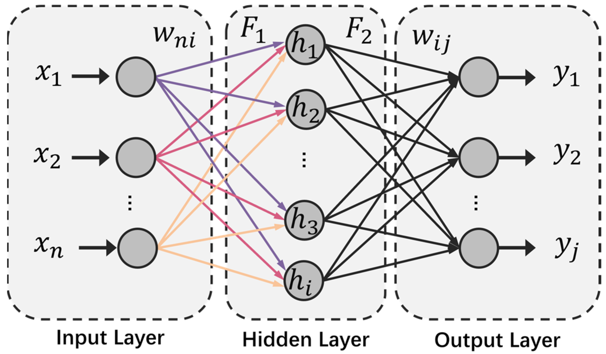
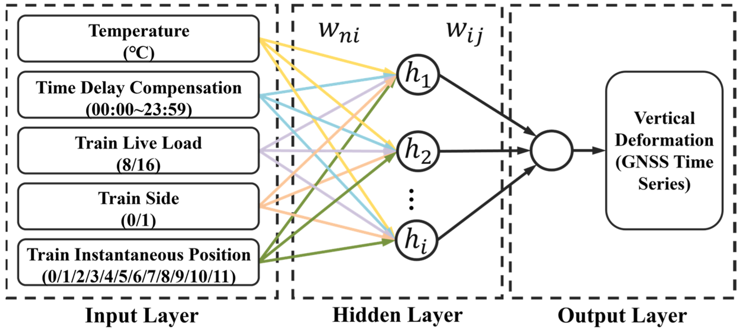
    The BP neural network structure is shown in Figure 2 and has three layers: the input, hidden, and output layers. The BP algorithm consists of two parts: forward propagation of information and backpropagation of errors, in which the input ( x 1 , x 2 , , x n ) is calculated from the input layer to the output layer ( y 1 , y 2 , , y j ) through the hidden layer based on the activation function ( F 1 , F 2 ). If the desired output is not obtained in the output layer, the error change in the output layer is calculated. Subsequently, backpropagation through the network returns the error signal along the original connection path to modify the weight ( w n i , w i j ) of each layer of neurons until the desired goal is achieved.
  • BP neural network prediction: A total of 20% of the sample set was used as the test set, which was input into the trained BP neural network. The predicted results were then normalized.
  • Analysis of the prediction effect in terms of performance metrics. A factor selection model was used to compare the contributions of each factor to the prediction. Neural network comparison experiments were then used to analyze BP prediction ability. In all the prediction effect analyses, we used the residual e , MAE, and MRE. The MAE, MRE, and coefficient of determination (R2) were calculated to evaluate the prediction accuracy of the proposed model [15]. According to the MRE and MAE criteria, the smaller the value, the more accurate the model, indicating a higher prediction accuracy. For a group of measurement data x 1 , x 2 , , x n , the MAE formula (Equation (2)), the MRE formula (Equation (3)), and R2 (Equation (4)) are as follows, respectively:
M A E = 1 n i = 1 n x i x i ^ ,
M R E = 1 n i = 1 n x i x i ^ x i × 100 % ,
R 2 = 1 i = 1 n x i x i ^ 2 i = 1 n x i x ¯ 2 ,
where x i ^ is the predicted value, x i is the measured value for i t h sample, x ¯ is the corresponding mean test value, and n is the number of samples in the test dataset.

3. Background for a Study Case

3.1. Bridge Description

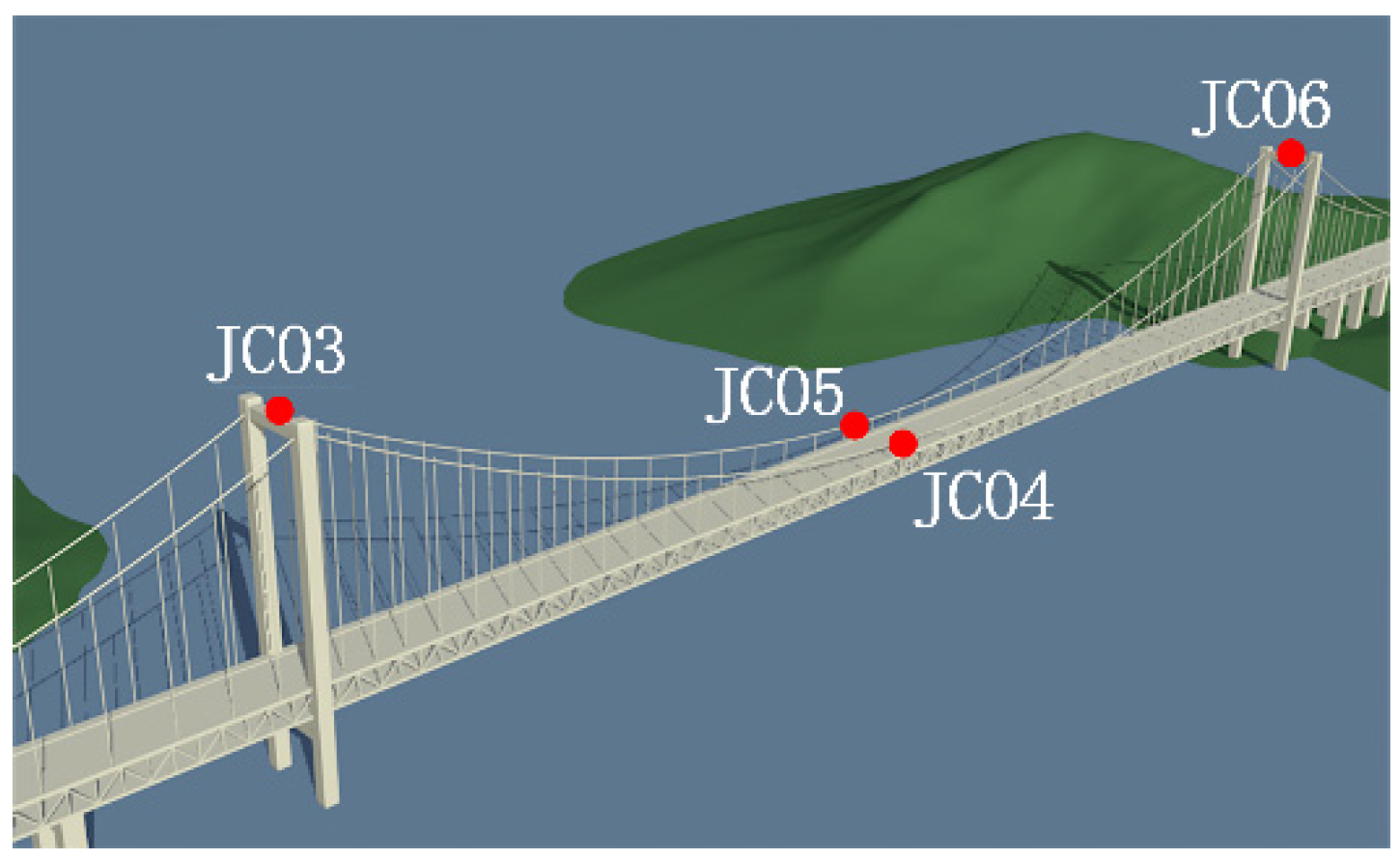
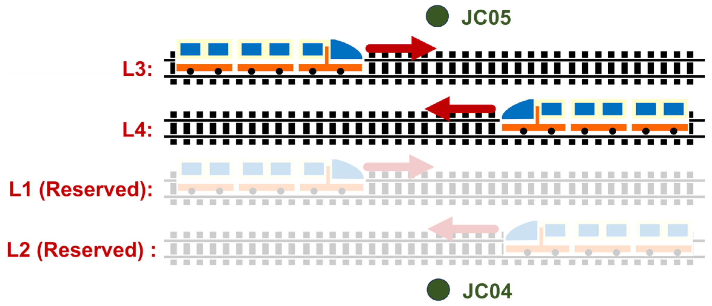
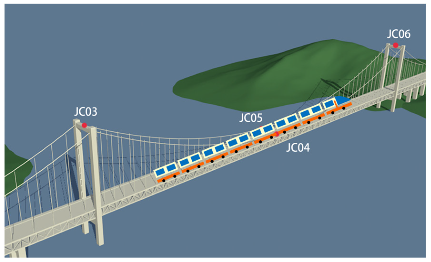
In this section, we consider the case of an HSRSB. The studied bridge opened in December 2020. This HSRSB was symmetrical to its centerline, with a span layout of 84 + 84 + 1092 + 84 + 84 m (Figure 3). The upper bridge deck has eight lanes with a maximum speed of 100 km/h. The lower deck is arranged using four high-speed railways (Figure 4). The direction of the four railways (tracks) is shown in Figure 5. The four railways (tracks) are marked L1 (reserved), L2 (reserved), L3, and L4. The design speed of the corresponding train is 380 km/h when running on the land track and 250 km/h when running on the HSRSB. Based on the HSRSB design requirements, a high-speed train with a total length of 438.4 m was used. The HSRSB has high ride stability and comfort requirements. The 1092 m main span and total floating system lead to high flexibility and low damping of the structure, which is subject to large vertical deformation under multiple loads [7].

3.2. Monitoring Scheme in the Field

Vertical deformation was measured using GNSS sensors. The HSRSB has six GNSS monitoring points, as shown in Figure 3. The reference station was located on the roof of the monitoring room (not shown). The monitoring points were arranged as follows: JC01 was at the upstream side anchorage (not shown); JC02 was downstream of the side anchorage (not shown); JC03 was at the top of tower No. 3; JC06 was at the top of tower No. 4; JC04 was upstream of the midspan; and JC05 was downstream of the midspan. During a train’s passage over a bridge, the midspan is the location where the stress and structural response of the main beam are the largest [1]. Therefore, only JC04 and JC05 data were used. The vertical direction exhibited the most significant response to load; therefore, only the vertical time series was used [35]. Only the vertical time series of sensors JC04 and JC05 were used. The sensors JC01, JC02, JC03, and JC06 were not used in this study.
The ambient temperature from the meteorological station was recorded by the temperature meters. Temperature meters were installed on the shore to measure air temperature via point measurements.

3.3. Characteristics of the Monitoring Data

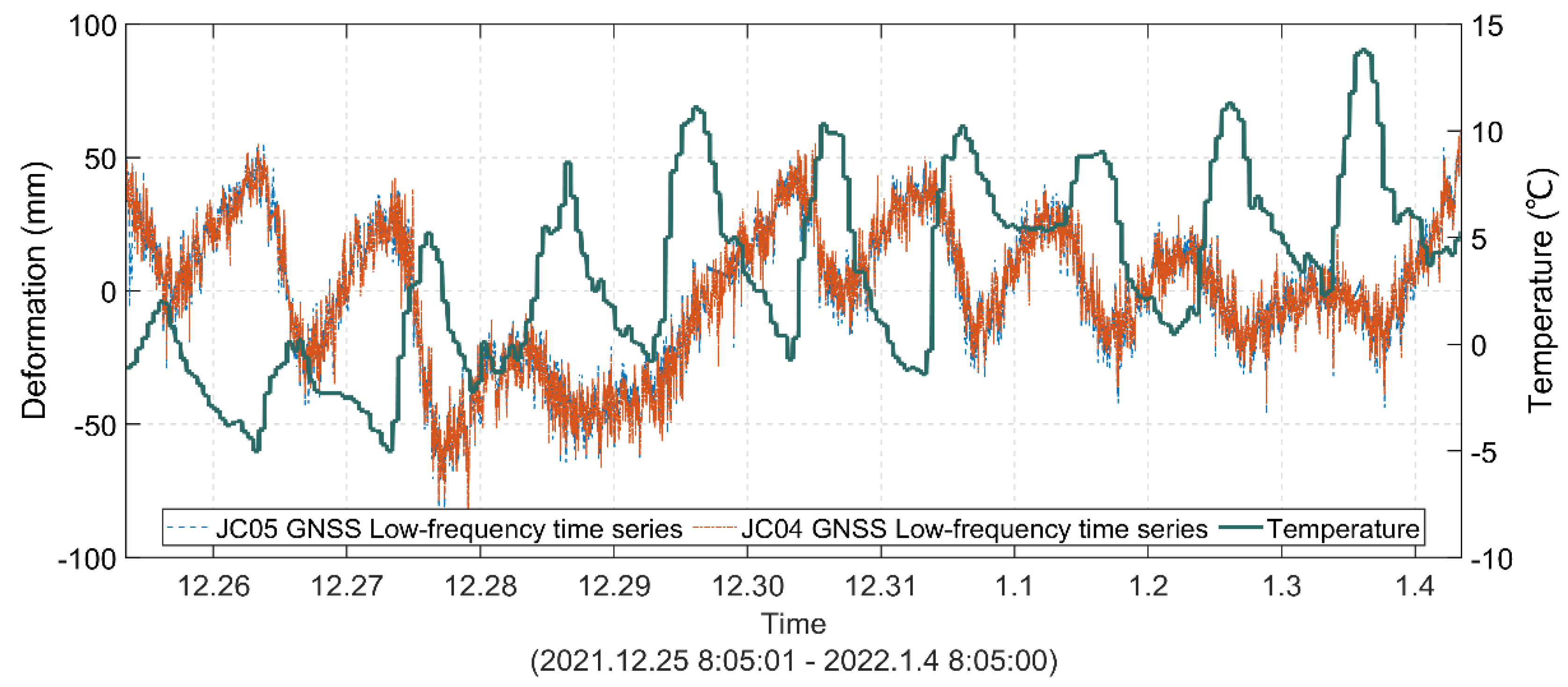
The 10-day vertical time series from 00:05:01 on 25 December 2021 to 00:05:00 on 4 January 2022 was selected. The sampling rate for the GNSS monitoring data was 1 Hz. The vertical accuracy was 8~9 mm. It is evident from Figure 6 and Figure 7 that the train live load and temperature significantly contribute to vertical deformation. We also determined the low-frequency trends of the deformation, which are shown as blue and orange lines in Figure 7. In the original data, the temperature significantly contributed to the low frequency (Figure 7). A high-frequency signal represents the train-induced deformation, which fluctuates with the temperature-induced deformation trend and resembles a spike (Figure 6).
We also monitored the temperature during the same period. The sampling interval of the installed thermometers was 1 h. Considering that temperature changes occur slowly, it is reasonable to use the hourly average temperature to demonstrate temperature variations [36,37]. The low frequency of the deformation was extracted and compared to the temperature. It can be gleaned from Figure 7 that there are diurnal cyclic variations in environmental temperature and low-frequency deformation. There is a strong correlation between the temperature and the deformation of the bridge. Over these 10 days, the temperature difference was 18.8 °C. The lowest temperature generally appears at 6–8 o’clock, and the highest temperature appears at 12–16 o’clock.

4. Results

4.1. Model Parameter Selection Strategy

The GNSS and temperature field data were used in the model parameter selection strategy. The GNSS data were subjected to a careful procedure to ensure that they could be used to monitor bridge deformation. The RTKLIB R2023a software, commonly used in GNSS data processing, was used for GNSS data resolution. Additionally, the GNSS time series was obtained using the dynamic solution mode, which is usually used when the monitoring point is on a moving carrier. The GNSS time series were preprocessed as follows: (i). All the missing epochs in the GNSS time series were filled using interpolation. The missing rate of the JC04 data was 0.31%, and that of JC05 was 0.44%, both of which are very small. (ii). Furthermore, distinct gross errors were removed from the time series.
In the following sections, the temperature and GNSS data are used to analyze the load response of the HSRSB, and it is concluded that TEMP, TDC, TLL, TS, and TIP are factors influencing vertical deformation.

4.1.1. Temperature, Time Delay Compensation, and Their Correlation with Vertical Deformation

Based on the field data, the relationship between vertical deformation and the temperature was analyzed. The low-frequency time series of the vertical deformation (blue and orange lines in Figure 7) was treated using low-pass filtering and compared with the temperature data (green lines in Figure 7). There was a negative correlation between the temperature and deformation. Cable temperature plays the dominant role. The main-span cable elongates due to the increase in its own temperature, which reduces its tension force and leads to the movement of the mid-span elevation of the girder [38]. The temperature fluctuation range is −5 °C~13.8 °C. The low-frequency vertical deformation range is −80 mm~60 mm.
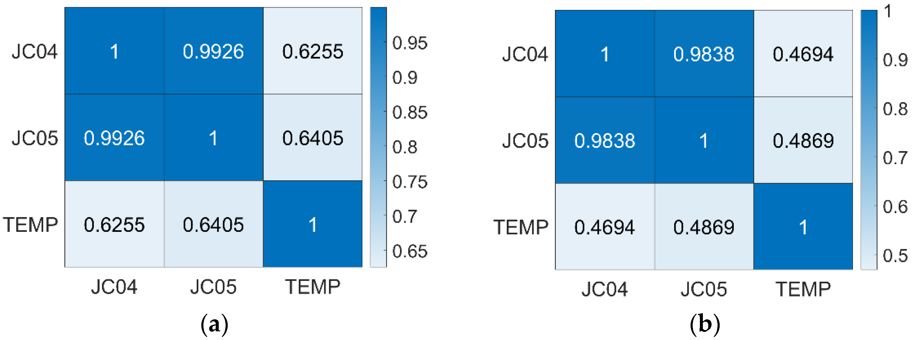
A quantitative correlation analysis comparing the temperature and vertical deformation is beneficial for understanding their relationships. Owing to the abnormal change in vertical deformation from 8:05:01 on 29 December 2021 to 8:05:00 on 30 December 2021, for which a reason is unknown, a correlation analysis was not carried out for this period, and a correlation analysis was carried out for the two time series, using this period as the dividing line. At this stage, the temperature data were multiplied by −1 to offset their negative correlation effect. The results of the correlation analyses are shown in Figure 8. JC04 and JC05 were highly correlated, with correlation coefficients of 0.99 and 0.98, respectively. The correlation coefficients between JC04 and temperature were 0.63 on 25 December 2021 at 8:05:01~29 December 2021 at 8:05:00 and 0.47 on 30 December 2021 at 8:05:01~4 January 2021 at 8:05:00. The correlation coefficients between JC05 and the temperature were 0.64 on 25 December 2021 at 8:05:01~29 December 2021 at 8:05:00 and 0.49 on 30 December 2021 at 8:05:01~4 January 2021 at 8:05:00. All correlation coefficients show that vertical deformation has a correlation with the temperature.
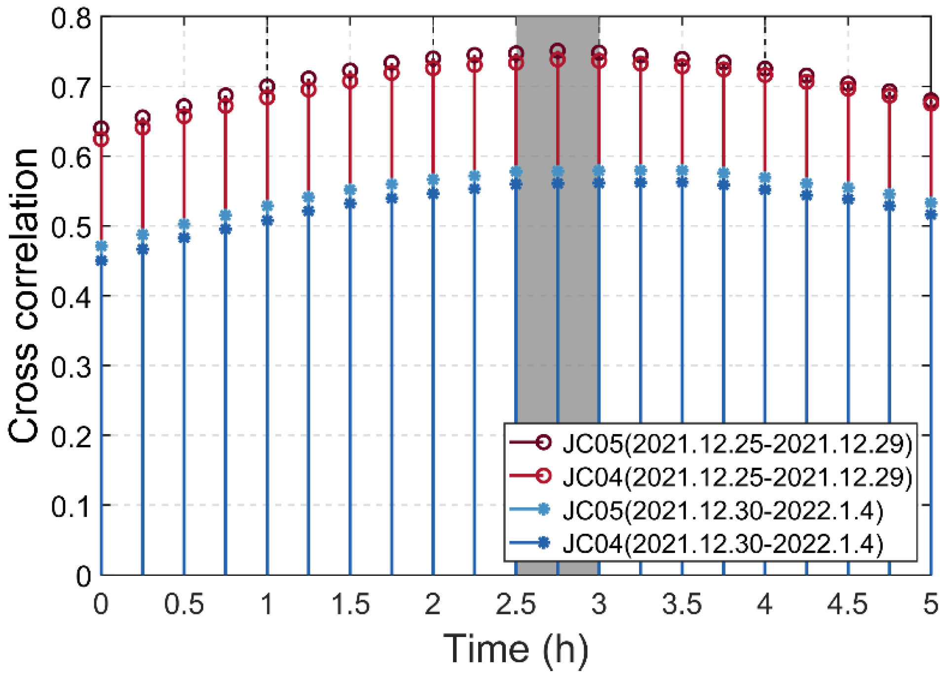
Owing to the slow heat conduction in the concrete structure, the internal temperature of the structure lagged behind the ambient temperature, resulting in a time lag between the vertical deformation and the ambient temperature. A cross-correlation analysis of the GNSS time series and temperature data under normalized conditions was carried out. The results are presented in Figure 9. In the 0~2.5 h interval, as the GNSS time series moved backward, the cross-correlation improved. In the 2.5~3 h interval, the cross-correlations reached their maximum. In the the data framed by the grey box, the peak cross-correlations of the four time series are 0.75 (purple), 0.74 (red), 0.58 (light blue), and 0.56 (dark blue). These results indicate that a temperature delay affects vertical deformation.
According to the results of the comparative and correlation analyses, the temperature and temperature delays are clearly related to vertical deformation. The TEMP and TDC were objectively identified as the factors influencing vertical deformation.

4.1.2. Train Live Load, Train Side, and Their Correlations with Vertical Deformation

To analyze the relationship between the deformation and train live load of the HSRSB, the deformation was processed via high-pass filtering to eliminate the influence of the temperature on vertical deformation. Based on the similar spike deformation characteristics caused by the train load, the time series of the train-passing time was intercepted. The train passed over the bridge 1020 times over 10 days. A maximum vertical deformation for 1020 times was considered for the analysis.
Typically, it is difficult to determine whether a train passes the upstream or downstream side every time. Fortunately, the HSRSB opened only at L3 and L4, providing a verifiable basis for grouping the operating sides. Among the four tracks, L1 and L2 are reserved lines, and L3 and L4 are open to traffic; that is, the downstream side (JC05) is open to traffic, and the upstream side (JC04) is not open. Therefore, the vertical deformation at JC05 was greater than that at JC04 when each train passed over (Figure 7). The trains include 8-car trains and 16-car trains. The normal distribution fitting for four cases of maximum vertical deformation should be analyzed: (i) JC04 monitored 8-car trains passing over the bridge; (ii) JC05 monitored 8-car trains passing over the bridge; (iii) JC04 monitored 16-car trains passing over the bridge; and (iv) JC05 monitored 16-car trains passing over the bridge.
According to the fitting results (Figure 10), the following conclusions can be drawn: (i) The statistical data for the four cases are highly consistent with a normal distribution. (ii) Due to the larger quantity of data in the eight-car train sets, their distribution is closer to a normal distribution. (iii) The maximum vertical deformation of JC05 is generally greater than that of JC04. (iv) The maximum vertical deformation induced by a 16-car train is generally greater than that caused by an 8-car train, although this is affected by the passenger volume inside the train. (v) The variances of the fitting results of the four cases are 15.69 mm, 13.15 mm, 11.96 mm, and 11.01 mm from left to right, respectively. There are two main reasons for this finding. First, the live load of each train is different, including vehicle load and passenger volume. Second, the vertical measurement accuracy of the GNSS time series using the dynamic solution mode was 8–9 mm. This also shows that the inner coincidence precision of 11–15 mm based on repeated measurements is consistent with the inner coincidence precision of 8–9 mm based on the GNSS solution results.

4.1.3. Train Instantaneous Position and Its Correlation with Vertical Deformation

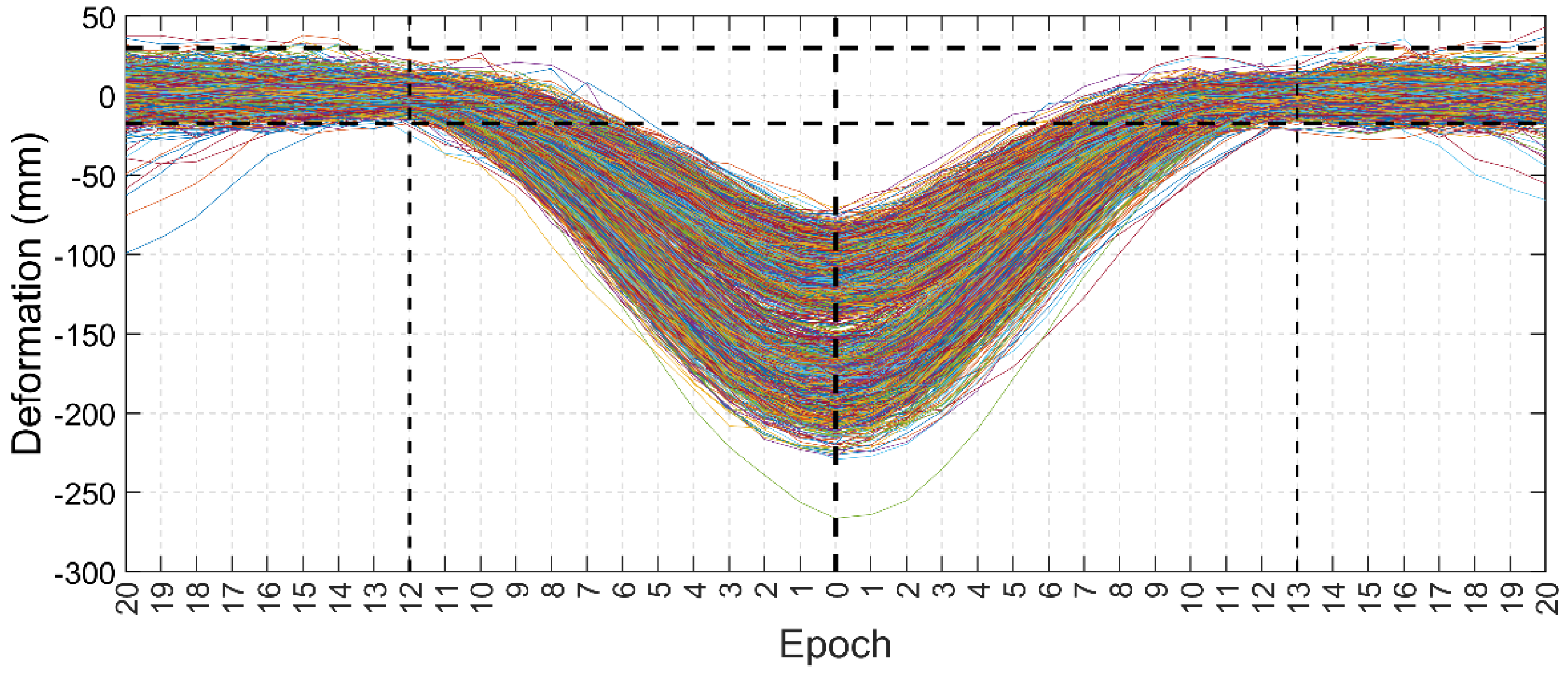
The relationship between the vertical deformation of the HSRSB and the instantaneous position of a train was analyzed. As shown in Figure 11, based on the epoch (corresponding to 1020 times) in which the maximum vertical deformation was located, 20 epochs were simulated before and after, constituting a total of 41 epochs. Except for a few special cases, train-induced vertical deformation was observed in epochs 12–13 before and after the maximum vertical deformation value was reached. When the train was at the midspan, the degree of vertical deformation was the largest. When the train left the midspan within 11 epochs, the vertical deformation gradually decreased. This means that a single complete passage of a train over the bridge usually generates a significant deformation of the bridge within 24–26 s. Additionally, the actual speed of the train is usually 151.2 km/h~163.8 km/h when running on this HSRSB.
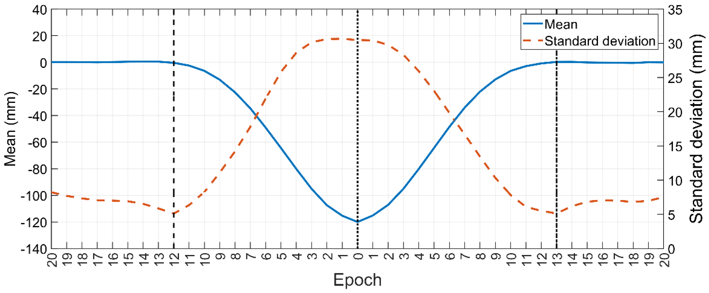
Although a preliminary conclusion is beneficial for understanding the train-induced deformation, it is still insufficient for high-precision predictions in practical applications. A more detailed quantitative analysis is required. To avoid oversampling, only the epochs with a strong correlation with deformation were used. All deformations of a single epoch in the 41 epochs were formed into a time series corresponding to said epoch, and a total of 41 time series were obtained. The mean and standard deviation of the 41 time series were calculated and plotted (Figure 12). In the left 20 → 12 intervals, the mean value is basically 0 because the train has not yet been on the bridge or the train load has little effect on mid-span deformation. During this period, the standard deviation gradually decreased within 5–8 mm, indicating that the distribution of the deformation values gradually became concentrated. This finding indicates that the train load gradually becomes the dominant load as the train moves towards the middle of the span; that is, vertical downward deformation occurs gradually. In the 12 → 0 section on the left side, the mean vertical deformation decreases with the increase in the train load, and the standard deviation increases gradually. This is because the TLL and TS generated by the 8-section marshalling train and 16-section marshalling trains become the dominant factors affecting bridge deformation. Since the correlation between deformation and TLL and TS is small at positions 20, 19, 18, 17, 16, 15, 14, 13, and 12, the MCD model is not applicable. Therefore, only data within 11 epochs of the training position were considered.
According to our analysis, TIP was significantly correlated with the vertical deformation. Therefore, TIP was considered an influencing factor of vertical deformation, and its MCD model input parameters were also determined.
In the model parameter selection strategy, five factors contributing to the vertical deformation of the HSRSB were objectively determined: TEMP, TDC, TLL, TS, and TIP. They were used as MCD model inputs to predict the vertical deformation.

4.2. MCD Prediction Model

4.2.1. MCD Prediction Model Data

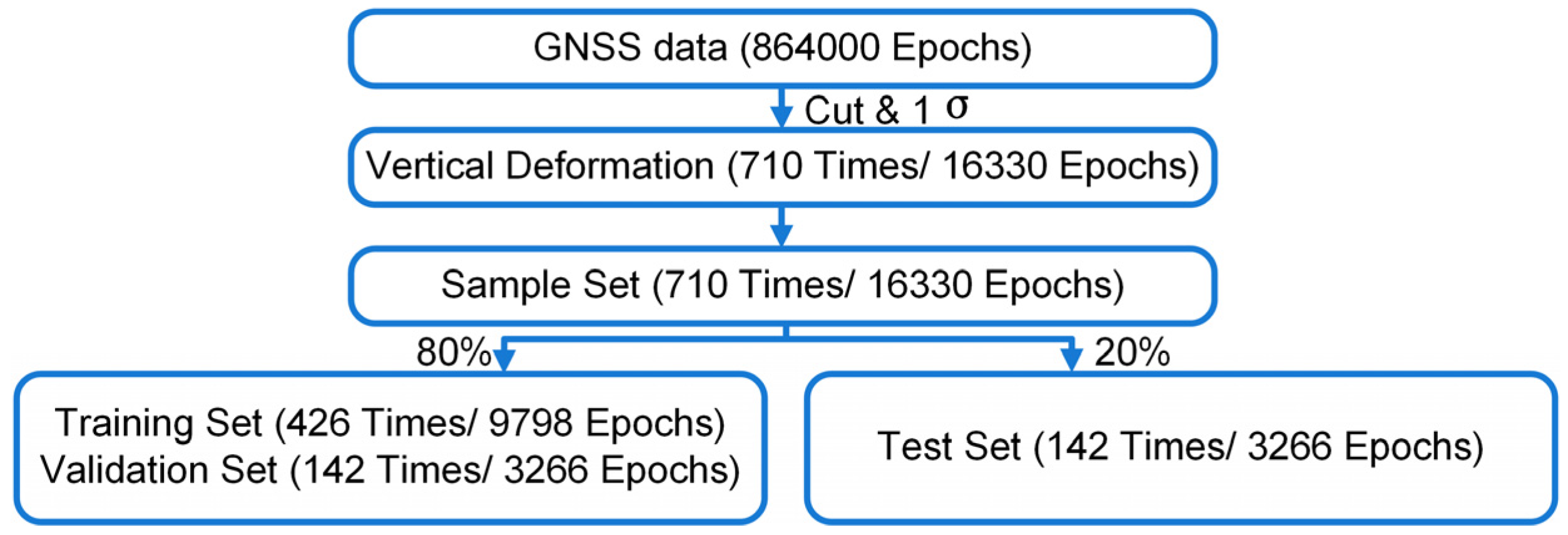
Machine learning accuracy is highly dependent on the dataset used. Therefore, reasonable, representative, and highly correlated data must be obtained. As shown in Figure 13, the MCD prediction model uses 10-day 1 Hz GNSS vertical deformation data, with a total of 864,000 epochs. During these 10 d, the trains passed over the bridge 1020 times for 23 epochs each time. Thus, 23,460 epochs were intercepted. In order to avoid data redundancy, we eliminated TLL fault classification results and extreme cases, and 1σ was used based on the normal distribution to further clean the data. The corresponding number of samples was 710 times (16,330 epochs), which were used as the sample set. Sixty percent of the sample set (426 times, 9798 epochs in total) was used as the training set. Twenty percent of the sample set (142 times, 3266 epochs in total) was used as the validation set. Twenty percent of the sample set (142 times, 3266 epochs in total) was used as the test set. The TEMP, TDC, TLL, TS, TIP, and vertical deformations of the same epoch were used as a set of data. In total, 13,064 sets of data were involved in the training. This sample size was sufficient to ensure the training effectiveness of the BP neural network. A total of 3266 sets of data were included in the prediction. The sample size was sufficient to verify the method, and the statistical results based on a large quantity of data had very high reference values.

4.2.2. BP Neural Network Architecture

The structure of the BP neural network is shown in Figure 14.
1.
BP input layer
A unified sampling rate was used in the first step. The temperature data were sampled hourly. However, the sampling rates of TEMP and TDC should be the same as the sampling rate of vertical deformation (1 Hz). Therefore, the temperature of the first epoch in each hour was taken as the value of 3600 epochs. Because the sampling rates of TLL, TS, and TIP are the same as those of vertical deformation, it was not necessary to resample them.
The second step involved determining the parameters for each model input. The TDC uses hourly and minute data as the BP input. The TLL was divided into two sets: an 8-car train and a 16-car train. TS was divided into two sets: trained and non-trained. For modeling, the 8-car and 16-car trains were transformed into the numerical values 8 and 16, and the train and non-train sides were transformed into the numerical values 0 and 1, respectively. Subsequently, we set the state of the train at the midspan (as shown in Figure 15) to 0. Based on the epochs required for the train to reach the midspan, we set 12 states (0, 1, 2, 3, 4, 5, 6, 7, 8, 9, 10, and 11). Additionally, a brief calculation formula for similar cases was derived.
t = l 2 v a ,
v is the train speed (m/s), l is the main span of the bridge (m), and a is a constant (1 or 2).
2.
BP hidden layer
The performance of a BP neural network depends on the corresponding parameters. This factor determines the accuracy of the prediction model. The quantities of nodes in the input layer n, hidden layer m, and output layer were all set to optimal values, where n = 5, m = 1, and output layer = 1. The size of the hidden layer was 7. The maximum number of training iterations was set to 100. The learning rate was set to 0.01. The minimum error for the training target was 0.00001. The hidden layer activation function was ‘tansig.’ The output layer activation function was ‘purelin’. The neural network learning training function was ‘trainlm’. The weight learning function was ‘learngdm’.

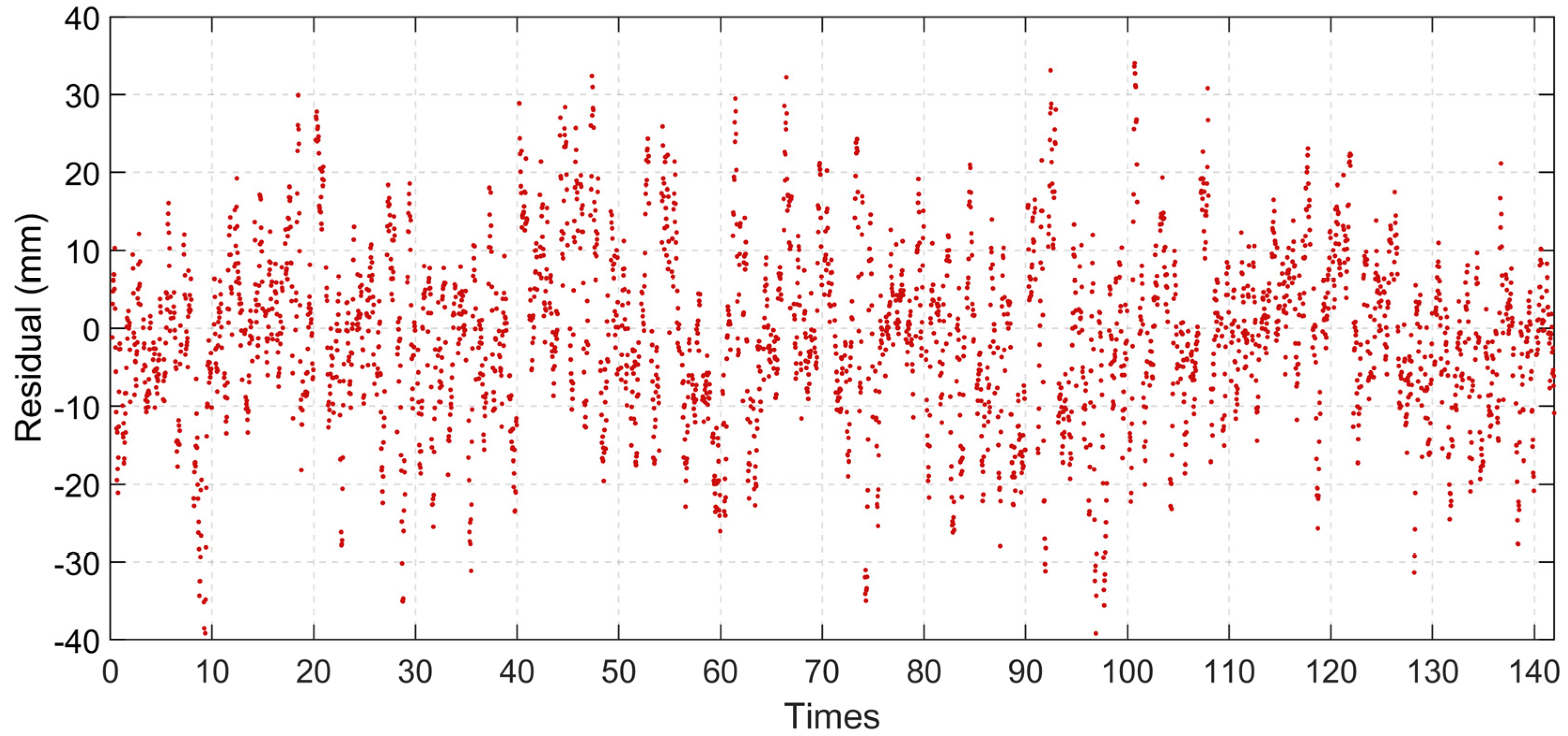
4.3. Experimental Results

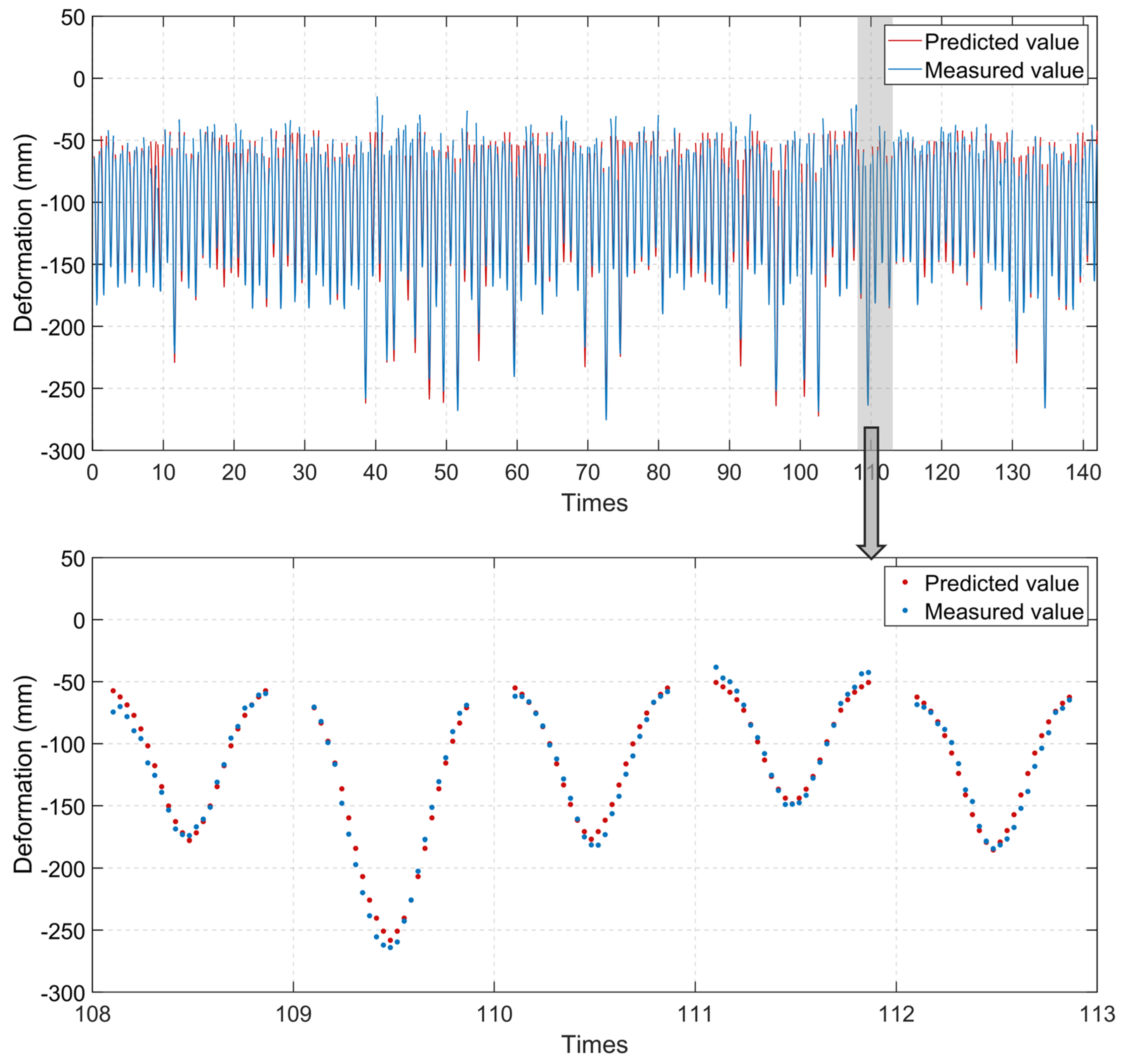
A comparison between the results predicted by the MCD prediction model and the measured values is shown in Figure 16, and the residuals are shown in Figure 17. The predicted values are consistent with the measured values. The prediction accuracy of the 8-car train is better than that of the 16-car train. Among the 142 crossings, there were 122 crossings of 8-car trains; the MAE was 8.48 mm, the MRE was 9.98%, and the R2 was 0.94. There were 20 crossings of 16-car trains; the MAE was 10.87 mm, the MRE was 8.85%, and the R2 is 0.94. The prediction residual MAE is 8.81 mm, the MRE is 9.82%, and the R2 was 0.94, indicating that the proposed model has a good fit and prediction accuracy. Under the limitations of GNSS vertical deformation accuracy (8–9 mm), the prediction results indicate that the MCD model captured almost all the factors influencing the HSRSB’s vertical deformation.
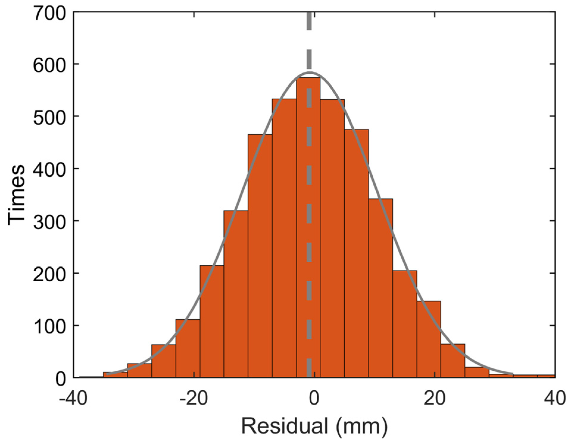
The results of the statistical analysis of the residuals are presented in Figure 18. The residual distribution is highly consistent with the normal distribution, indicating that the set is sufficient. The fitting result of the normal distribution shows that the mean is −0.44 mm, and the variance is 11.27 mm. This result shows that, with sufficient information to construct the model, the MCD prediction model may have a better prediction performance. There was no systematic deviation in the residual, and the distribution was concentrated. Therefore, the residual distribution results verify the effectiveness of the MCD prediction model. The residual distribution results obtained from sufficient data were statistically significant. This finding has significance as a reference for predicting the vertical deformation of HSRSBs.
To determine the separate contributions of the five influencing factors to the prediction accuracy, factor selection model comparative experiments were carried out. The factor selection model was set as follows: one, two, three, or four of the five influencing factors were removed. The MRE, MAE, R2, and improvement rate of the predicted results were used as evaluation indices to compare the contributions of the five influencing factors. The improvement rate was calculated using the following formula: (MAR of the predicted results after removing influencing factors − MAR of the predicted results using all influencing factors)/(MAR of the predicted results by remove influencing factors) × 100 (%). The results are shown in Table 1. ‘×’ means the influencing factor was removed. In comparison to the factor selection model, the MCD model aligns more closely with the measured vertical deformation, exhibiting a significantly higher prediction accuracy, with an improvement of up to 77.88%. Notably, when considering the three influencing factors of train live load, train side, and train instantaneous position, the improvement rate increases to 77.76%.
The residual error seems to be as high as 40 mm. This is not very good compared to the overall deformation range (250 mm). Figure 19 shows all the examples of records with high prediction errors (residual errors up to 30 mm). Prediction accuracy decreases when the deformation is unconventional. This may be due to the accidental effects of heavier vehicle loads. But the model still has good prediction results for the deformation trend.
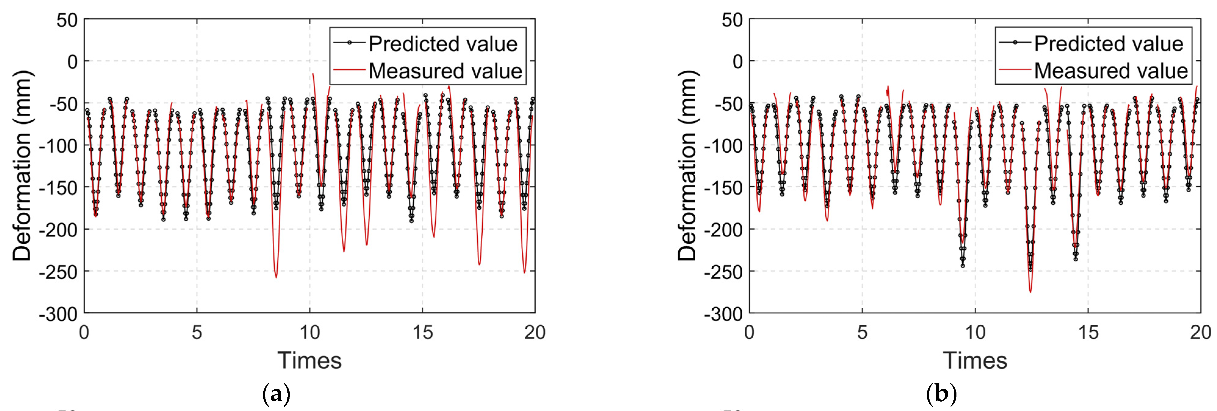
Without considering TLL, the model can predict the 8-car train formation, but the prediction accuracy of the 16-car train formation declines because there are too many data in the 8-car train sets to ignore the 16-car train sets (Figure 20a). Without considering TS, TEMP, or TDC, the model has no obvious deviation, but its prediction accuracy is significantly reduced (Figure 20b–d). In the case of TEMP and TDC, the temperature had no significant effect on the prediction. Because the selected sample data were taken from the data during the train-passing period, in these time series, the train live load was the dominant factor in the vertical deformation. The proportion of temperature factors during this period significantly reduced. However, for high-precision prediction, the influence of the temperature on displacement cannot be ignored; without considering TIP, the model cannot generate a prediction, and the predicted value can only represent the mean of this train passing over the bridge (Figure 20e).
To examine the suitability of the neural network model for the MCD model, commonly used prediction models were selected for comparison. These models include the Support Vector Machine (SVR), Radial Basis Function Neural Network (RBF), Recurrent Neural Network (RNN), and Long Short-Term Memory (LSTM). Experiments were conducted to determine the predictive capability of these models for HSRSBs. Table 2 presents the evaluation results for each prediction model. Because each model is suitable for prediction and the model input is sufficient for extracting deformation features for prediction, all the models have a good prediction ability. The BP model performed the best among all the models, with the lowest values of MRE and MAE. In addition, the CNN model had the best predictive capability among all the commonly used models. Compared to the LSTM model, the MAE of the BP model was 0.86 mm, and its MRE was 1.69%. Therefore, the BP model is reliable for predicting HSRSB deformation.

5. Discussion

Building upon the preceding experiment, the accuracy of deformation prediction primarily hinges on three key factors: methodology, model selection, and data quality. In the following sections, we delve into a comprehensive discussion of these factors and present practical approaches to enhancing prediction precision.
Method suitability: The prediction of vertical displacement methods can be categorized into three main groups: model-based methods, general formulas, and data-driven methods. Model-based approaches utilize finite element (FE) models for predictions. However, incorporating temperature changes into FE models poses a significant challenge. This method is employed on a case-by-case basis and exhibits limited generality. The development of general formulas relies heavily on extensive data collection and specialized expertise. In comparison to the preceding two approaches, data-driven methods are more adaptable for use across multiple bridges. Given that most long-span bridges are equipped with health-monitoring systems and ample data sources, machine learning has exhibited promise in the realm of displacement prediction.
Model completeness: Deformations in HSRSBs are highly intricate and difficult to predict accurately when relying on incomplete datasets. The reason why a prediction result of 8.82 mm was achieved using the MCD model can be attributed to the determination of influencing factors through the analysis of HSRSB load responses, thereby enhancing the comprehensiveness of the dataset. It is noteworthy that this study did not account for wind and vehicle loads. Typically, trains traverse a bridge within a brief 30 s timeframe, rendering the impact of wind loads on the bridge negligible during such a short duration. Furthermore, deformations induced by vehicle loads within the same 30 s timeframe are significantly smaller in magnitude compared to those caused by train loads. Nevertheless, optimizing the prediction model by considering potential contributions from vehicle and wind loads remains a viable avenue for further research.
Data quality: Superior results can be attained by improving data quality. In the case of GNSS data, significantly enhancing prediction accuracy remains challenging due to the inherent limitations of GNSS vertical accuracy. Simultaneously, a low sampling rate poses the risk of missing critical details pertaining to vertical deflection. The integration of GNSS with accelerometers offers the potential to not only augment data sampling rates but also enhance data accuracy. However, this avenue warrants further investigation. In this study, ambient temperatures were employed as the temperature data, which, in turn, contributed to a reduction in the prediction accuracy. Vertical deformation in a bridge results from a complex interplay of factors, including bridge beam temperature, tower temperature, cable temperature, temperature differentials between the beam’s top and bottom plates, etc. The development of more precise temperature modeling has the potential to further elevate the prediction accuracy. Nevertheless, this may concurrently introduce data redundancy.
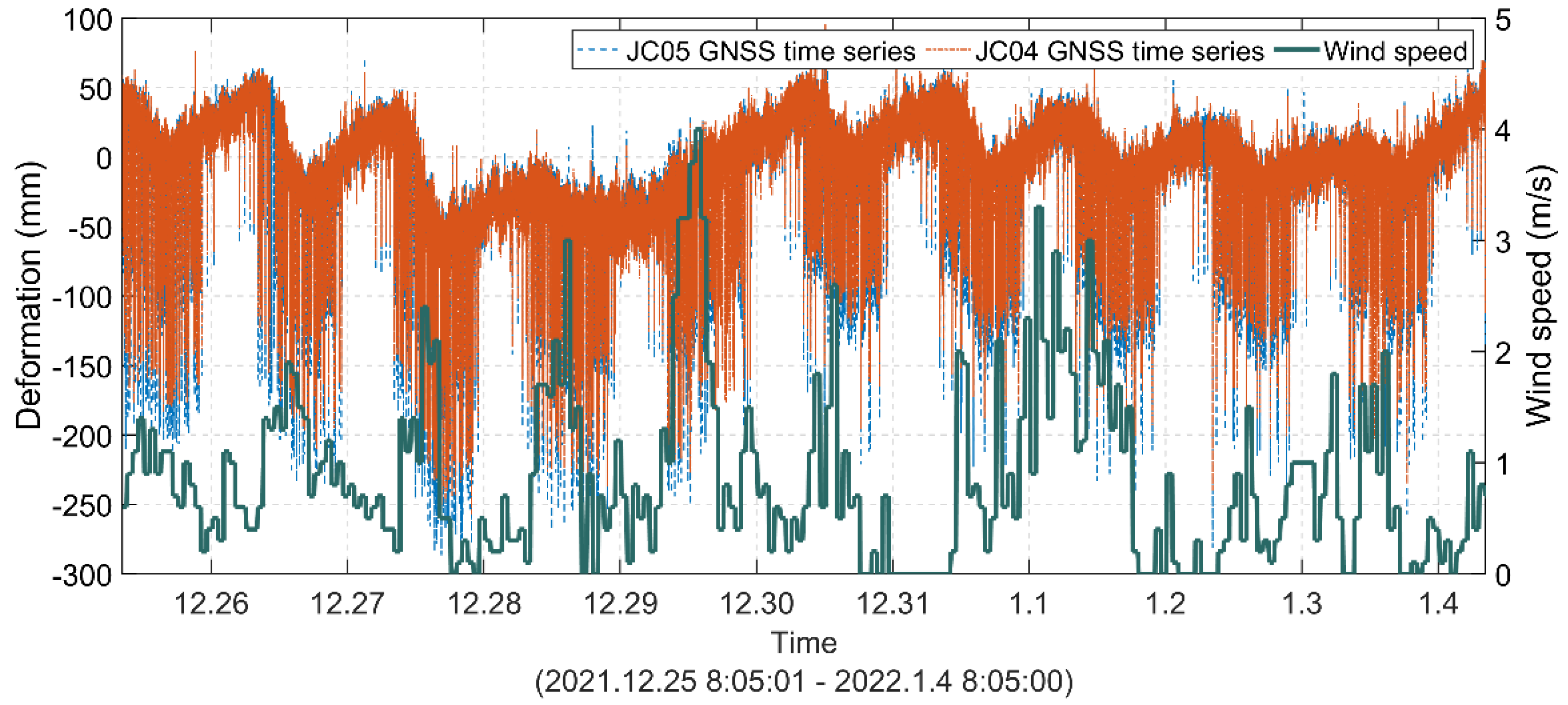
Wind and vehicle load also induced deformation. A comparison of wind speed and vertical deformation is presented in Figure 21. When wind speed is considered an influencing factor and used as a model input to predict deformation, the MAE is 8.81 mm, the MRE is 9.82%, the R2 is 0.94, and the improvement rate is almost 0. This is because December and January are not typhoon seasons; so, the wind speed is lower. High-wind speed data will benefit the research.
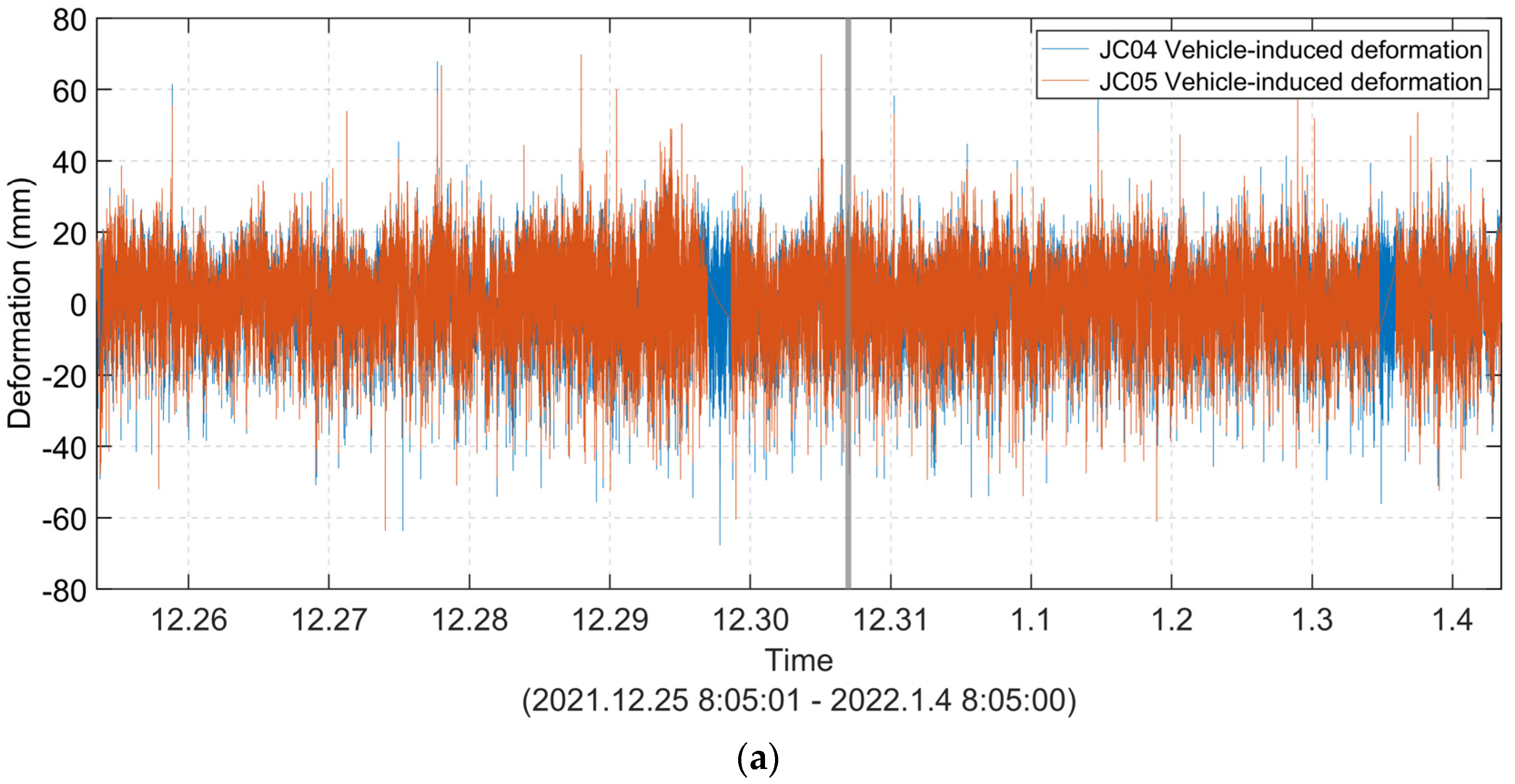
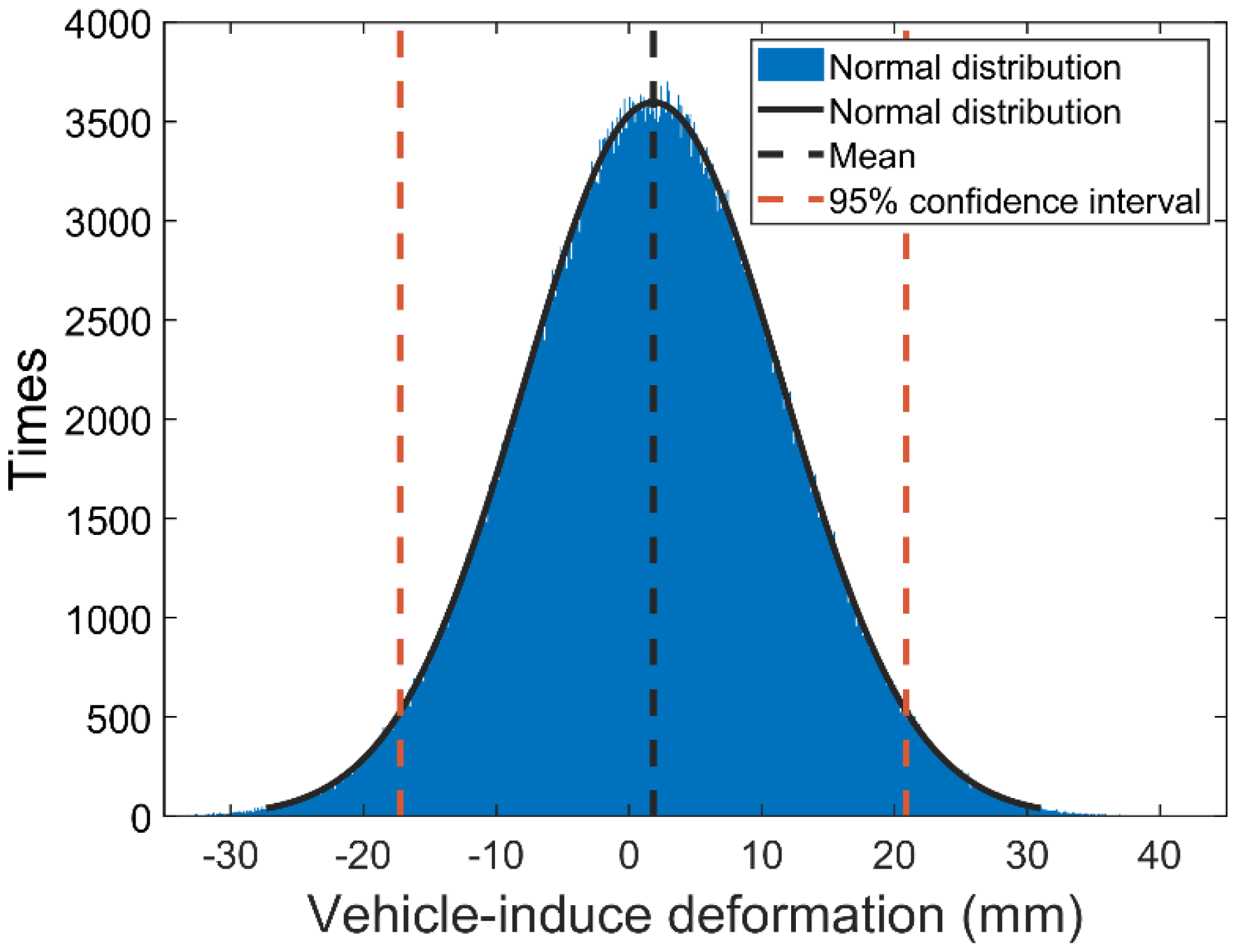
Since the 10-day data correspond to low-wind-speed conditions, the time series remaining after separating the train-induced deformation and the temperature-induced deformation can be considered to be vehicle-induced deformation (Figure 22). The statistical results for vehicle-induced deformation are shown in Figure 23. The variance was 9.73 mm, and the 95% probability of the distribution was less than 19.07 mm. As the bridge does not have a weighing system, it is difficult to predict deformation based on weight. The use of period statistics may be a feasible approach, but this requires long-term data. Further research will be conducted based on longer-period data.

6. Conclusions

In this study, we introduced a model parameter selection strategy for objectively identifying the factors influencing vertical deformation, which were subsequently utilized as inputs for the prediction model. Additionally, we presented a multi-load coupling deformation prediction model designed to forecast bridge deformation. To validate this model’s effectiveness, we selected a high-speed railway suspension bridge as our test case, and the results demonstrate a superior prediction accuracy. This means that, with the predicted temperature, when an 8/16-car train is traveling upstream/downstream, the prediction model can predict the bridge alignment in real time by dividing the bridge into 23 equal parts. This approach does not require the heavy workload of finite element modeling. The following conclusions can be drawn from our investigation:
  • Based on the load response analysis within the model parameter selection strategy of a high-speed railway suspension bridge, we conclude that vertical deformations result from a combination of five primary influencing factors: the temperature, time delay compensation, train live load, train side, and instantaneous train position.
  • The experimental results reveal a strong agreement between the predicted and measured values. The residual mean absolute error (MAE) was 8.81 mm, with a mean relative error (MRE) of 9.82% and a coefficient of determination (R2) of 0.94. These findings affirm the method’s capacity to accurately predict multifactor-coupled vertical deformations and nonlinear mapping relationships, further underscoring the suitability of the established multi-load coupling deformation model for vertical deformation prediction for high-speed railway suspension bridges.
  • In comparison to the factor selection model, the multi-load coupling deformation model aligns more closely with the measured vertical deformation, exhibiting a significantly higher prediction accuracy, with an improvement of up to 77.88%. Notably, when considering the three influencing factors of train live load, train side, and train instantaneous position, the improvement rate increases to 77.76%.
  • In the comparison experiments involving neural networks, all the models exhibited strong prediction capabilities due to the ample input data for extracting deformation features. The backpropagation (BP) neural network outperformed the other models.
  • This study contributes to the achievement of a comprehensive understanding of the behavior patterns exhibited by high-speed railway suspension bridges. The findings of this study hold significant importance in enhancing our comprehension of the structural stability of high-speed railway suspension bridges, offering valuable insights for future research endeavors.

Author Contributions

Conceptualization, S.L. and W.J.; methodology, W.J.; software, R.L.; validation, S.L. and X.T.; formal analysis, W.J.; investigation, X.T.; resources, Q.C. and R.L.; data curation, Q.C., J.W., and Z.Y.; writing—original draft preparation, S.L.; writing—review and editing, W.J.; supervision, J.W. and Z.Y. All authors have read and agreed to the published version of the manuscript.

Funding

This research was funded by the Major Science and Technology Program for Hubei Province under grant number 2022AAA002; the Innovative Research Group Project of the National Natural Science Foundation of China under grant number 41721003; and the National Natural Science Foundation of China under grant number 42004017.

Data Availability Statement

Data are unavailable due to privacy concerns.

Conflicts of Interest

Author Zhongtao Ye was employed by the company the China Railway Bridge Science Research Institute, Ltd. The remaining authors declare that the research was conducted in the absence of any commercial or financial relationships that could be construed as a potential conflict of interest.

References

  1. Li, W.J.; Gong, J.X.; Zhang, X.G. Study on live load reduction factors of train for long span mul-titrack railway suspension bridges. Structures 2021, 32, 1180–1191. [Google Scholar] [CrossRef]
  2. Xu, G.Y. Design of Long Span Railway Suspension Bridges; Shanghai Science and Technology Press: Shanghai, China, 2020; p. 14. (In Chinese) [Google Scholar]
  3. Li, Y.J. Current Situation and Expectation of Construction Technology for HSP Suspension Bridge with Kilometers Span. China Railw. 2019, 1–8. (In Chinese) [Google Scholar]
  4. Guo, H.; Su, P.F.; Zhao, X.X.; Liu, X.G.; Le, S.T. Displacement Characteristics at Girder End of Long Span Railway Suspension Bridge Under Design Loads. Railway Eng. 2019, 59, 14–19. (In Chinese) [Google Scholar]
  5. Tan, S.H.; Li, Z.W.; Shi, J.; Ma, D.K. Influence of Track Profile Setting on Dynamic Behavior of High-Speed Railway Suspension Bridge with Kilometer Span. China Railw. Sci. 2021, 42, 58–67. (In Chinese) [Google Scholar]
  6. Luo, J.F. Analysis of the Train Running Safety of Multi—Line Railway Cable—Stayed Bridge. J. Railw. Eng. Soc. 2018, 35, 58–62. (In Chinese) [Google Scholar]
  7. Zhao, K.Y.; Wang, H.; Gao, H. Antiseismic performance of the world’s first high-speed railway suspension bridge. J. Harbin Eng. Univ. 2021, 42, 1262–1270. (In Chinese) [Google Scholar]
  8. Zhang, W.M.; Lu, X.F.; Wang, Z.W.; Liu, Z. Effect of the main cable bending stiffness on flexural and torsional vibrations of suspension bridges: Analytical approach. Eng. Struct. 2021, 240, 112393. [Google Scholar] [CrossRef]
  9. Xu, X.; Ren, Y.; Huang, Q.; Fan, Z.Y.; Tong, Z.J.; Chang, W.J.; Liu, B. Anomaly detection for large span bridges during operational phase using structural health monitoring data. Smart Mater. Struct. 2020, 29, 045029. [Google Scholar] [CrossRef]
  10. Tang, H.Q.; Xu, G.Y.; Liu, H.S. Feasibility Analysis of Applying of Suspension Bridge Type to Railway Bridges. Bridge Constr. 2017, 47, 13–18. (In Chinese) [Google Scholar]
  11. Zhang, W.M.; Lu, X.F.; Chang, J.Q.; Tian, G.M. An Analytical Algorithm for Estimating the Deck’s Maximum Deflection and Deck-End Rotation Angle of a Suspension Bridge under Live Load. J. Bridge Eng. 2022, 27, 04022055. [Google Scholar] [CrossRef]
  12. Ding, Y.L.; Zhao, H.W.; Deng, L.; Li, A.Q.; Wang, M.Y. Early Warning of Abnormal Train-Induced Vibrations for a Steel-Truss Arch Railway Bridge: Case Study. J. Bridge Eng. 2017, 22, 05017011. [Google Scholar] [CrossRef]
  13. Fan, Z.; Huang, Q.; Ren, Y.; Xu, X.; Zhu, Z. Real-Time Dynamic Warning on Deflection Abnormity of Cable-Stayed Bridges Considering Operational Environment Variations. J. Perform. Constr. Facil. 2020, 35, 04020123. [Google Scholar] [CrossRef]
  14. He, Z.; Li, W.; Salehi, H.; Zhang, H.; Zhou, H.; Jiao, P. Integrated structural health monitoring in bridge engineering. Autom. Constr. 2022, 136, 104168. [Google Scholar] [CrossRef]
  15. Ye, X.W.; Sun, Z.; Lu, J. Prediction and early warning of wind-induced girder and tower vibration in cable-stayed bridges with machine learning-based approach. Eng. Struct. 2023, 275, 115261. [Google Scholar] [CrossRef]
  16. Lee, J.; Jeong, S.; Lee, J.; Sim, S.H.; Lee, K.C.; Lee, Y.J. Sensor data-based probabilistic monitoring of time-history deflections of railway bridges induced by high-speed trains. Struct. Health Monit. 2022, 21, 2518–2530. [Google Scholar] [CrossRef]
  17. Zhou, Y.; Sun, L.M. A comprehensive study of the thermal response of a long-span cable-stayed bridge: From monitoring phenomena to underlying mechanisms. Mech. Syst. Signal Process. 2019, 124, 330–348. [Google Scholar] [CrossRef]
  18. Meng, Q.L.; Zhu, J.S. Fine temperature effect analysis-based time-varying dynamic properties evaluation of long-span suspension bridges in natural environments. J. Bridge Eng. 2018, 23, 04018075. [Google Scholar] [CrossRef]
  19. Yang, K.; Ding, Y.; Sun, P.; Zhao, H.; Geng, F. Modeling of temperature time-lag effect for concrete box-girder bridges. Appl. Sci. 2019, 9, 3255. [Google Scholar] [CrossRef]
  20. Jiang, H.; Wan, C.; Yang, K.; Ding, Y.; Xue, S. Modeling relationships for field strain data under thermal effects using functional data analysis. Measurement 2021, 177, 109279. [Google Scholar] [CrossRef]
  21. Zhao, H.W.; Ding, Y.L.; Nagarajaiah, S.; Li, A.Q. Behavior Analysis and Early Warning of Girder Deflections of a Steel-Truss Arch Railway Bridge under the Effects of Temperature and Trains: Case Study. J. Bridge Eng. 2019, 24, 05018013. [Google Scholar] [CrossRef]
  22. Liu, J.B. Analysis of Global Static and Dynamic Property of Long-Span Steel Truss Girder Rail-cum-Road Suspension Bridge. Bridge Constr. 2020, 50, 23–28. (In Chinese) [Google Scholar]
  23. Zhou, Y.Z.; Chen, L.J.; Gao, C. Design Techniques and Exploration of High-Speed Railway Bridges in China. Bridge Constr. 2018, 48, 11–15. (In Chinese) [Google Scholar]
  24. Wang, H.; Ding, G.; Tang, H.; Chen, L.K. Numerical Seismic Analysis of Simply-Supported Girder Railway Bridge under High-Speed Train Load. Appl. Mech. Mater. 2011, 80–81, 566–570. [Google Scholar] [CrossRef]
  25. Lei, X.; Siringoringo, D.M.; Sun, Z.; Fujino, Y. Displacement response estimation of a cable-stayed bridge subjected to various loading conditions with one-dimensional residual convolutional autoencoder method. Struct. Health Monit. 2023, 22, 1790–1806. [Google Scholar] [CrossRef]
  26. Qin, S.Q.; Gao, Z.Y. Developments and prospects of long-span high-speed railway bridge technologies in China. Engineering 2017, 3, 787–794. [Google Scholar] [CrossRef]
  27. Fan, Q.; Meng, X.L.; Nguyen, D.T.; Xie, Y.; Yu, J. Predicting displacement of bridge based on CEEMDAN-KELM model using GNSS monitoring data. J. Appl. Geod. 2020, 14, 253–261. [Google Scholar] [CrossRef]
  28. Xu, Y.; Fenerci, A.; Øiseth, O.; Moan, T. Efficient prediction of wind and wave induced long-term extreme load effects of floating suspension bridges using artificial neural networks and support vector machines. Ocean Eng. 2020, 217, 107888. [Google Scholar] [CrossRef]
  29. Kang, F.; Li, J.; Zhao, S.; Wang, Y. Structural health monitoring of concrete dams using long-term air temperature for thermal effect simulation. Eng. Struct. 2019, 180, 642–653. [Google Scholar] [CrossRef]
  30. Gu, C.S.; Wu, B.Q.; Chen, Y.J. A High-robust displacement prediction model for super-high arch dams integrating wavelet de-noising and improved random forest. Water 2023, 15, 1271. [Google Scholar] [CrossRef]
  31. Chen, Q.; Jiang, W.; Meng, X.; Jiang, P.; Wang, K.; Xie, Y.; Ye, J. Vertical deformation monitoring of the suspension bridge tower using GNSS: A case study of the Forth Road Bridge in the UK. Remote Sens. 2018, 10, 364. [Google Scholar] [CrossRef]
  32. Tan, X.; Chen, W.; Tan, X.; Zou, T.; Du, B. Prediction for the future mechanical behavior of underwater shield tunnel fusing deep learning algorithm on SHM data. Tunn. Undergr. Space Technol. 2022, 125, 104504. [Google Scholar] [CrossRef]
  33. Tan, X.; Sun, X.; Chen, W.; Du, B.; Ye, J.; Sun, L. Investigation on the data augmentation using machine learning algorithms in structural health monitoring information. Struct. Health Monit. 2021, 20, 2054–2068. [Google Scholar] [CrossRef]
  34. Tan, X.; Chen, W.; Zou, T.; Yang, J.; Du, B. Real-time prediction of mechanical behaviors of underwater shield tunnel structure using machine learning method based on structural health monitoring data. J. Rock Mech. Geotech. Eng. 2023, 15, 886–896. [Google Scholar] [CrossRef]
  35. Zhao, K.Y.; Wang, H.; Tao, T.Y.; Gao, H.; Wu, T. Parametric analysis on buffeting performance of a long-span high-speed railway suspension bridge. J. Cent. South Univ. 2022, 29, 2574–2588. [Google Scholar] [CrossRef]
  36. Xu, X.; Huang, Q.; Ren, Y.; Zhao, D.Y.; Yang, J.; Zhang, D.Y. Modeling and separation of thermal effects from cable-stayed bridge response. J. Bridge Eng. 2019, 24, 04019028. [Google Scholar] [CrossRef]
  37. Zhou, Y.; Sun, L.M. Insights into temperature effects on structural deformation of a cable-stayed bridge based on structural health monitoring. Struct. Health Monit. 2018, 18, 778–791. [Google Scholar] [CrossRef]
  38. Zhou, Y.; Xia, Y.; Chen, B.; Fujino, Y. Analytical solution to temperature-induced deformation of suspension bridges. Mech. Syst. Signal Process. 2020, 139, 106568. [Google Scholar] [CrossRef]
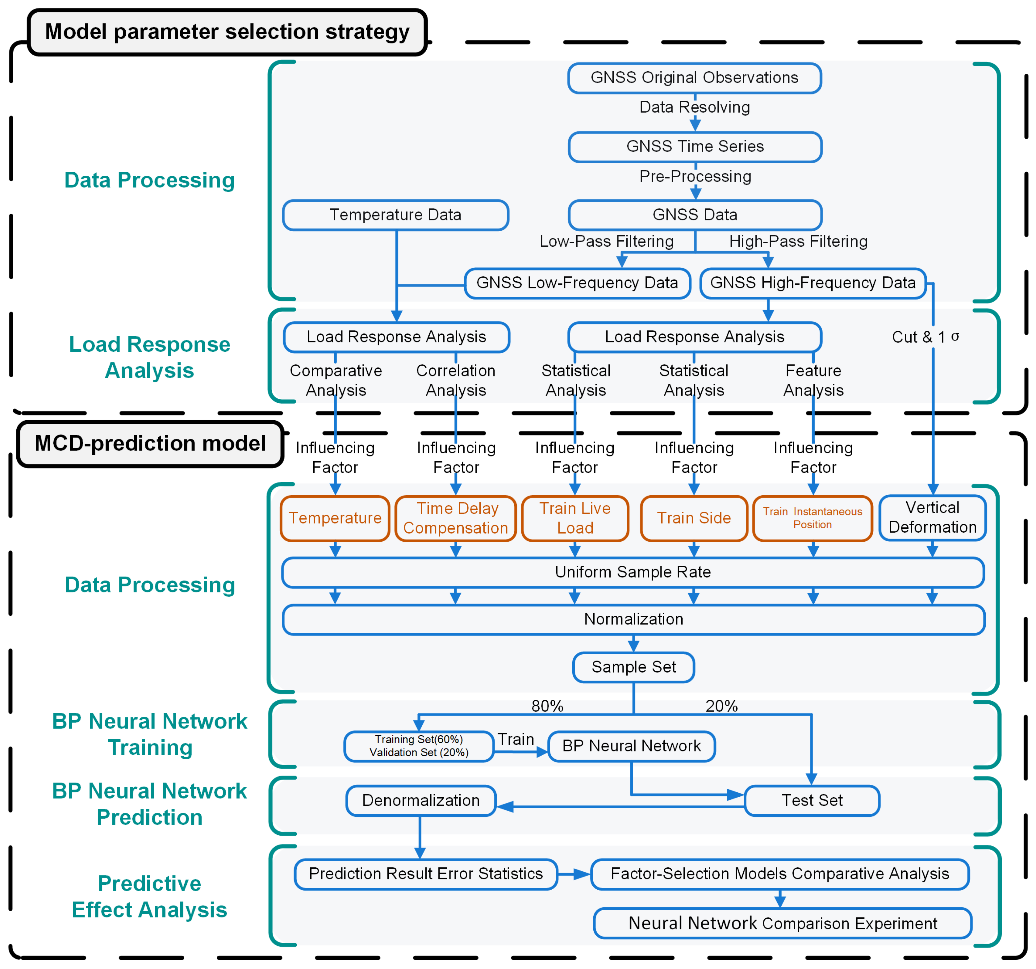
Figure 1. Flow chart of the experimental process.
Remotesensing 16 01687 g001
Figure 2. Radial basis function neural network structure.
Remotesensing 16 01687 g002
Figure 3. Monitoring points on the high-speed railway suspension bridge.
Remotesensing 16 01687 g003
Figure 4. High-speed railway suspension bridge cross-section.
Remotesensing 16 01687 g004
Figure 5. Four-line railway track.
Remotesensing 16 01687 g005
Figure 6. Ten-day vertical GNSS time series of the monitoring points at the mid-span of the high-speed railway suspension bridge. (a) Vertical GNSS time series. (b) Detailed view of the data framed by the grey box in subfigure (a) regarding the train live load, which significantly contributes to vertical deformation.
Remotesensing 16 01687 g006
Figure 7. Comparison of the temperature and low-frequency vertical deformation.
Remotesensing 16 01687 g007
Figure 8. Coefficient test matrix of the Pearson correlation analysis. (a) Data for 25 December 2021 8:05:01~29 December 2021 8:05:00. (b) Data for 30 December 2021 8:05:01~4 January 2021 8:05:00.
Remotesensing 16 01687 g008
Figure 9. Temperature time delay Pearson correlation analysis.
Remotesensing 16 01687 g009
Figure 10. Statistical diagram of the maximum vertical deformation caused by passing trains.
Remotesensing 16 01687 g010
Figure 11. Vertical deformation during train passage.
Remotesensing 16 01687 g011
Figure 12. Mean and standard deviation of the vertical deformation during train passage.
Remotesensing 16 01687 g012
Figure 13. Data flow.
Remotesensing 16 01687 g013
Figure 14. Structure of the BP neural network in the MCD prediction model.
Remotesensing 16 01687 g014
Figure 15. Considered state of the train at the midspan of the bridge.
Remotesensing 16 01687 g015
Figure 16. Comparison between the predicted and measured values.
Remotesensing 16 01687 g016
Figure 17. Residual between the predicted and measured vertical deformation values.
Remotesensing 16 01687 g017
Figure 18. Residual statistics and normal distribution.
Remotesensing 16 01687 g018
Figure 19. Predicted values with a residual greater than 30 mm.
Remotesensing 16 01687 g019
Figure 20. Comparison between the predicted and measured deformation values in factor selection model: (a) without considering TLL; (b) without considering TS; (c) without considering TEMP; (d) without considering TDC; and (e) without considering TIP.
Remotesensing 16 01687 g020aRemotesensing 16 01687 g020b
Figure 21. Comparison of wind speed and vertical deformation.
Remotesensing 16 01687 g021
Figure 22. 10-day vehicle-induced deformation of the monitoring points at the midspan of the high-speed railway suspension bridge: (a) vehicle-induced deformation; (b) detailed view of the data framed by the grey box in subfigure (a).
Remotesensing 16 01687 g022aRemotesensing 16 01687 g022b
Figure 23. Statistical diagram of vehicle-induced deformation.
Remotesensing 16 01687 g023
Table 1. The influence of the influencing factors on the prediction accuracy.
Influencing Factor Was RemovedMREMAE (mm)R2ImprovementRate
TLLTSTEMPTIPTDC
9.82%8.810.94/
× 14.59%15.280.7842.34%
× 11.69%11.070.9120.42%
× 10.37%9.180.944.03%
× 43.19%37.580.1876.56%
×11.34%9.880.9310.83%
×× 15.62%16.420.7546.35%
× × 14.46%15.080.7741.58%
× × 45.43%39.280.0477.57%
× ×15.76%15.910.7744.63%
×× 11.90%11.220.9121.48%
× × 44.01%37.930.1576.77%
× ×12.83%11.890.925.90%
×× 43.60%37.650.1776.60%
× ×11.56%10.050.9312.34%
××44.14%37.830.1676.71%
××× 15.87%16.560.7446.80%
×× × 45.85%39.610.0177.76%
×× ×16.69%170.7448.18%
× ×× 45.28%39.330.0377.60%
× × ×15.68%15.850.7744.42%
× ××45.51%39.330.0377.60%
××× 43.76%37.950.1576.79%
×× ×13.16%12.110.927.25%
× ××45.34%38.210.1476.94%
×××43.84%37.770.1676.67%
××××44.78%38.150.1476.91%
× ×××45.98%39.430.0377.66%
×× ××46.77%39.830.0177.88%
××× ×17.07%17.340.7449.19%
×××× 46.21%39.750.0177.84%
Table 2. Evaluation of five networks with different neural network architectures.
BPLSTMCNNRBFSVR
MRE9.82%11.51%11.99%11.65%13.52%
MAE (mm)8.819.679.8810.2412.04
R20.940.940.940.940.89
Disclaimer/Publisher’s Note: The statements, opinions and data contained in all publications are solely those of the individual author(s) and contributor(s) and not of MDPI and/or the editor(s). MDPI and/or the editor(s) disclaim responsibility for any injury to people or property resulting from any ideas, methods, instructions or products referred to in the content.