Abstract
The extraction of photovoltaic (PV) panels from remote sensing images is of great significance for estimating the power generation of solar photovoltaic systems and informing government decisions. The implementation of existing methods often struggles with complex background interference and confusion between the background and the PV panels. As a result, the completeness and edge clarity of PV panel extraction results are compromised. Moreover, most previous studies have overlooked the unique color characteristics of PV panels. To alleviate these deficiencies and limitations, a method for extracting photovoltaic panels from high-resolution optical remote sensing images guided by prior knowledge (PKGPVN) is proposed. Firstly, aiming to address the problems related to missed extractions and background misjudgments, a Photovoltaic Index (PVI) based on visible images in the three-band is constructed to serve as prior knowledge to differentiate between PV panels and non-PV panels. Secondly, in order to strengthen information interaction between shallow features and deep features and enhance the accuracy and integrity of results, a Residual Convolution Hybrid Attention Module (RCHAM) is introduced into the skip-connection of the encoding–decoding structure. Finally, for the purpose of reducing the phenomenon of blurred edges, a multilevel Feature Loss (FL) function is designed to monitor the prediction results at different scales. Comparative experiments are conducted with seven methods, including U-Net, on publicly available datasets. The experimental results show that our PKGPVN achieves superior performance in terms of evaluation metrics such as IoU (above 82%), Precision (above 91%), Recall (above 89%), and F1-score (above 90%) on the AIR-PV dataset. Additionally, the ablation experiments illustrate the effectiveness of our key parts. The proposed method reduces the phenomena of missed extractions and background misjudgments effectively while producing highly accurate results with clear boundaries.
1. Introduction
1.1. Background and Significance
Solar energy, as a green energy source, is experiencing a steady rise in its global energy utilization. Solar energy stands out as the most abundant natural source compared with other conventional energy sources, and it has the characteristics of high efficiency, environmental friendliness, and inexhaustibility [1]. With advancements in technology and increased government attention, photovoltaic (PV) power generation has gradually become one of the most promising low-carbon energy generation methods [2]. Against the backdrop of the increasing application rate and scope of PV panels, achieving the automated management of PV panels has become a practical industrial demand. The automatic, fast, and precise identification and extraction of PV panels is crucial for estimating photovoltaic power generation, analyzing regional distribution and dynamic change, and providing crucial data to support government decision making efforts.
The manual survey of PV panels offers the advantage of capturing specific information, such as number, color, texture, inclination, and direction angle. However, the drawbacks are laborious, time-consuming, inefficient, and easily limited by the environment. In contrast, remote sensing technology has the advantages of being efficient, wide-ranging, and low-cost. Therefore, the precise identification and extraction of PV panels through remote sensing technology has become a research hotspot. According to the different sensor platforms, remote sensing can be roughly categorized into ground-based remote sensing, aerial remote sensing, and space-based remote sensing.
1.2. Current Methods
In recent years, both domestic and international scholars have conducted extensive research on the extraction of PV panels based on remote sensing images. The existing methods mainly fall into two categories: traditional image-processing-based methods and deep learning-based methods. Traditional methods include segmentation-based approaches, such as color-based segmentation. This method detects PV panels based on their shape as prior knowledge [3]. Traditional methods also include supervised classification-based approaches, where the Support Vector Machine (SVM) classifier [4] or Random Forest (RF) classifier [5] is used to assign corresponding categories to each pixel in the image, followed by post-processing to identify the PV panel areas. Chen et al. [6] made an attempt to identify large-scale PV plants based on machine learning classifiers. They evaluated the performances of original spectral features and normalized PV extraction indices and terrain features using SVM, RF, and XGBoost classifiers. The results show that the XGBoost classifier achieves the highest overall accuracy and F1-score on multispectral images (Landsat8 OLI) with a 30m resolution. The advantages of traditional methods are fast speed and strong interpretability. However, these methods suffer from the insufficient extraction of high-level semantic features, imprecise boundary segmentation [6], and a lower level of automation. Additionally, their extraction accuracy at high spatial resolution needs to be improved.
With deep learning networks demonstrating competitiveness in object detection [7,8], image segmentation [9,10], and target extraction [11,12], deep learning-based methods have shown superior performance in the field of PV panel extraction. Deep learning-based methods can be divided into two main categories: methods based on classification and semantic segmentation networks.
Methods based on classification networks: Stanford University proposed the deep learning framework DeepSolar [13], which inputs over 300,000 images into a deep neural network (Inception-v3) for pixel-level classification. In addition to determining whether a region contains PV panels, they used a semi-supervised approach to localize and estimate the size of PV panels. Their semi-supervised approach does not require numerous training samples with pixel-level labeled ground truth. Once training is complete, class activation maps are generated. The class activation maps can be used to produce panels outlines and obtain the size of PV panels. The Mean Relative Error (MRE) is 3% in residential areas and 2.1% in non-residential areas, which reflects good size estimation performance. Parhar et al. [14] used the image classifier EfficientNet-B7 to identify images containing PV panels and then employed the semantic segmentation model U-Net to identify the pixels belonging to the panels. Furthermore, they built a website that allows users to see the visualization results of the classification and segmentation models, as well as the location and size of the PV panel regions. These methods not only extract more accurate PV panel regions but also predict the positions and areas of the panels. It is worth noting that PV panels can easily be confused with backgrounds such as greenhouses, water, and roads in some of the predicted results.
Methods based on semantic segmentation: Zhu et al. [15] improved the deep learning network Deeplabv3+ and optimized the loss function to enhance the PV panel segmentation region in satellite images. The Dual-Attention Network [10] was used in Encoder of Deeplabv3+ to enhance the spatial attention and channel attention. The PointRend module [16] was utilized in Decoder to improve the accuracy of boundary information using Multilayer Perceptron (MLP). Their method achieved an improvement in IoU, Precision, and Recall by 5%, 3%, and 2%, respectively, in comparison to Deeplabv3+. Wang et al. [17] extracted the solar panel areas of large-scale photovoltaic systems by fusing local and global features and then optimized the extraction results through residual refinement optimization. This model was trained on the PVP dataset they created. Their method achieved better performance in terms of IoU (higher than 79%) and F1-score (higher than 88%) in the large-scale PV industry. They also demonstrated the generalizability of their method under various environments in area-wide panel mapping. Both studies confirmed the feasibility and effectiveness of deep learning methods in distributed and centralized photovoltaic system extraction [18]. However, prior to the boundary optimization part of these methods, low-level feature information is easily lost through downsampling. This may result in incomplete extraction results being fed into the boundary optimization part, which in turn makes the final results less accurate.
1.3. Limitations and Proposed Solutions
The summary of challenges and difficulties mentioned in Section 1.2 is as follows:
- Remote sensing images have complex backgrounds, and PV panels can easily be confused with other targets such as dark buildings [19], greenhouses, glass, roads, etc. [14].
- After continuous downsampling operations, the resolution of the feature map gradually decreases. Models are prone to losing low-level feature information, resulting in a decrease in the integrity of the extracted PV panels [17].
- The edges of the results may be blurry and non-smooth, which indicates the inaccurate classification of edge pixels [6,17,20].
These subtle errors can accumulate and lead to inaccurate results when estimating the area and total power generation of PV panels. They are not conducive to data analysis and decision making [15]. To address the aforementioned challenges and difficulties, a method for extracting photovoltaic panels from high-resolution optical remote sensing images guided by prior knowledge (PKGPVN) is proposed. The key contributions of this paper are as follows:
- Although deep learning-based methods can extract good PV panel results, they still lack consideration of the unique characteristics (such as color features) of PV images [21]. To reduce the misclassification of targets or backgrounds, a Photovoltaic Index (PVI) is constructed based on the optical characteristics of PV panels and serves as prior knowledge to differentiate between PV panels and non-PV panels.
- In order to reduce the loss of low-level features during downsampling, and preserve effective feature information in both the spatial and channel domains, a Residual Convolutional Hybrid Attention Module (RCHAM) is proposed to further enhance the accuracy and integrity of PV panel extraction. This module introduces multilevel convolutions and attention mechanisms into the skip-connection of the encoder–decoder structure for the purpose of enhancing the information interaction between shallow features and deep features.
- In order to reduce the phenomenon of blurred edges in the extraction results, a multilevel Feature Loss (FL) function is designed to capture the contour information of the boundaries and improve the accuracy of the boundary segmentation.
The structure of this manuscript is organized as follows. Section 2 presents related works. Our proposed PKGPVN is detailed in Section 3. In Section 4, we present comparative experiments on the two publicly available datasets. In Section 5, ablation experiments and a PVI generalization experiment are presented. Finally, some conclusions are discussed in Section 6.
For a better understanding, we describe all the symbols used in this manuscript in Table 1.

Table 1.
Symbols used in this manuscript and their descriptions.
2. Related Work
We introduce three related works in this manuscript, including the object detection network in Section 2.1 and semantic segmentation network in Section 2.2. In Section 2.3, we present the spatial attention mechanism and channel attention mechanism.
2.1. Object Detection Network
YOLO (You Only Look Once) [22] is the first single-stage algorithm in the field of object detection; it transforms the detection problem into a regression problem. YOLO does not have to generate candidate regions during the detection; it generates the categories and object positions directly from the regression network, which makes it run very fast. Since the advent of YOLOv1, the YOLO family has gone through several iterations. Each version aims to address limitations and improve performance based on the previous version. The YOLO family has now been updated to YOLOv8. Li et al. [23] proposed GBH-YOLOv5 for PV panel defect detection. The network inputs the PV panels images into GBH-YOLOv5; extracts deep PV features after Ghost convolution, the BottleneckCSP module, and the detection head of tiny targets; and then inputs the deep features into Feature Pyramid Network (FPN) and Path Aggregation Network (PAN) structure for PV defect classification. The values of mAP (mean Average Precision) and Recall are 97.8% and 93.3% for GBH-YOLOv5. The average time consumed is 0.587 s. In a nutshell, GBH-YOLOv5 achieves relatively balanced detection in terms of high accuracy and short time consumption.
Compared to the single-stage algorithms, two-stage algorithms have advantages in detection accuracy and localization precision, but have limitations in speed and efficiency. Two-stage algorithms are based on candidate regions, such as R-CNN (Regions with Convolutional Neural Network) [24], Fast R-CNN [25], Faster R-CNN [26], and Mask R-CNN [27]. Mask R-CNN utilizes a Full Convolutional Network (FCN) to generate a segmentation mask based on Faster R-CNN. Therefore, it can not only achieve object detection but also instance segmentation. Wang et al. [19] improved Mask R-CNN for rural building roof type recognition. We chose a ResNet152 feature extraction backbone with transfer learning for the network in order to capture complex roof features. Additionally, a Visible Difference Vegetation Index (VDVI) based on visual features was introduced; it can distinguish vegetation from other objects. VDVI was added to the RGB image to reduce background misclassification due to the similarity of roofs and vegetation. The results show that the network with VDVI has higher Precision, Recall, F1-score, and OA than the network without VDVI, with improvements of 6.6%, 1.9%, 4.2%, and 7.8%, respectively. This method can improve the accuracy in recognizing building roof types.
2.2. Semantic Segmentation Network
Most semantic segmentation networks are designed based on encoder–decoder architectures, such as U-Net [9], SegNet [10], DeepLabV3+ [28], and PSPNet [29]. Li et al. [30] explored the impact of Deep Convolutional Neural Networks (DCNNs) on extracting PV arrays from high-resolution remote sensing images. DCNNs (AlexNet, VGG16, ResNet50, ResNeXt50, DenseNet121, Xception, and EfficientNetB6) are the backbone of numerous PV panel segmentation models. They are used to extract shallow features and deep features of PV panels. Li et al. introduced seven DCNNs into the backbone of the standard encoder–decoder architecture of DeepLabV3+ to generate seven semantic segmentation models. The results showed that VGG16, ResNeXt50, Xception, and EfficientNetB6 outperform other DCNNs. The four DCNNs reach values above 94% in IoU. Notably, the feature extraction ability of EfficientNetB6 is outstanding. EfficientNetB6 uses separable convolution and attention mechanisms to focus on useful features and filter invalid features. Their study has significance in selecting rational DCNNs for extracting PV arrays accurately and efficiently.
In 2020, Qin et al. [31] proposed a network called U2-Net, which is based on an encoder–decoder structure. U2-Net is commonly used to solve binary classification problems and comprises a double-nested U-shaped structure. U2-Net consists of 11 stages, with each stage filled with Residual U-blocks (RSUs) of different depths. Specifically, RSUs can be divided into two categories. The first category has a structure similar to U-Net, which aims to obtain multiscale information by downsampling the feature maps, such as RSU-7, RSU-6, RSU-5, and RSU-4. The second category replaces pooling operations with dilated convolutions to avoid the loss of details caused by excessive downsampling, such as RSU-4F. They are composed of convolutional layers, encoder–decoder structures, and residual structures. RSU can extract more comprehensive high-resolution features. However, it may introduce redundant and ineffective semantic information. Additionally, the structure built upon RSU is quite flexible and can be trained from scratch without the need for a pretrained backbone; it has minimal performance loss [32]. Ge et al. [33] proposed an extraction method for large-scale PV power plants. The EfficientNet-B5 was used to narrow down the potential areas of PV panels at first. Then, the U2-Net was used to extract PV panels precisely after the previous step. In their study area, they recognized 180 centralized PV power plants successfully. In the comparative experiments, Ge et al. compared their method with DeepLabV3+, U-Net, SegNet, and FCN8s. Their method outperformed DeepLabV3+ by 10.42% and 17.4% on Accuracy and F1-score, respectively. The results demonstrate the superiority of their method in exact PV panel extraction.
2.3. Spatial Attention Mechanism and Channel Attention Mechanism
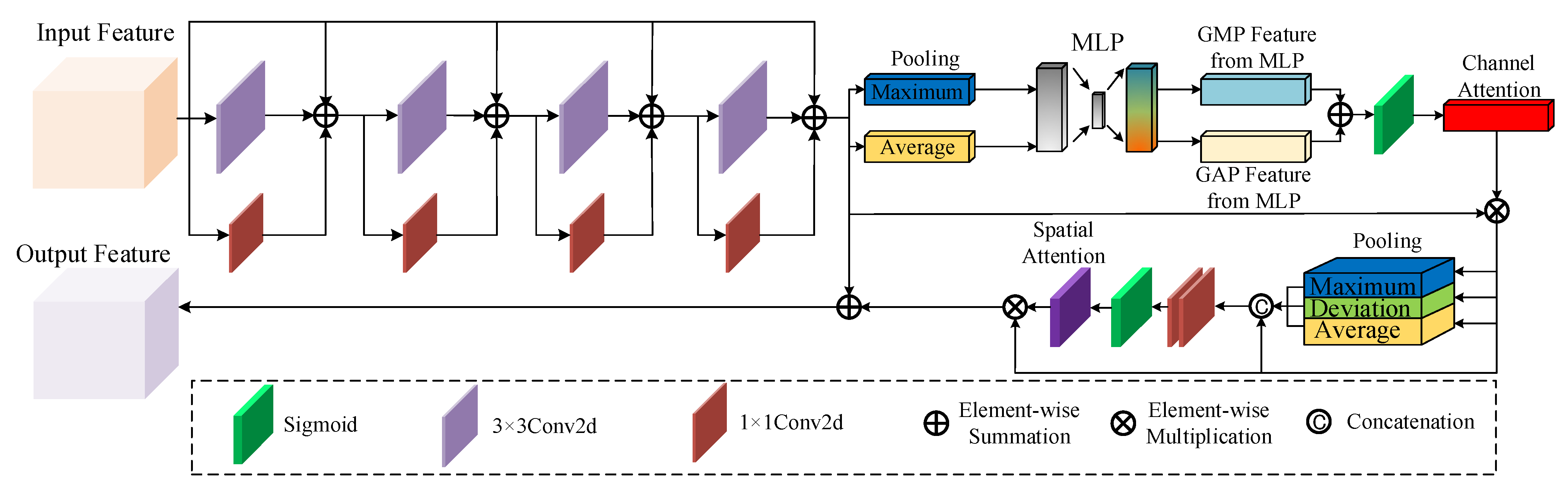
In 2017, Badrinarayanan et al. [10] proposed the Convolutional Block Attention Module (CBAM). CBAM combines the Channel Attention Module (CAM) and Spatial Attention Module (SAM) in a cascaded manner. As for CAM, Global Average Pooling (GAP) and Global Max Pooling (GMP) are firstly used to compress the spatial dimensions of the input features and condense spatial information [32]. Then, the correlation between channels is modeled through a Multilayer Perceptron (MLP) and the Sigmoid activation function. The outputs from MLP are combined to obtain channel attention weight . Channel attention highlights dependencies between channels and enhances specific semantic feature representations. Similar to CAM, SAM uses global average pooling and global max pooling to compress the channel dimension of the input features and condense channel information. Spatial attention weight is generated through convolutions and activation functions. Spatial attention focuses on long-range spatial dependencies, thus reducing the limited receptive field problem. The computation process of CBAM is shown in Equation (1), where represents input feature map, represents output feature map, and denotes element-wise multiplication between matrices.
Li et al. [32] constructed the SC-U2-Net network for sea ice segmentation. They added a multilayer CBAM into multiple locations of the network in order to extract more useful spatial and channel information, pay more attention to local features, and improve the generalization performance. Li et al. [34] proposed a novel algorithm, AttentionFGAN, for infrared and visible image fusion. They introduced a multiscale attention mechanism into the generator and two discriminators. In their network, the discriminators are constrained to pay more attention to the target information rather than all the information. The experiment results showed that the attention mechanism can effectively improve the target feature extraction capability. Additionally, the algorithm is superior to other algorithms in various scenarios.
3. Methodology
3.1. Overview
In this manuscript, a method for extracting photovoltaic panels from high-resolution optical remote sensing images guided by prior knowledge (PKGPVN) is proposed, as shown in Figure 1.
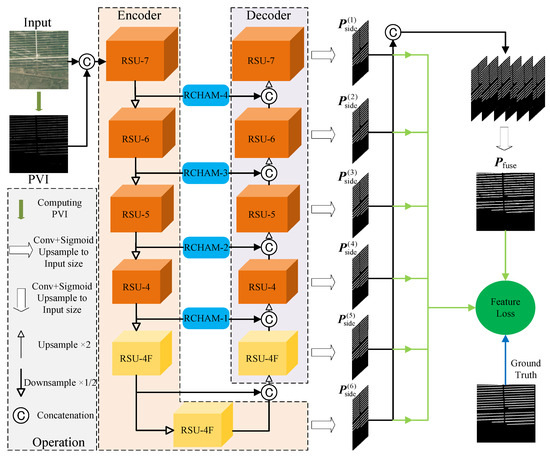
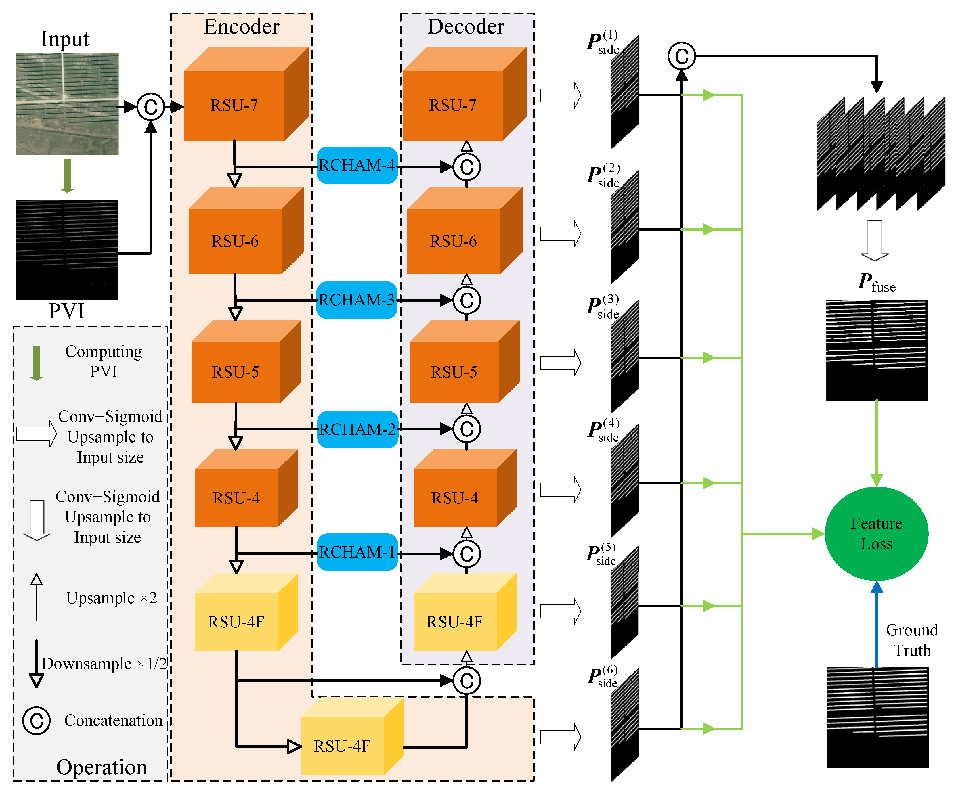
Figure 1.
The architecture of PKGPVN. PVI denotes the Photovoltaic Index; it is generated by the input image. RSU denotes the Residual U-block. RCHAM denotes the Residual Convolution Hybrid Attention Module. denotes the sub-prediction maps from the decoder and the last encoder. denotes the final prediction map; it is generated by the concatenated . Feature Loss is one of the loss functions in this paper.
Firstly, a Photovoltaic Index (PVI) is constructed and concatenated with the PV panel image, and they are sent to the network. The network uses RSU to form a U-shaped encoder–decoder structure. On this basis, residual structures, multilayer convolution, and attention mechanisms are introduced into the skip-connection part, forming a Residual Convolution Hybrid Attention Module (RCHAM). This module is used to reduce the semantic differences between shallow features and deep features, improve the capability of extracting effective features, and reduce the loss of local and global contextual information. Then, sub-prediction maps are generated from the decoder and the last encoder by using a 3 × 3 convolutional kernel and Sigmoid activation function. These sub-prediction maps are upsampled to match the size of the input. The concatenated sub-prediction maps are passed through a 1 × 1 convolutional kernel and Sigmoid activation function to generate the final prediction map . Finally, a multiscale Feature Loss (FL) function is designed, which calculates the L2 norm between the prediction map and the ground truth at the feature level to supervise the results. To illustrate the PKGPVN in detail, we provide pseudocode of it in Appendix A.
Section 3 introduces the design of the Photovoltaic Index, Residual Convolution Hybrid Attention Module, and Feature Loss function in our network.
3.2. Photovoltaic Index
According to a previous study [35], it has been proven that adding any bands that are linearly independent of the original image can always improve the performance of the constrained energy minimization operator in multispectral or hyperspectral remote sensing object detection. Chen et al. [6] confirmed the effectiveness of combining normalized indices (such as Normalized Difference Vegetation Index (NDVI), Normalized Difference Water Index (NDWI), and Normalized Difference Built-up Index (NDBI)) with multispectral images (Landsat8 OLI) for identifying large-scale PV plants. As presented in Section 2.1, Wang et al. [19] combined the Visible Difference Vegetation Index (VDVI) with RGB images to improve the separability of buildings from green areas. Based on these studies, an additional band with the ability to differentiate between objects and backgrounds was added to the optical remote sensing image in our method. By incorporating this approach, the confusion between PV panels and non-PV panels, frequently encountered during the extraction process by many models, can be significantly reduced.
Regarding the PV panel extraction task, there are some studies based on optical remote sensing images in red, green, and blue bands. In 2023, Yan et al. [36] proposed a benchmark dataset, AIR-PV, and evaluated some baseline methods on it. Wang et al. [17] trained their semantic segmentation model with the PVP dataset in the same year. Both studies demonstrated that accurate PV panels area can be extracted using red, green, and blue band images. Therefore, we used RGB band information to extract PV panel information.
The core part of crystalline silicon photovoltaic modules is the solar cell, which mostly appears in a deep blue color to enhance the absorption of sunlight [37]. In order to further determine the optical differences between different bands of PV panels, we randomly selected 100 images from the AIR-PV dataset [36] and statistically analyzed the pixel values of the PV panels and non-PV panels (such as roads, substations, and vegetation) in each band. As shown in Figure 2, it can be observed that the prominent feature of the PV panels compared to other objects is the significant difference between the pixel mean values of the blue band and the red band. The pixel values of the blue, green, and red bands decrease sequentially. In addition, previous studies have shown that the spectral curve of PV panels exhibits a reflection peak in the blue band and an absorption valley in the red band [38], which is consistent with the statistical results of this paper.
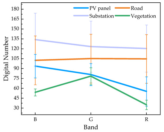
Figure 2.
Optical characteristics of different objects (mean ± standard deviation). These objects include photovoltaic panel, road, substation, and vegetation.
In order to effectively improve the performance of PV panel extraction, the added bands cannot be linear combinations of the original image bands [39]. Therefore, based on the optical and reflective characteristics of PV panels in the blue and red bands, we constructed the Photovoltaic Index (PVI), as shown below, to serve as prior knowledge, and added it to the original image to differentiate between PV panels and non-PV panels.
In Equation (2), denotes the red band, denotes the green band, and denotes the blue band. After obtaining the PVI, it is concatenated with the original image. They serve as the input to the first encoder in the network together in order to suppress background noise and reduce issues of missing extractions and background misjudgments.
3.3. Residual Convolution Hybrid Attention Module
In the U-Net and U2-Net, the output of each stage in the encoding process is copied to the corresponding stage in the decoding process, known as skip-connection. Skip-connection can compensate for the loss of low-level feature information caused by downsampling during the encoding process. However, using conventional skip-connection alone can easily lead to spatial information loss, and redundant information on feature channels can be easily retained. Additionally, the features from the encoder and corresponding decoder in the skip-connection often have significant semantic differences [40].
On this basis, aiming to reduce the aforementioned practical issues and further improve the accuracy and completeness of the PV panel extraction, we propose the Residual Convolution Hybrid Attention Module (RCHAM) to replace the conventional skip-connection, as shown in Figure 3. Based on the residual structure, the features derived from the encoder are subjected to 1 × 1 and 3 × 3 convolutional kernels to reduce semantic differences at first. As the hierarchical levels of the encoding and decoding structures deepen, the semantic differences between the encoder features and corresponding decoder features diminish. Therefore, a non-fixed number of convolutional kernel layers are designed in the RCHAM-i (i = 1, 2, 3, 4). We use a combination of i-layer 1 × 1 and 3 × 3 convolutional kernels in parallel. After the aforementioned nonlinear convolution operations, the channel and spatial attention weights are computed to emphasize and optimize features. These weights allow the network to focus on important information and ignore irrelevant information. Through a series of convolution and attention mechanisms, our method can introduce more semantic information into shallow features, enabling each level of output features to concentrate on effective information. Thus, the RCHAM can improve the ability of the model to extract PV panels features and achieve the integration of shallow and high-level semantic features. Furthermore, since the RCHAM is based on a residual structure, the proposed method enhances the network’s fitting capability and ensures the non-negativity of the accuracy improvement after adding the RCHAM.

Figure 3.
The architecture of the Residual Convolution Hybrid Attention Module (RCHAM-4). The input feature is processed by 1 × 1 and 3 × 3 convolutional kernels in parallel, and then the optimized feature is processed by the attention mechanism in series to obtain the output feature.
3.4. Feature Loss
After the above processing, the network is capable of extracting intra-level and inter-level information from images of different sizes, preserving valuable features and reducing object misjudgments caused by the complex backgrounds. However, in remote sensing images, the sample categories of PV panels are uneven, and edge information is easily influenced by noise. Therefore, preserving edge information becomes one of the most important aspects in extracting PV panels. In order to mitigate the loss of edge and detail information, we designed a loss function as shown in Equation (3).
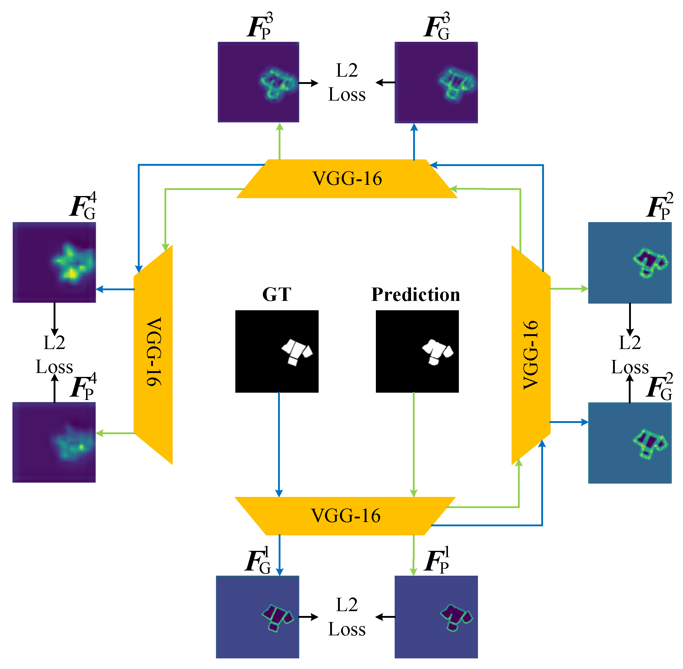
where is the total loss in our network. is the Binary Cross-Entropy (BCE) loss, which has been widely used and proven in various visual tasks [31,41]. is the Feature Loss (FL), which aims to optimize the edges and details of the extraction results at the feature level [42]. Specifically, we draw on the ideas of loss function from [43]. We used a pretrained classifier, VGG-16 from PyTorch, to extract the multiscale features of the predicted map and the ground truth (GT), and calculated the L2 norm between the features for pixel-to-pixel matching. The definition of is as follows:
As shown in Figure 1, there are six sub-prediction maps and they come from five decoders and the last encoder. In Equation (4), it is necessary to compute the loss between each sub-prediction map and the GT. Therefore, was set to 6. is the loss of the sub-prediction maps ; it aims to fully exploit the inherent contextual information among multiple sub-prediction maps. refers to the , , , , , and in Figure 1. is the loss of the final prediction map . and denote the weights of each loss term.
In Equation (6), represents the i-th layer feature extracted from the prediction values, represents the i-th layer feature extracted from the GT, and represents the L2 norm calculation between the i-th layer features.
The architecture of the FL is visually depicted in Figure 4. Within this framework, lower-level feature maps contain edge and detail information, while higher-level feature maps contain positional information. The FL can supervise the prediction results at different scales of feature levels, address complex boundary challenges, and preserve the contours and structures of PV panels as comprehensively as possible.
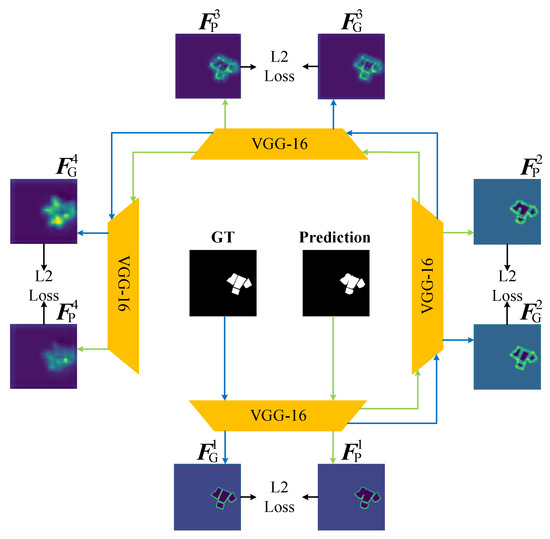
Figure 4.
Feature Loss (FL) structure diagram. denotes the i-th layer feature extracted from the prediction. denotes the i-th layer feature extracted from the ground truth (GT). The FL can supervise the prediction at four scales of features.
4. Results
This section introduces the validation of the results. Section 4.1 presents two publicly available datasets, AIR-PV and PVP, and the parameter settings in the experiments. Section 4.2 introduces four metrics to evaluate the methods objectively. Section 4.3 includes qualitative and quantitative experiments of PKGPVN and comparison methods.
4.1. Datasets and Parameter Settings
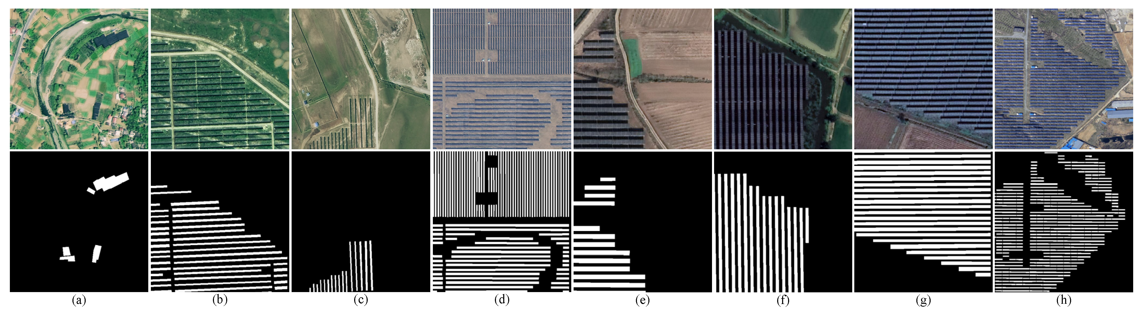
AIR-PV dataset [36]: This publicly available dataset is from the Gaofen-2 satellite. For the Gaofen-2 satellite, the spatial resolution of the panchromatic band and the multispectral bands is 0.8 m and 3.2 m, respectively. After image fusion, the AIR-PV dataset based on visible light in the red (0.63~0.69 μm), green (0.52~0.59 μm), and blue (0.45~0.52 μm) bands was constructed. It includes 0.8 m/pixel imagery with a pixel resolution of 512 × 512. The total number of images in this dataset is 5000 and the format is PNG. Additionally, this dataset contains over 300,000 PV panels distributed in five western provinces of China (Inner Mongolia, Qinghai, Gansu, Shanxi, and Yunnan). It provides diverse backgrounds of PV panels, including residential areas, grasslands, drylands, and desert, as shown in Figure 5a–d.
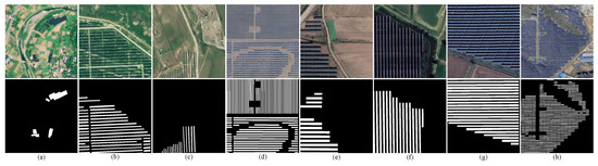
Figure 5.
AIR-PV and PVP datasets. The background of different ground objects: (a) residential areas; (b) grasslands; (c) drylands; (d) desert; (e) farmlands; (f) water; (g) grasslands; (h) drylands.
PVP dataset [17]: This dataset is from Google Earth, Tianditu, and Mapbox. Similarly, the fused image contains red, green, and blue bands. The spatial resolutions of Google Earth, Tianditu, and Mapbox are 0.54 m, 0.6 m, and 0.5 m, respectively. This dataset includes 4640 image tiles with 512 × 512 pixels in total, and the format is TIFF. Examples of the PVP dataset are illustrated in Figure 5e–h.
The experimental setup involves using the Windows 10 64-bit operating system, an Intel(R) Core(TM) i7-8550U CPU @ 1.80 GHz, and an NVIDIA GeForce RTX 3090 GPU with 24 GB memory. The software environment is Python 3.8 and PyTorch 1.11.0. The batch size is 4, and 100 iterations are used. The initial learning rate is 0.001, and the optimizer is the Stochastic Gradient Descent (SGD) optimizer. Since the final prediction map was generated from the sub-prediction map, both weights ( and ) in the Feature Loss were set to 1 as they are equally important. All samples were divided into training and testing datasets in a ratio of 7:3.
4.2. Evaluation Metrics
In order to evaluate the quality of the extraction results more accurately, we selected four evaluation metrics: Intersection-over-Union (IoU), Precision, Recall, and F1-score [44,45]. The calculation process is as follows:
where TP denotes the number of successfully detected objects, FP denotes the number of successfully detected backgrounds, FN denotes the number of objects that were missed [46], IoU reflects the degree of overlap between the prediction map and the ground truth, Precision reflects the model’s ability to distinguish negative samples, Recall reflects the model’s ability to identify positive samples, and F1-score reflects the model’s robustness. The larger the values of these four metrics, the higher the quality of the extraction results and the better the performance of model.
4.3. Comparative Experiments
In this study, the proposed PKGPVN was trained according to the parameter settings in Section 4.1. In order to compare performance, seven commonly used object detection models were trained under the same conditions. These models include U-Net [9], FCN [47], SegNet [10], D-LinkNet [48], BASNet [41], U2-Net [31], and SeaNet [49]. We conducted qualitative and quantitative experiments on the AIR-PV dataset and PVP dataset.
4.3.1. Experiments on the AIR-PV Dataset
Figure 6 shows the extraction results of PKGPVN and comparison methods on the AIR-PV dataset.
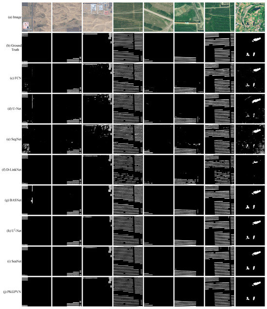
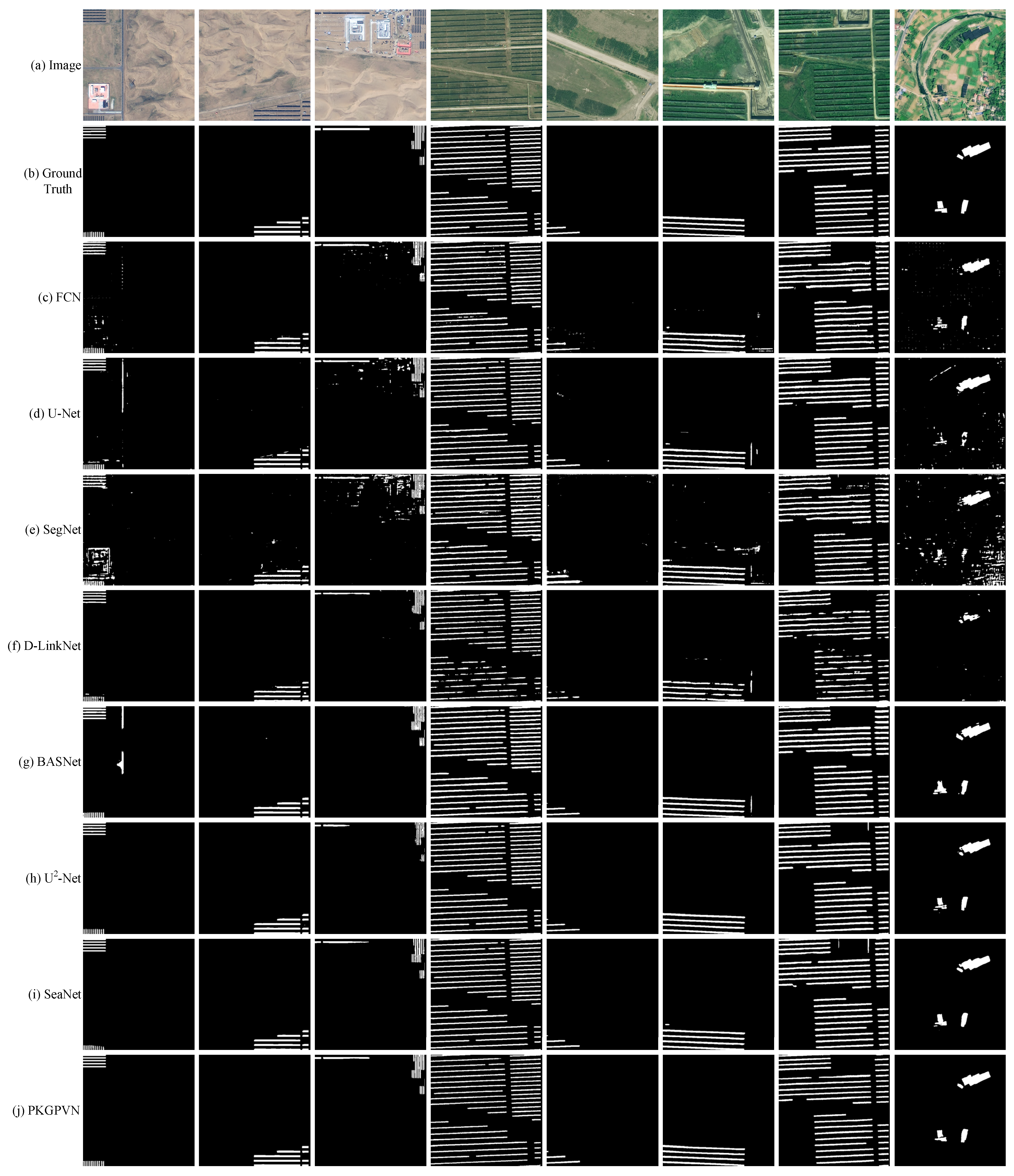
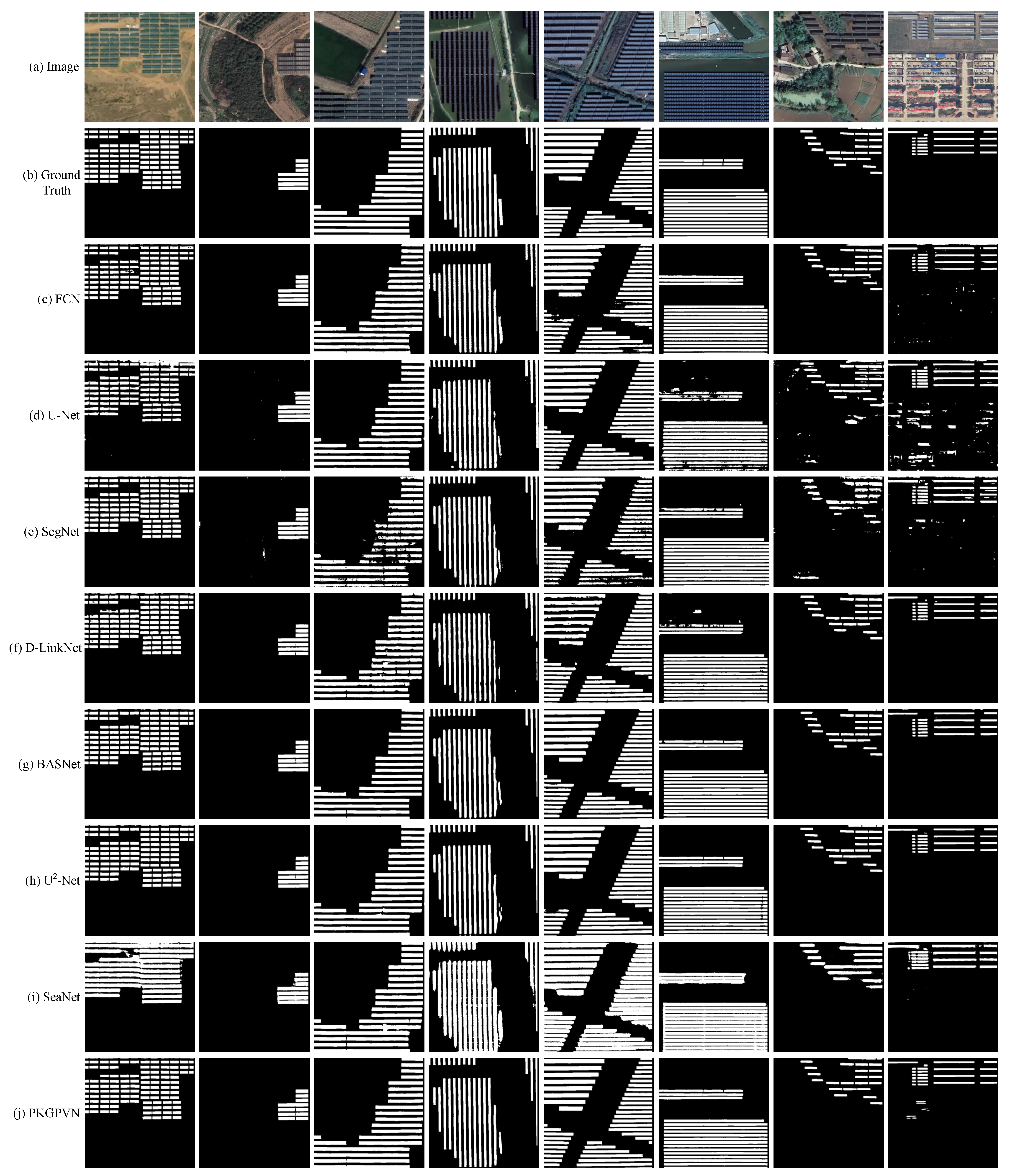
Figure 6.
Extraction results of PV panels using different methods on the AIR-PV dataset. The backgrounds in the first to third columns are desert, the backgrounds in the fourth column and the fifth column are drylands, the backgrounds in the sixth column and the seventh column are grasslands, the background in the eighth column is residential area.
The backgrounds in the first to third columns are desert. From the results, it can be observed that FCN, U-Net, and SegNet have certain errors. In the first column, U-Net and BASNet misclassify roads as PV panels. In the third column, D-LinkNet, BASNet, U2-Net, and SeaNet have lower completeness and fail to detect all PV panels. In contrast, PKGPVN significantly reduces the omission and misclassification when facing objects that are easily confused with PV panels. This confirms that the addition of the PVI and RCHAM to the network can address the problem of misjudgment and enhance the completeness of PV panel extraction.
The backgrounds in the fourth column and the fifth column are drylands, where there is significant contrast between the PV panels and the background. The results show that PKGPVN effectively controls the smoothness of the boundaries. This confirms that the inclusion of FL allows the network to process edges more completely and smoothly.
The backgrounds in the sixth column and the seventh column are grasslands, where there is a small difference between the PV panels and the background, making them easily confused. All the comparison methods tend to misclassify shadows as PV panels, while PKGPVN generates the most accurate results.
The background in the eighth column is residential area, which significantly increases the difficulty of PV panel extraction due to the complexity and diversity of targets. The results show that FCN, U-Net, and SegNet have more misclassifications; D-LinkNet fails to detect all the PV panels; and BASNet, U2-Net, and SeaNet present the hollow phenomenon. In contrast, PKGPVN achieves better closure and clearer edges in the extraction results.
In conclusion, compared to other methods, our proposed method reduces the issues of missed extractions and background misjudgments. The results have more complete PV panels with smoother edges and significant visual improvement.
In order to comprehensively evaluate the feasibility and accuracy of the models, quantitative experiments were conducted as detailed in this section. We used IoU, Precision, Recall, and F1-score to analyze the extraction results of our PKGPVN and comparison methods. The results of the experiments on the AIR-PV dataset are shown in Table 2.
Table 2.
Performance comparison table of different methods on the AIR-PV dataset (unit: %).
Table 2 indicates that the visual results in Figure 6 are consistent with the evaluation metrics, and our PKGPVN is overall superior to most of the other comparison methods. The highest accuracy values are achieved in terms of IoU, Precision and F1-score, which are 82.34%, 91.41%, and 90.25% respectively. The higher value of IoU suggests that RCHAM enhances the completeness of the PV panel extraction, resulting in better alignment between the extracted PV panels and the ground truth, as shown in the second column and the fourth column of Figure 6. The higher value of Precision indicates a lower number of false positives, meaning that fewer instances of other categories are incorrectly predicted as positive. It confirms the favorable effect of PVI in addressing misclassifications, as demonstrated in the sixth column of Figure 6. The higher F1-score value suggests that RCHAM and Feature Loss effectively balance Precision and Recall, resulting in a more complete and accurate extraction of PV panel regions and boundaries, as observed in the fifth column and the eighth column of Figure 6. Compared to BASNet, the value of Recall decreased by 0.53%, which can be attributed to the fact that BASNet tends to over-detect, leading to a higher Recall value, as evident in the first column and the sixth column of Figure 6.
Compared to the baseline U2-Net, there is an improvement of 3.22%, 0.40%, 3.28%, and 2.29% in terms of IoU, Precision, Recall, and F1-score, respectively, which demonstrates the feasibility and effectiveness of PVI, RCHAM, and FL.
Qualitative and quantitative experiments demonstrate that our proposed PKGPVN can extract PV panels in different scenarios, suppress background pixel noise, and reduce missed extractions and background misjudgments. Additionally, it aims to preserve boundary information and effectively prevent the loss of fine details.
4.3.2. Experiments on the PVP Dataset
Figure 7 shows the extraction results of PKGPVN and other comparison methods on the PVP dataset. It is worth noting that the extracted PV panels of our method are closely aligned with the GT, with very minimal errors. In regions with complex backgrounds, the PV panels extracted by other methods may exhibit omission or false detection, while our PKGPVN maintains the integrity and edge clarity of the PV panels. For example, in the last column of Figure 7, structures like houses and shadows are easily confused with PV panels. FCN, U-Net, and SegNet exhibit more misclassification, while D-LinkNet, BASNet, U2-Net, and SeaNet show lower completeness and fail to detect all the PV panels. The results obtained by our PKGPVN not only match the GT but also detect the PV panels missed in the GT, which further validates the superiority of our method in the PV panel extraction task, as shown in Figure 8.
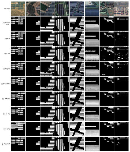
Figure 7.
Extraction results of PV panels using different methods on the PVP dataset.
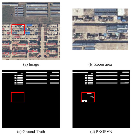
Figure 8.
Detailed presentation of the last column of Figure 7. (a) Source image; (b) enlarged red rectangular box area in source image; (c) unlabeled PV panels in GT; (d) detected PV panels in our PKGPVN.
Table 3 shows the quantitative results of our PKGPVN compared with other methods on the PVP dataset. PKGPVN achieves IoU, Precision, and F1-score values of 91.71%, 96.51%, and 95.74%, respectively, which are better than other methods. Compared to SeaNet, the value of Recall decreased by 4.41%. SeaNet guarantees the completeness of the results but exhibits over-extraction, as evident in the first column and the third column of Figure 7. Compared to the baseline U2-Net, there is an improvement of 1.03%, 1.11%, 0.41%, and 0.85% in terms of IoU, Precision, Recall, and F1-score, respectively, which shows that our PKGPVN is feasible and robust in different datasets.
Table 3.
Performance comparison table of different methods on the PVP dataset (unit: %).
Qualitative and quantitative experiments demonstrate that our PKGPVN can extract complete PV panels in different datasets and reduce missed extractions and background misjudgments. The results show that the PV panels are more complete, the edge is smoother, and the visual effect is remarkable.
5. Discussion
To further verify the effectiveness of PVI, RCHAM, and FL on PV panel extraction, three ablation experiments are conducted as detailed in this section. Additionally, Section 5.1 presents a generalization experiment of PVI to verify its feasibility on other datasets.
5.1. The Effectiveness of PVI
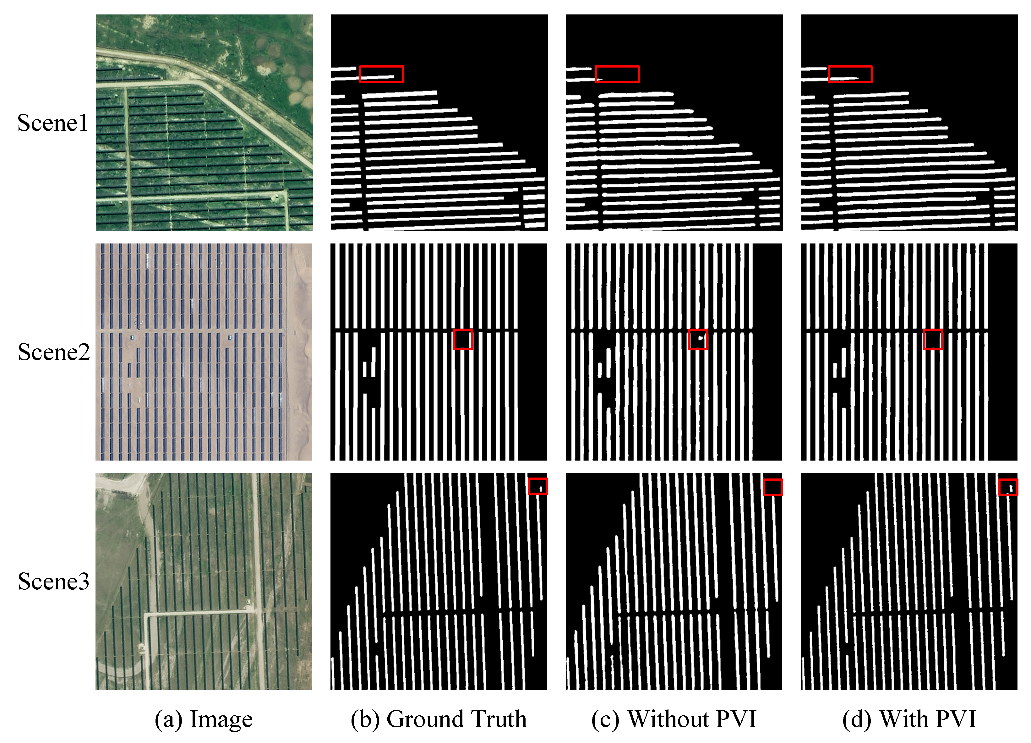
The role of PVI is to suppress background noise and reduce panel omissions and background misclassifications. In this section, a comparison is made between a network without PVI and a network with PVI, while keeping other experimental settings unchanged. Figure 9 shows the extraction results with and without PVI, from left to right: the original image, the ground truth, the result without PVI, and the result with PVI. Figure 9 indicates that there are some instances of omissions when dealing with small objects without PVI, although most of the PV panels can be extracted, as seen in scene 1 and scene 3. The network without PVI is more prone to confusing PV panels with non-targets such as substations in scene 2.
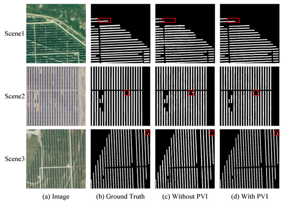
Figure 9.
Visualization results of PVI ablation experiment. The red rectangles indicate differences.
Table 4 presents the metric values before and after adding PVI for the three scenes in Figure 9. From Table 4, it can be observed that the network with PVI has certain advantages in terms of IoU, Precision, and F1-score. It is worth noting that Recall decreased by 1.15% and 5.91% in scene 2 and scene 3, respectively (indicated in bold and italic). The network without PVI tends to mistakenly extract non-PV panels as PV panels, resulting in an “inflated” Recall value but a lower Precision value. The results of PVI ablation experiments further illustrate the necessity of adding PVI, and validate that PVI increases the model’s ability to distinguish between objects and backgrounds, improving the accuracy of the PV panel extraction.
Table 4.
Accuracy evaluation of PVI ablation experiment. The last row indicates the rise in metric values (unit: %).
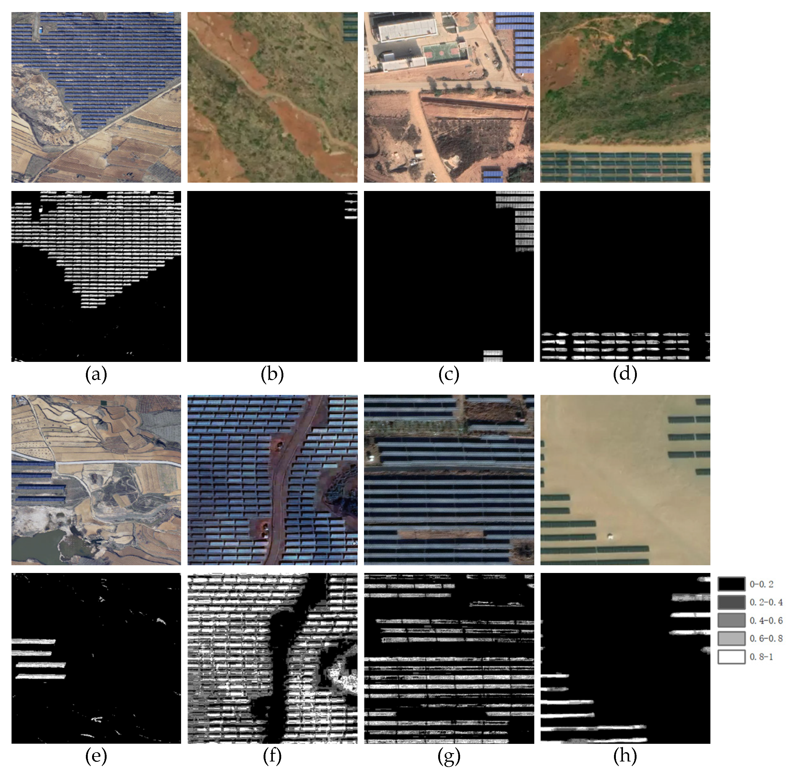
To verify the effectiveness of PVI on other datasets, we designed a generalization experiment for PVI. As described in Section 3.2, we used the pixel value differences between the blue and red bands to highlight PV panels on the AIR-PV dataset when designing the PVI. Therefore, for this experiment, the dataset was selected from the PVP dataset provided in PVNet [17]. Figure 10 shows the visualization results for eight images. The results show that the majority of the PV panel areas can be extracted using PVI. Figure 10a–d show significant contrast between the PV panels and background, and PVI values are all above 0.6. However, there are still some background misjudgments due to the similarity of the pixel values between the PV panels and other objects, as seen in Figure 10e,f. In order to evaluate the PV panel extraction ability of PVI more objectively and clearly, first, we calculated the PVI of all the images in the PVP dataset. Then, we transformed the PVI images into binary images using the Otsu [50] method. The evaluation metrics show that the mean values of IoU and F1 are 57.64% and 68.49%. They indicate that PVI can basically extract the PV panels and serve as prior knowledge to improve the accuracy of the model. Thus, the above experiments demonstrate the generalization capability of PVI on other datasets.
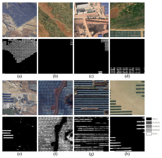
Figure 10.
Visualization results of PVI generalization experiment. (a) Concentrated PV panels in terraced fields; (b) discrete PV panels in grasslands; (c) discrete PV panels in residential areas; (d) concentrated PV panels in grasslands; (e) discrete PV panels in terraced fields; (f) concentrated PV panels in drylands; (g) concentrated PV panels in farmlands; (h) discrete PV panels in desert. Each group includes the PV panel images above and the PVI visualization results below.
5.2. The Effectiveness of RCHAM
The role of RCHAM is to strengthen the interaction between shallow features and deep features, increase the extraction capability of effective features, and improve the completeness of PV panel regions. Figure 11 shows that using the network without RCHAM led to irregular contours of extraction results in scene 6 and also led to a disconnection between the PV panels in scene 5. The network with RCHAM can accurately separate adjacent PV panels in dense regions with good noise immunity while preserving local and global contextual information.
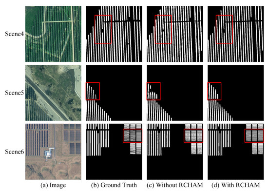
Figure 11.
Visualization results of RCHAM ablation experiment. The red rectangles indicate difference.
Table 5 presents the metric values before and after adding RCHAM for the three scenes in Figure 11. In the field of image processing, both local and global contextual information are crucial factors for accuracy [51]. From Table 5, it can be seen that adding RCHAM improves the performance of the network. Similar to the results of the PVI ablation experiments, Recall decreased by 7.47% and 1.94% in scene 4 and scene 6, respectively, which aligns with the visual effects in Figure 11. The results of the RCHAM ablation experiments further validate that RCHAM reduces the issues of incomplete regions and mismatched boundaries, improves the accuracy of the PV panel extraction, and preserves rich contextual information.
Table 5.
Accuracy evaluation of RCHAM ablation experiment. The last row indicates the rise in metric values (unit: %).
5.3. The Effectiveness of FL
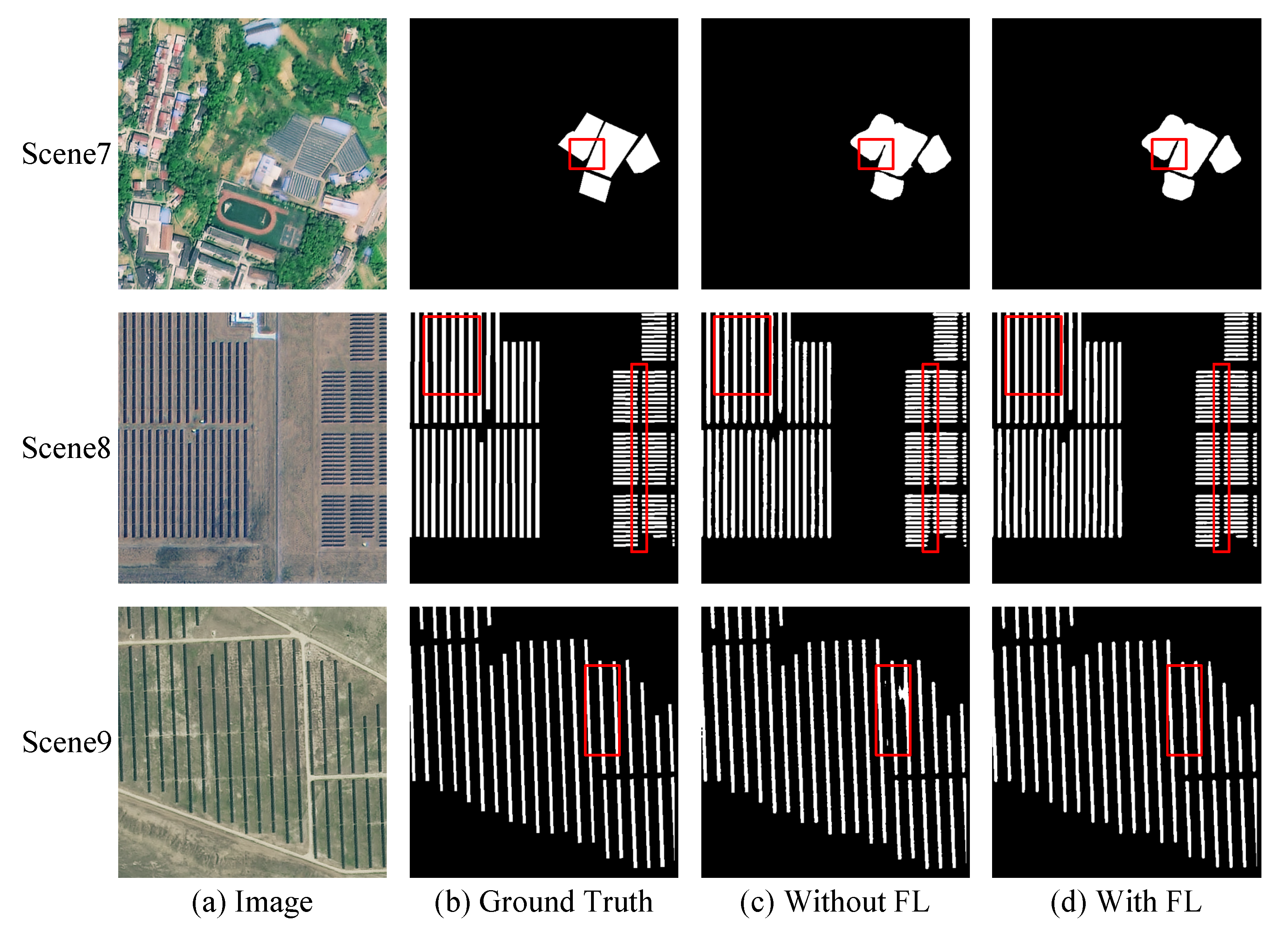
The role of Feature Loss is to reduce the phenomenon of blurred edges and preserve more boundary information. Figure 12 shows that the network without FL led to blurred edges in scene 8 and scene 9 and adjacent panels sticking in scenes 7 and 8. The network with FL improves the smoothness of the PV panels’ edges and better preserves the details.
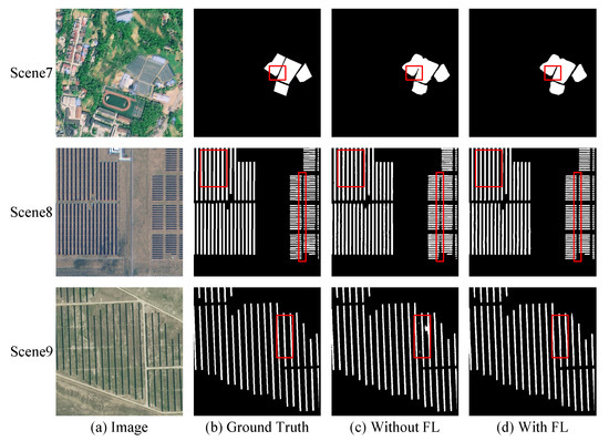
Figure 12.
Visualization results of FL ablation experiment. The red rectangles indicate differences.
Table 6 presents the metric values before and after adding FL for the three scenes depicted in Figure 12. From Table 6, it can be seen that adding FL improves the performance of network slightly. However, Recall decreased by 0.66% and 1.15% in scenes 7 and 8, respectively, due to the impact of FL in optimizing the boundaries. In the absence of FL, the sticking and blurring of edges between the PV panels led to the misclassification of boundary pixels, resulting in “inflated” Recall values. The results of the FL ablation experiment further validate that FL promotes the network to focus on fine details and low-level features such as edges, making the extracted boundary more precise and improving the accuracy in the PV panel extraction.
Table 6.
Accuracy evaluation of FL ablation experiment. The last row indicates the rise in metric values. (unit: %).
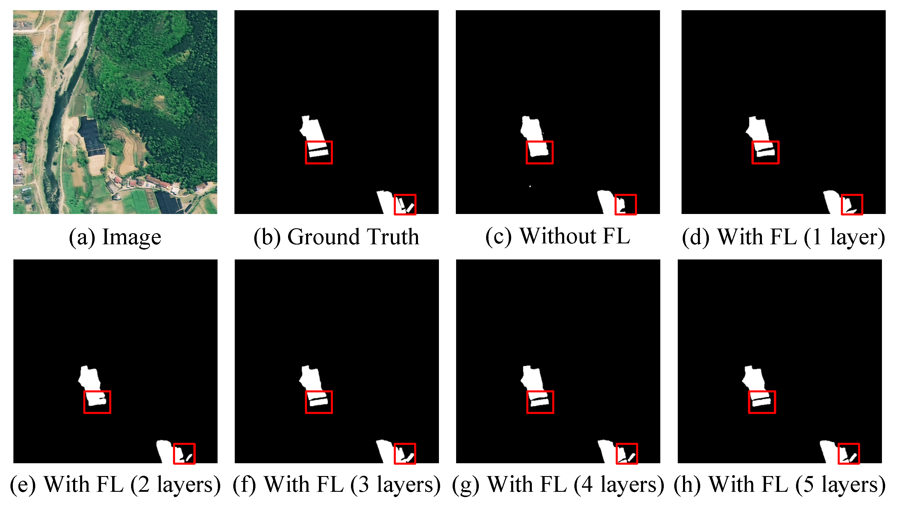
In this manuscript, there are four layers of FL. To avoid redundancy, we designed an ablation experiment to determine the number of FL layers. Figure 13c shows the result without FL; Figure 13d–h show the results with one, two, three, four, and five layers of FL, respectively. Evidently, the results with FL have clearer and more accurate boundary information. However, the results show little visual difference when the number of FL layers increases from three to five (Figure 13f–h). Table 7 presents the metric values for different numbers of FL layers, shown in Figure 13. From Table 7, it can be seen that the IoU, Precision, Recall, and F1-score values are 90.19%, 95.33%, 94.36%, and 94.84% in FL (four layers). They are all higher than the values for other numbers of FL layers. In particular, the Recall of FL (five layers) is the same as that of FL (four layers), while the other three metrics are lower than those of FL (four layers). The metrics on all the testing dataset images similarly corroborate the superiority of FL (four layers), as seen in Table 8. Therefore, FL (four layers) is superior to the others, both in terms of visual effects and numerical metrics.

Figure 13.
FL layers ablation experiment. The red rectangles indicate differences. (c) The result without FL. (d–h) The results with one, two, three, four, and five layers of FL, respectively.
Table 7.
Accuracy evaluation of FL layers ablation experiment in Figure 13 (unit: %).
Table 8.
Accuracy evaluation of FL layers ablation experiment in testing datasets (unit: %).
6. Conclusions
From the perspective of social development and energy utilization, extracting PV panels from high-resolution optical remote sensing images is a research task of great significance. In this study, we constructed a PVI to serve as prior knowledge to reduce the confusion between PV panels and non-PV panels. In the encoder–decoder structure, RCHAM was designed to replace the conventional skip-connection. It reduces semantic differences among features from different levels, preserves effective feature information in both spatial and channel domains, and improves the completeness of the PV panel results. Additionally, was is integrated into the loss function to minimize the occurrence of blurred edges and preserve edge details as much as possible. Qualitative and quantitative experiments demonstrate that the proposed PKGPVN outperforms other comparison methods in terms of visual effects and evaluation metrics. The effectiveness of our PKGPVN was further validated through three ablation experiments. The experiments indicate that our PKGPVN has certain advantages in reducing the problems of missed extractions and background misjudgments, ensuring the completeness of extraction, and keeping boundaries smooth, with strong robustness.
However, there is still space for further improvement. While we adopted the AIR-PV dataset, which contains four different backgrounds, the extraction effect for the PV panels in other regions needs verification using diverse datasets. Future work will involve optimizing the model and enhancing the model’s generalizability and practicality by employing different datasets. Furthermore, applying PV panel extraction results to power generation estimation is a major challenge. We will predict the power generation of solar systems based on deep learning methods by combining meteorological data and geographical coordinate information.
Author Contributions
Conceptualization, W.L. and H.H.; methodology, W.L. and L.J.; software, W.L. and X.L.; validation, W.L., H.H. and L.J.; formal analysis, H.H. and Y.Z.; investigation, L.J., Y.Z. and W.L.; writing—original draft preparation, W.L. and J.L.; writing—review and editing, L.J., Y.Z., J.L. and X.L.; visualization, W.L.; supervision, H.H.; project administration, H.H.; funding acquisition, H.H. All authors have read and agreed to the published version of the manuscript.
Funding
This research was funded by the National Key Research and Development Program of China, grant number 31400.
Data Availability Statement
The data used for training and testing set are available at: https://github.com/AICyberTeam/AIR-PV-dataset and https://github.com/RS-Wangjx/PVP-Dataset, accessed on 27 November 2023.
Conflicts of Interest
The authors declare no conflict of interest.
Abbreviations
Here are the abbreviations covered in this manuscript:
| PV | Photovoltaic |
| PVI | Photovoltaic Index |
| RCHAM | Residual Convolution Hybrid Attention Module |
| FL | Feature Loss |
| UAV | Unmanned Aerial Vehicle |
| CNN | Convolutional Neural Network |
| SVM | Support Vector Machine |
| RF | Randon Forest |
| RSU | Residual U-block |
| CBAM | Convolutional Block Attention Module |
| CAM | Channel Attention Module |
| SAM | Spatial Attention Module |
| MLP | Multilayer Perceptron |
| BCE | Binary Cross-Entropy |
| GT | Ground Truth |
| IoU | Intersection-over-Union |
Appendix A
| Algorithm A1. PV panel extraction method (PKGPVN). |
| Input: : PV panels images with shape [b, c, h, w] |
| Output: : final prediction map |
| 1: Compute using Equation (2): |
| B = [ : , 0:1, : , : ], G = [ : , 1:2, : , : ], R = [ : , 2:3, : , : ] |
| = (B − R)/(R + G + B) |
| 2: Get network input: |
| = torch.cat([, ], 1) |
| 3: while epoch 100 do |
| 4: Get encoder output: |
| = RSU () |
| 5: Get RCHAM output: |
| = RCHAM () |
| 6: Get decoder output: |
| = RSU (torch.cat(], dim = 1)) |
| 7: : |
| = F.interpolate(, size = [h, w], mode = ‘bilinear’, align_corners = False) |
| 8: : |
| = nn.Conv2d(torch.cat([], dim = 1)) |
| 9: using Equations (3)–(6) |
| 10: |
| 11: end while |
| 12: Obtain the PV panel extraction results through step 4 to 8 |
References
- Hou, J.; Luo, S.; Cao, M. A Review on China’s Current Situation and Prospects of Poverty Alleviation with Photovoltaic Power Generation. J. Renew. Sustain. Energy 2019, 11, 013503. [Google Scholar] [CrossRef]
- Tian, J.; Ooka, R.; Lee, D. Multi-scale solar radiation and photovoltaic power forecasting with machine learning algorithms in urban environment: A state-of-the-art review. J. Clean. Prod. 2023, 426, 139040. [Google Scholar] [CrossRef]
- Yao, Y.; Hu, Y. Recognition and Location of Solar Panels Based on Machine Vision. In Proceedings of the 2017 2nd Asia-Pacific Conference on Intelligent Robot System (ACIRS), Wuhan, China, 16–18 June 2017; pp. 7–12. [Google Scholar] [CrossRef]
- Malof, J.; Hou, R.; Collins, L.; Bradbury, K.; Newell, R. Automatic Solar Photovoltaic Panel Detection in Satellite Imagery. In Proceedings of the 2015 International Conference on Renewable Energy Research and Applications (ICRERA), Palermo, Italy, 22–25 November 2015; pp. 1428–1431. [Google Scholar] [CrossRef]
- Malof, J.; Bradbury, K.; Collins, L.; Newell, R. Automatic Detection of Solar Photovoltaic Arrays in High Resolution Aerial Imagery. Appl. Energy 2016, 183, 229–240. [Google Scholar] [CrossRef]
- Chen, Z.; Kang, Y.; Sun, Z.; Wu, F.; Zhang, Q. Extraction of Photovoltaic Plants Using Machine Learning Methods: A Case Study of the Pilot Energy City of Golmud, China. Remote Sens. 2022, 14, 2697. [Google Scholar] [CrossRef]
- Zhang, R.; Newsam, S.; Shao, Z.; Huang, X.; Wang, J.; Li, D. Multi-scale adversarial network for vehicle detection in UAV imagery. ISPRS J. Photogramm. Remote Sens. 2021, 180, 283–295. [Google Scholar] [CrossRef]
- Li, J.; Yang, B.; Bai, L.; Dou, H.; Li, C.; Ma, L. TFIV: Multi-grained Token Fusion for Infrared and Visible Image via Transformer. IEEE Trans. Instrum. Meas. 2023, 72, 2526414. [Google Scholar] [CrossRef]
- Ronneberger, O.; Fischer, P.; Brox, T. U-Net: Convolutional Networks for Biomedical Image Segmentation. arXiv 2015, arXiv:1505.04597. [Google Scholar] [CrossRef]
- Badrinarayanan, V.; Kendall, A.; Cipolla, R. SegNet: A Deep Convolutional Encoder-Decoder Architecture for Image Segmentation. IEEE Trans. Pattern Anal. Mach. Intell. 2017, 39, 2481–2495. [Google Scholar] [CrossRef]
- Ji, S.; Wei, S.; Lu, M. Fully Convolutional Networks for Multisource Building Extraction from an Open Aerial and Satellite Imagery Data Set. IEEE Trans. Geosci. Remote Sens. 2018, 57, 574–586. [Google Scholar] [CrossRef]
- Mei, J.; Li, R.; Gao, W.; Cheng, M. CoANet: Connectivity Attention Network for Road Extraction from Satellite Imagery. IEEE Trans. Image Process. 2021, 30, 8540–8552. [Google Scholar] [CrossRef]
- Yu, J.; Wang, Z.; Majumdar, A.; Rajagopal, R. DeepSolar: A Machine Learning Framework to Efficiently Construct a Solar Deployment Database in the United States. Joule 2018, 2, 2605–2617. [Google Scholar] [CrossRef]
- Parhar, P.; Sawasaki, R.; Todeschini, A.; Reed, C.; Vahabi, H.; Nusaputra, N.; Vergara, F. HyperionSolarNet: Solar Panel Detection from Aerial Images. arXiv 2022, arXiv:2201.02107. [Google Scholar] [CrossRef]
- Zhu, R.; Guo, D.; Wong, M.; Qian, Z.; Chen, M.; Yang, B.; Chen, B.; Zhang, H.; You, L.; Heo, J.; et al. Deep solar PV refiner: A detail-oriented deep learning network for refined segmentation of photovoltaic areas from satellite imagery. Int. J. Appl. Earth Obs. Geoinf. 2023, 116, 103134. [Google Scholar] [CrossRef]
- Kirillov, A.; Wu, Y.; He, K.; Girshick, R. PointRend: Image Segmentation as Rendering. In Proceedings of the 2020 IEEE/CVF Conference on Computer Vision and Pattern Recognition (CVPR), Seattle, WA, USA, 13–19 June 2020; pp. 9796–9805. [Google Scholar] [CrossRef]
- Wang, J.; Chen, X.; Jiang, W.; Hua, L.; Liu, J.; Sui, H. PVNet: A novel semantic segmentation model for extracting high-quality photovoltaic panels in large-scale systems from high-resolution remote sensing imagery. Int. J. Appl. Earth Obs. Geoinf. 2023, 119, 103309. [Google Scholar] [CrossRef]
- Ahn, H.K.; Park, N. Deep RNN-Based Photovoltaic Power Short-Term Forecast Using Power IoT Sensors. Energies 2021, 14, 436. [Google Scholar] [CrossRef]
- Wang, Y.; Li, S.; Teng, F.; Lin, Y.; Wang, M.; Cai, H. Improved Mask R-CNN for Rural Building Roof Type Recognition from UAV High-Resolution Images: A Case Study in Hunan Province, China. Remote Sens. 2022, 14, 265. [Google Scholar] [CrossRef]
- Kruitwagen, L.; Story, K.; Friedrich, J.; Byers, L.; Skillman, S.; Hepburn, C. A global inventory of photovoltaic solar energy generating units. Nature 2021, 598, 604–610. [Google Scholar] [CrossRef]
- Li, P.; Zhang, H.; Guo, Z.; Lyu, S.; Chen, J.; Li, W.; Song, X.; Shibasaki, R.; Yan, J. Understanding rooftop PV panel semantic segmentation of satellite and aerial images for better using machine learning. Adv. Appl. Energy 2021, 4, 100057. [Google Scholar] [CrossRef]
- Redmon, J.; Divvala, S.; Girshick, R.; Farhadi, A. You Only Look Once: Unified, Real-Time Object Detection. In Proceedings of the 2016 IEEE Conference on Computer Vision and Pattern Recognition (CVPR), Las Vegas, NV, USA, 27–30 June 2016; pp. 779–788. [Google Scholar] [CrossRef]
- Li, L.; Wang, Z.; Zhang, T. GBH-YOLOv5: Ghost Convolution with BottleneckCSP and Tiny Target Prediction Head Incorporating YOLOv5 for PV Panel Defect Detection. Electronics 2023, 12, 561. [Google Scholar] [CrossRef]
- Girshick, R.; Donahue, J.; Darrell, T.; Malik, J. Rich Feature Hierarchies for Accurate Object Detection and Semantic Segmentation. In Proceedings of the 2014 IEEE Conference on Computer Vision and Pattern Recognition (CVPR), Columbus, OH, USA, 23–28 June 2014; pp. 580–587. [Google Scholar] [CrossRef]
- Girshick, R. Fast R-CNN. In Proceedings of the 2015 IEEE International Conference on Computer Vision (ICCV), Santiago, Chile, 7–13 December 2015; pp. 1440–1448. [Google Scholar] [CrossRef]
- Ren, S.; He, K.; Girshick, R.; Sun, J. Faster R-CNN: Towards Real-Time Object Detection with Region Proposal Networks. IEEE Trans. Pattern Anal. Mach. Intell. 2017, 39, 1137–1149. [Google Scholar] [CrossRef]
- He, K.; Gkioxari, G.; Dollár, P.; Girshick, R. Mask R-CNN. IEEE Trans. Pattern Anal. Mach. Intell. 2020, 42, 386–397. [Google Scholar] [CrossRef] [PubMed]
- Chen, L.; Zhu, Y.; Papandreou, G.; Schroff, F.; Adam, H. Encoder-Decoder with Atrous Separable Convolution for Semantic Image Segmentation. In Proceedings of the European Conference on Computer Vision (ECCV), Munich, Germany, 8–14 September 2018; pp. 833–851. [Google Scholar] [CrossRef]
- Zhao, H.; Shi, J.; Qi, X.; Wang, X.; Jia, J. Pyramid Scene Parsing Network. In Proceedings of the 2017 IEEE Conference on Computer Vision and Pattern Recognition (CVPR), Honolulu, HI, USA, 21–26 July 2017; pp. 6230–6239. [Google Scholar] [CrossRef]
- Li, L.; Lu, N.; Jiang, H.; Qin, J. Impact of Deep Convolutional Neural Network Structure on Photovoltaic Array Extraction from High Spatial Resolution Remote Sensing Images. Remote Sens. 2023, 15, 4554. [Google Scholar] [CrossRef]
- Qin, X.; Zhang, Z.; Huang, C.; Dehghan, M.; Zaiane, O.; Jagersand, M. U2-Net: Going Deeper with Nested U-Structure for Salient Object Detection. Pattern Recognit. 2020, 106, 107404. [Google Scholar] [CrossRef]
- Li, Y.; Li, H.; Fan, D.; Li, Z.; Ji, S. Improved Sea Ice Image Segmentation Using U2-Net and Dataset Augmentation. Appl. Sci. 2023, 13, 9402. [Google Scholar] [CrossRef]
- Ge, F.; Wang, G.; He, G.; Zhou, D.; Yin, R.; Tong, L. A Hierarchical Information Extraction Method for Large-Scale Centralized Photovoltaic Power Plants Based on Multi-Source Remote Sensing Images. Remote Sens. 2022, 14, 4211. [Google Scholar] [CrossRef]
- Li, J.; Huo, H.; Li, C.; Wang, R.; Feng, Q. AttentionFGAN: Infrared and Visible Image Fusion Using Attention-Based Generative Adversarial Networks. IEEE Trans. Multimed. 2020, 23, 1383–1396. [Google Scholar] [CrossRef]
- Geng, X.; Ji, L.; Sun, K.; Zhao, Y. CEM: More Bands, Better Performance. IEEE Geosci. Remote Sens. Lett. 2014, 11, 1876–1880. [Google Scholar] [CrossRef]
- Yan, Z.; Wang, P.; Xu, F.; Sun, X.; Diao, W. AIR-PV: A benchmark dataset for photovoltaic panel extraction in optical remote sensing imagery. Sci. China Inf. Sci. 2023, 66, 140307. [Google Scholar] [CrossRef]
- Czirjak, D.W. Detecting photovoltaic solar panels using hyperspectral imagery and estimating solar power production. J. Appl. Remote Sens. 2017, 11, 026007. [Google Scholar] [CrossRef]
- Wang, W.; Cai, J.; Tian, G.; Cheng, L.; Kong, D. Research on Accurate Extraction of Photovoltaic Power Station from Multi-source Remote Sensing. Beijing Surv. Mapp. 2021, 35, 1534–1540. [Google Scholar] [CrossRef]
- Ji, L.; Geng, X.; Sun, K.; Zhao, Y.; Gong, P. Target Detection Method for Water Mapping Using Landsat 8 OLI/TIRS Imagery. Water 2015, 7, 794–817. [Google Scholar] [CrossRef]
- Ibtehaz, N.; Rahman, M. MultiResUNet: Rethinking the U-Net Architecture for Multimodal Biomedical Image Segmentation. Neural Netw. 2020, 121, 74–87. [Google Scholar] [CrossRef] [PubMed]
- Qin, X.; Zhang, Z.; Huang, C.; Gao, C.; Dehghan, M.; Jagersand, M. BASNet: Boundary-Aware Salient Object Detection. In Proceedings of the 2019 IEEE/CVF Conference on Computer Vision and Pattern Recognition (CVPR), Long Beach, CA, USA, 15–20 June 2019; pp. 7471–7481. [Google Scholar] [CrossRef]
- Li, J.; Huo, H.; Li, C.; Wang, R.; Sui, C.; Liu, Z. Multi-grained Attention Network for Infrared and Visible Image Fusion. IEEE Trans. Instrum. Meas. 2020, 70, 5002412. [Google Scholar] [CrossRef]
- Zhao, X.; Jia, H.; Pang, Y.; Lv, L.; Tian, F.; Zhang, L.; Sun, W.; Lu, H. M2SNet: Multi-scale in Multi-scale Subtraction Network for Medical Image Segmentation. arXiv 2023, arXiv:2303.10894. [Google Scholar] [CrossRef]
- Li, B.; Xiao, C.; Wang, L.; Wang, Y.; Lin, Z.; Li, M.; An, W.; Guo, Y. Dense Nested Attention Network for Infrared Small Target Detection. IEEE Trans. Image Process. 2023, 32, 1745–1758. [Google Scholar] [CrossRef]
- Yin, D.; Wang, L. Individual mangrove tree measurement using UAV-based LiDAR data: Possibilities and challenges. Remote Sens. Environ. 2019, 223, 34–49. [Google Scholar] [CrossRef]
- Lei, L.; Yin, T.; Chai, G.; Li, Y.; Wang, Y.; Jia, X.; Zhang, X. A novel algorithm of individual tree crowns segmentation considering three-dimensional canopy attributes using UAV oblique photos. Int. J. Appl. Earth Obs. Geoinf. 2022, 112, 102893. [Google Scholar] [CrossRef]
- Shelhamer, E.; Long, J.; Darrell, T. Fully Convolutional Networks for Semantic Segmentation. IEEE Trans. Pattern Anal. Mach. Intell. 2017, 39, 640–651. [Google Scholar] [CrossRef]
- Zhou, L.; Zhang, C.; Wu, M. D-LinkNet: LinkNet with Pretrained Encoder and Dilated Convolution for High Resolution Satellite Imagery Road Extraction. In Proceedings of the 2018 IEEE/CVF Conference on Computer Vision and Pattern Recognition Workshops (CVPRW), Salt Lake City, UT, USA, 18–22 June 2018; pp. 192–1924. [Google Scholar] [CrossRef]
- Li, G.; Liu, Z.; Zhang, X.; Lin, W. Lightweight Salient Object Detection in Optical Remote- Sensing Images via Semantic Matching and Edge Alignment. IEEE Trans. Geosci. Remote Sens. 2023, 61, 5601111. [Google Scholar] [CrossRef]
- Otsu, N. A Threshold Selection Method from Gray-Level Histograms. IEEE Trans. Syst. Man Cybern. 1979, 9, 62–66. [Google Scholar] [CrossRef]
- Li, J.; Zhu, J.; Li, C.; Chen, X.; Yang, B. CGTF: Convolution-Guided Transformer for Infrared and Visible Image Fusion. IEEE Trans. Instrum. Meas. 2022, 71, 5012314. [Google Scholar] [CrossRef]


Disclaimer/Publisher’s Note: The statements, opinions and data contained in all publications are solely those of the individual author(s) and contributor(s) and not of MDPI and/or the editor(s). MDPI and/or the editor(s) disclaim responsibility for any injury to people or property resulting from any ideas, methods, instructions or products referred to in the content. |
© 2023 by the authors. Licensee MDPI, Basel, Switzerland. This article is an open access article distributed under the terms and conditions of the Creative Commons Attribution (CC BY) license (https://creativecommons.org/licenses/by/4.0/).