1. Introduction
Land monitoring after large seismic events is a topic of fundamental relevance because of the impact that the event can have on anthropic activities and infrastructures. To define the entity of both the displacement and the ground deformation after a large earthquake, remote sensing techniques, and precisely those methods involving Synthetic Aperture Radar (SAR), are usually adopted. One of the most important methods is Differential Synthetic Aperture Radar Interferometry (DInSAR) [
1,
2]. It consists of coupling two interferograms, referred to as different periods of acquisition, to calculate the differences in phases between the two SAR images. Starting from the seminal work by [
3], many examples of this application can be found for worldwide earthquakes, such as in [
4,
5,
6,
7,
8,
9,
10,
11,
12,
13,
14].
The large use of DInSAR techniques can also be reasonable if one considers the number of satellites with onboard SAR bands. The selection of a type of dataset from a precise satellite depends on the application field, which is often related to the band of operation: Sentinel-1 and RADARSAT-2, for example, operate in the C-band (λ~5.6 cm), TerraSAR-X and COSMO-SkyMed constellations acquire images in the X-band (λ~3.1 cm) and ALOS-PALSAR or SAOCOM datasets are acquired in the L-band (λ~24 cm). This means that, according to the case study, one type of dataset is preferable over another. For example, L-band data are less affected by temporal decorrelation and signal saturation due to changes in surface conditions (i.e., vegetation) than X-band data. Therefore, the L-band is more suitable to study long-term subsidence.
Along with the increasing applications of the DInSAR technique, numerous tools (i.e., software and/or scripts) for data processing have been developed over time. Among these, SNAP, which is an open-source software developed and run by the European Space Agency (ESA), should be mentioned. It is able to perform DInSAR data processing on every dataset coming from ESA (e.g., Sentinel) and ESA’s third-party missions (e.g., ALOS-PALSAR, TerraSAR-X, COSMO-SkyMed) by offering different processing tools and a Python module called snappy. The latter allows the users to reproduce every type of operator in a personal and customizable Python script.
In this work, the DInSAR processing chain has been performed by using a new internally developed Python script called Snap2DQuake, which is based almost entirely on the module snappy. From the proper combination of this module with other Python libraries, the script is structured to be automatic. In addition, it contains all the operators of the Sentinel-1 toolbox for DInSAR processing, including the mathematical decomposition of the LOS vector, which is mandatory to extract E-W and vertical displacement maps.
Aiming at testing this tool, two different Sentinel-1 SAR images, referring to the 29 December 2020 6.4 Mw Petrinja earthquake (Croatia) and the 3 March 2021 6.3 Mw Tyrnavós earthquake (Greece), are chosen. The selection of events characterized by high magnitudes (Mw > 6) is motivated by the need to observe strong seismic effects on the landscape, which can promote ground deformation in the order of a few to tens of centimeters. Such a scale of deformation can indeed be detected by the SAR C-band. Moreover, with the aim to validate the proposed script and to better understand the seismotectonic contest, the case studies have been chosen in order to be compared and constrained by previous publications.
The main aim of the present work is to propose an alternative tool to the SNAP software, which is user-friendly and customized and with which it is possible to easily perform a complete DInSAR processing chain, obtaining high-quality results. Such outcomes are useful for further applications, such as the completion of in situ investigations, land monitoring and seismic hazard definition.
2. Case Studies
The two earthquakes used for validating our implemented workflow are referred to as the Mw 6.4 Croatia and Mw 6.3 Greece earthquakes occurring in December 2020 and March 2021, respectively.
The Croatia earthquake was triggered by a NW-SE right-lateral strike-slip fault [
15,
16], whereas the Greece earthquake was triggered by a NW-SE normal fault [
17] (
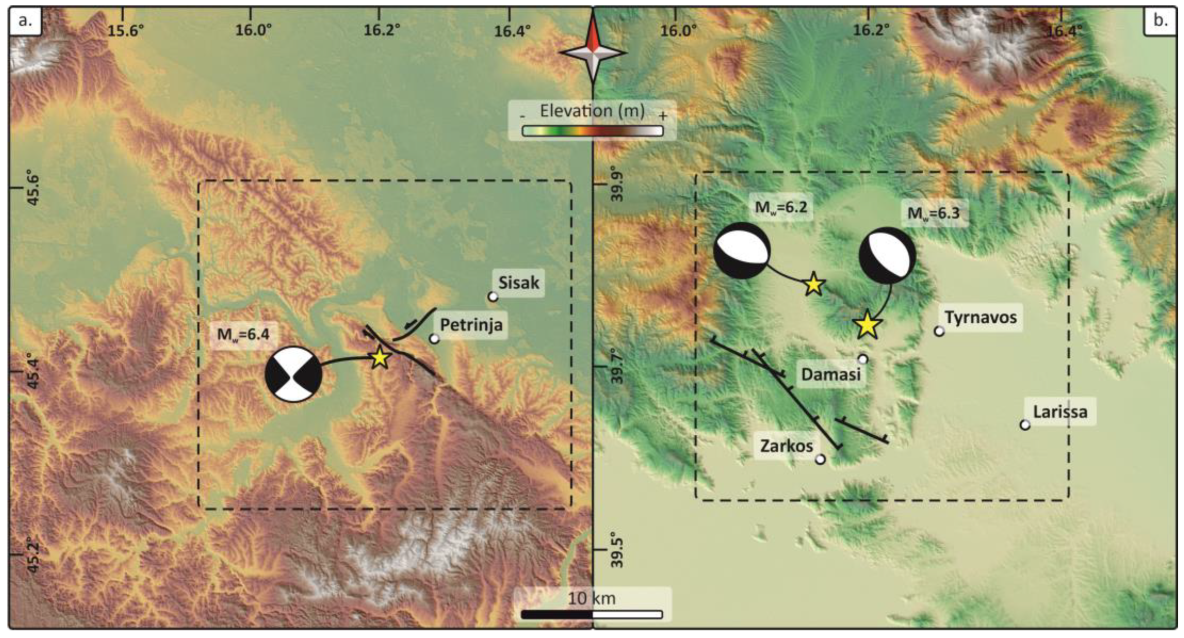
Figure 1). By choosing both cases, it is possible to validate the results in two different tectonic contests characterized by prevalently horizontal (Croatia) and vertical (Greece) coseismic movements.
The M
w 6.4 Croatia earthquake occurred on 29 December 2020 near the city of Petrinja, causing severe damage. The earthquake was triggered by strike-slip tectonics as indicated by the fault plane solution, including nearly vertical NW-SE and NE-SW trending nodal planes (
Figure 1a). Reference [
14] reports a detailed description of the deformation pattern associated with the Petrinjia earthquake, using both remote sensing (InSAR, Sentinel-1) and field data. Several important coseismic ruptures are observed and mapped in the field [
15], testifying to a typical conjugate fault pattern associated with the main NW-SE right lateral seismogenic fault. In [
18], a maximum displacement of ~43 cm along the E-W component, a maximum subsidence of −15 cm and an uplift of +19 cm are also reported.
The 2021 Greece earthquake sequence occurred in the Thessaly region and was characterized by three mainshocks [
19], with a predominantly extensional kinematics, representing the westward propagation of Tyrnavós graben [
20] (see focal mechanisms of
Figure 1b).
Figure 1.
Simplified seismotectonic map of (
a) the M
w 6.4 Petrinja earthquake in Croatia (29 December 2020) and (
b) the M
w 6.3 and M
w 6.2 Tyrnavos earthquake in Greece (3–4 March 2021). The activated seismogenic faults (black lines with kinematic indicators) and the focal mechanisms are from [
15] for the Croatia earthquake and from [
20] for the Greece earthquake. The base map is a composite of DEM and Hillshade derived from the NASA SRMT DEM.
The seismic sequence was studied using InSAR and seismic data by [
19,
21]. Ref. [
19] reports a detailed coseismic displacement map due to the M
w 6.4 event inferred by InSAR data. Following these authors, the sequence started with a M
w 6.3 event that occurred along a NE-dipping normal fault segment striking N314 at a depth of ~10 km, which produced a ground subsidence of ~40 cm. The second event (M
w 6.2) occurred in the NW along a further parallel fault segment at a depth of ~7 km, producing an estimated ground subsidence of ~10 cm. Most likely, the same fault was ruptured further to the NW on 12 March (M
w 5.7) at ~10 km depth. Ref. [
19] reports that three blind normal fault segments were activated during this seismic sequence, the entire system of which forms a graben-like structure in northwest Thessaly. This work is focussed on the cumulative deformation of the two first mainshocks (3–4 March 2021), using a dataset with a sensing period going from 24 to 25 February to 8 to 9 March 2021.
3. Methods and Data
3.1. Differential Synthetic Aperture Radar Interferometry (DInSAR)
Differential Synthetic Aperture Radar Interferometry (DInSAR) is a method of calculating the phase difference between a pair of SAR images, which consists of a primary image, usually acquired before the occurrence of a precise event, and a secondary image, referred to as a period consequent to the occurrence of the event. The two images, moreover, referred to the same target area on Earth’s surface. The resulting product represents a measure of the ground displacement projection along the line of sight (LOS) of the sensor [
1]. This is made possible by removing the topographic phase from the interferogram since the phase is correlated to topography and by unwrapping the phase contained in the interferogram. This will provide a metric value to the phase and the real change in Earth’s surface during the time interval between the two acquisitions.
The DInSAR technique is largely exploited in many Earth science fields, such as, for example, landslide monitoring [
7,
22,
23,
24], land subsidence [
7,
25,
26] and volcanic environment problematics [
27,
28,
29,
30].
A further key issue of the DInSAR technique is the coherence, an index that indicates the quality of the phase information and the similarities between the two images. Its value varies from 0 to 1, where 0 is referred to as the lowest value of coherence, and 1 is the highest. Coherence losses may derive from different factors, summarized as follows:
Geometric factor: for a change in the look angle that could be amplified by the presence of slopes toward the radar;
Land factor: occurrence of landslides, floods, volcanic eruptions that have modified the morphologic aspect of the land surface and the presence of water;
Vegetation factor: the presence of rainforests or other types of vegetated areas;
Temporal decorrelation: caused by modifications that occurred on the surface of the scattering targets during the time interval between the acquisitions of the images;
Differences in the satellite orbits between two different passages.
Despite these issues, DInSAR technique can be considered a powerful method for the detection of Earth surface displacements in short time ranges. The centimetric resolution of the final data is a fundamental piece to the completion of on-field observations in Earth sciences. More details about the theory and processing steps of this method are reported in “
Appendix A”.
DInSAR processing can be executed by using specific software or internally developed codes. One of the most exploited open-source software to perform the DInSAR processing chain is the SentiNel Application Platform (SNAP), whose main advantage consists of the Sentinel-1 toolbox; it supplies all the operators able to perform DInSAR processing, including the algorithm for the phase unwrapping (SNAPHU). The latter is a crucial operation, which represents the base processing step to convert the phase, expressed in cycles of π, into displacement, expressed in meters (more details in
Appendix A). Thanks to these tools and to the open-source character of the software, data processing via SNAP has been adopted for different applications, such as earthquakes [
31,
32], land subsidence [
33,
34], polarimetry [
35] and flood mapping [
36,
37].
3.2. SNAP Software
The SeNtinel Application Platform (SNAP,
https://step.esa.int/main/download/snap-download/, accessed on 15 November 2023) is an architecture provided by ESA and developed by Brockmann Consult, SkyWatch and C-S (ESA), built for Earth observation processing and analysis. SNAP provides (i) a very fast image display and navigation even of giga-pixel images, (ii) a Graph Processing Framework (GPF) for the creation of a processing chain that is customizable by the user, and (iii) an automatic DEM download and tile selection or layer management instruments [
38] (
https://step.esa.int/main/toolboxes/snap, accessed on 15 November 2023). The main advantage of such software is the open-source character and the capability to contain all the Sentinel toolboxes that can perform the processing of every dataset from both ESA satellites and third-party missions (e.g., for SAR missions, TerraSAR-X, Cosmo SkyMed).
3.3. Python Implementation
Parallel to the development of software for data processing is the development of personal scripts with the same finalities. The scripts have a more flexible customization; nevertheless, it is necessary to have proper skills in programming to create an efficient and powerful tool that could satisfy any request for precise processing. In the specific case of the DInSAR technique, the versatility of creation of these tools has led to the development of various scripts (GMTSAR [
39], DORIS [
40] or ISCE by NASA Advanced Information Systems Technology), helping the scientific community significantly in strengthening knowledge on the method.
This work takes advantage of the existence of a Python module called snappy, which is provided by SNAP software. Through the combination of such modules with packages and libraries present in Python, a new script called Snap2dQuake is developed to allow any user to work with the DInSAR technique on Sentinel-1 data. The script covers all the main processing steps, from the split of the SAR images to the computation of the LOS (along both ascending and descending orbits), E-W and vertical displacement maps.
Snappy is a Python module available with SNAP, which can be easily configured during the installation of SNAP, and it is composed of all the operators belonging to each toolbox furnished by SNAP. The users have the possibility to customize their own processing by creating a personal Python script, which can be improved with the insertion of other Python operations derived from other libraries and modules. This type of customization represents a great advantage, largely due to the possibility of avoiding the graphic interface of SNAP, speeding up the overall data processing. Another advantage is the possibility to automatize the processing, thus overcoming some of the problematic operations on SNAP software. One of them is the Enhanced Spectral Diversity, which, sometimes, cannot be performed correctly on SNAP, preventing the process in the work chain. This problem and similar problems have been solved with Snap2DQuake by using a library in Python, which allows the creation of .xml files reproducing the actions of the operators, overcoming the software bug. Furthermore, although the Graph Constructor tool of SNAP software allows partial automatization, some operators cannot be smoothly inserted, such as the SNAPHU Unwrapping. To run the operator in SNAP, the user must proceed with two separate commands: SNAPHU export and SNAPHU import. With Snap2DQuake, the two operators are automatically run.
The reproduction of all the operators in a single script can overcome the SNAP issues and automatize the entire data processing. The user only needs to select the data input and set the necessary values before running the script. The automatic character of this technique is strongly relevant because it allows beginner users new to coding, interferometry and the DInSAR technique to rapidly obtain deformation maps from the raw data. Snap2DQuake is developed to automatize the entire DInSAR workflow, overcoming the bugs and issues that can occur during the processing with the SNAP software.
Nevertheless, the authors are keen to clarify that the presented Snap2DQuake tool is not intended to represent an innovation or replacement of SNAP software but rather a new and simple solution that is mostly designed for basic users of DInSAR and Python to process Sentinel-1 data and obtain reliable displacement maps without necessarily interacting with the software and its possible complications.
The proposed Python script is available in the “Data Availability Statement” section.
3.4. SAR Sentinel-1 Data
The SAR data used for this work consist of Sentinel-1 single-look-channel interferometric wide swath products. The interferometric wide (IW) swath mode is the main acquisition mode over land for Sentinel-1 and allows for the acquisition of data with a 250 km swath at 5 m × 20 m spatial resolution in range and azimuth, respectively (single look) [
41,
42]. Such a high geometric resolution is possible thanks to the implementation of the IW mode with the Terrain Observation by Progressive Scan (TOPSAR) operation [
43], with which the beam electronically transmits a burst of pulses backward to forward in the azimuth direction for every sub-swath. The IW products can acquire SLC (Single-look Complex) images (swaths) that are characterized by three sub-swaths (IW1, IW2 and IW3) per polarization channel for a total of three or six images (depending on whether it is a single or dual polarization). In an IW product [
41], there are a series of bursts in the azimuth which partially overlap to obtain continuity in the image; each burst is processed as a separate image.
The data, derived from Sentinel-1, have been downloaded from the Copernicus Open Access Hub, now Copernicus Browser [
44], and are referred to as both ascending and descending orbits (see
Table 1 for further details).
4. Description of the Processing Workflow and Structure of Snap2DQuake
The workflow adopted to generate a surface displacement map, such as an area affected by a strong earthquake, consists of different steps that are summarized in this section. The final product is not only the displacement along the line of sight (LOS) of the satellite but also the displacement in the horizontal (E-W) and vertical directions. The absence of information along the north direction is motivated by the near-polar orbit of the satellite, for which the north–south displacement verifies a direction that is almost parallel to the satellite orbit and quite difficult to extract. The workflow, applied to a couple of images named primary and secondary (e.g., before and after a seismic event, respectively), can be summarized in the following steps (
Figure 2):
Figure 2.
Schematic description of the processing structure of Snap2DQuake.
Figure 2.
Schematic description of the processing structure of Snap2DQuake.
This first part of the workflow is applied to primary and secondary images for both ascending and descending orbits to obtain LOS displacement maps and, subsequently, by combining the resulting products, the horizontal and vertical displacement maps. This second part of the workflow can be performed with two different approaches:
The usage of one operator instead of the other depends on the user’s preference:
BandMaths allows one to mathematically interact with the data, while
Horizontal/Vertical Motion directly calculates the horizontal and vertical displacement starting from the ascending and descending data input. In this work, the E-W and vertical displacements have been calculated using
BandMaths, with the aim to test the reliability of the mathematical approach proposed by [
6] for the E-W and vertical components retrieval (
Appendix A). Since the formulation is made on geometric assumptions, the results can be approximated. In this work, we adopt the approach by [
6] by comparing our results with those proposed in the literature.
5. Results
5.1. Interferograms, LOS and Displacement Maps
In this section, we present the results obtained by running the Snap2DQuake tool. The DInSAR interferograms and LOS displacement maps for the M
w 6.4 Petrinja and the M
w 6.3 and M
w 6.2 Tyrnavós earthquakes are shown in
Figure 3 and
Figure 4, respectively. The coseismic deformation patterns for the two earthquakes are described by displacement maps of vertical and E-W components (
Figure 5 and
Figure 6). The details of ground deformations are described by displacement variations along two sections passing through the main faults, which are produced using the Q-GIS plugin Terrain-profile (
Figure 5c,d and
Figure 6c,d).
5.1.1. Petrinja Earthquake (Mw 6.4, 29 December 2020)
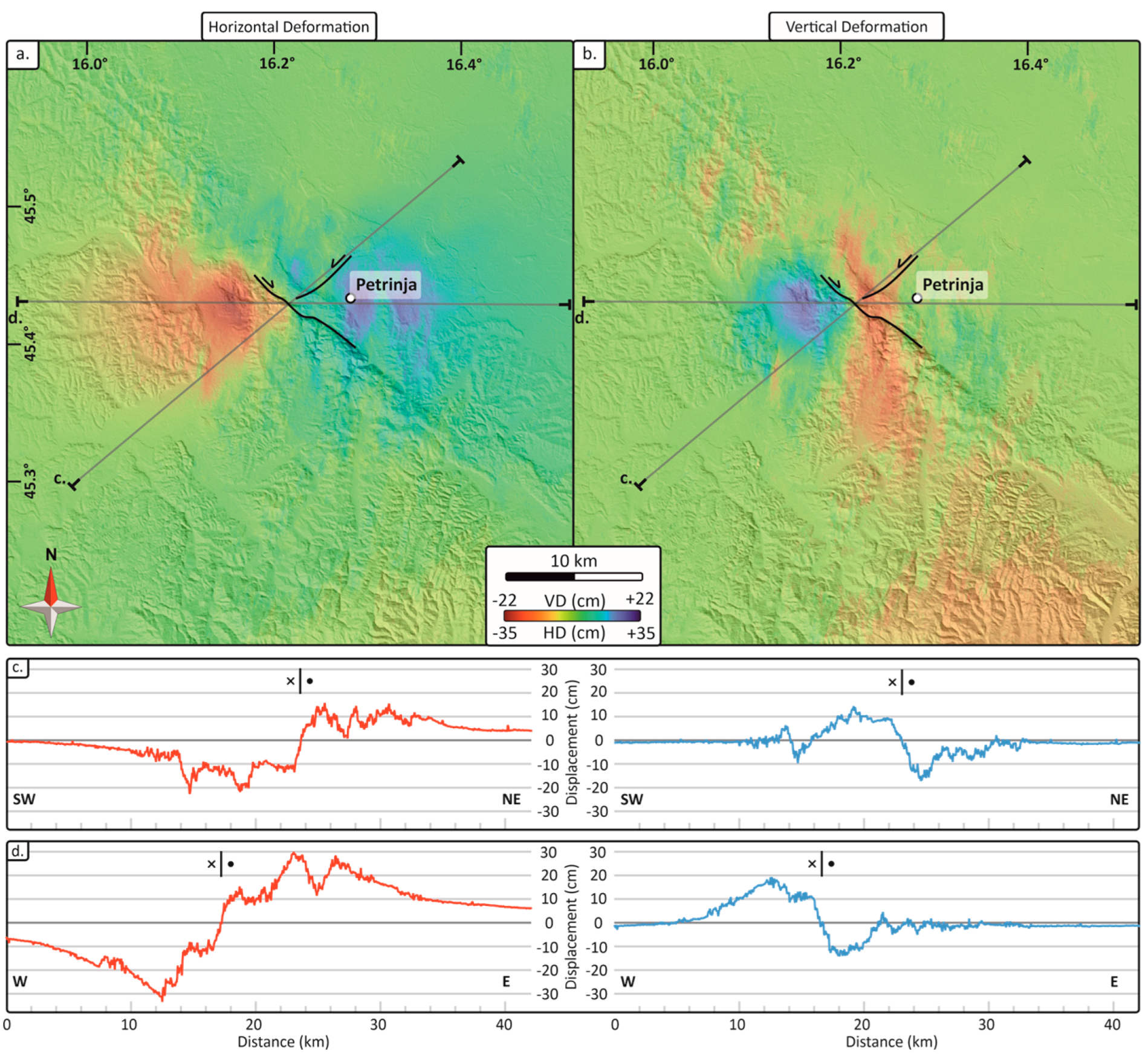
The Croatian Mw 6.4 earthquake is characterized by a strike-slip right movement and, consequently, by a prevalent horizontal displacement; the E-W component is thus expected to contain higher values of displacement than the vertical component.
The dataset is constituted by a couple of ascending orbit products from Sentinel-1A, with primary acquisition on 18 December 2020 and secondary acquisition on 30 December 2020, and by a couple of descending orbit products from Sentinel-1B, with primary acquisition on 23 December 2020 and secondary acquisition on 4 January 2021 (
Table 1).
The differential interferograms for both orbits show a similar E-W elongated elliptical shape, with a thickening of the fringes in the area close to the fault (
Figure 3a,c). The LOS displacement seems to be better resolved for the ascending (
Figure 3b) than the descending orbit (
Figure 3d). The obtained E-W and vertical displacement maps (
Figure 5) show the distribution of the deformation promoted by the mainshock. The area with the highest westward movement (to the left side of the fault, red area in
Figure 5a) also corresponds to the area with the highest uplift (blue area in
Figure 5b). The area affected by the higher eastward movement (blue area, right of the fault in
Figure 5a), which is wider and more distributed, does not exactly correspond with the highest subsidence (red area in
Figure 5b), which instead is constrained closer to the activated fault. The horizontal (E-W) movement is by far the most critical component, affecting about 440 km
2 with a maximum displacement of ~34 cm. On the other hand, the vertical displacement only affects about 220 km
2, with a maximum subsidence of ~19 cm and a maximum uplift of ~21 cm.
The variation of the displacement values is also shown in the profiles along two orientations: one is oriented orthogonally to the average strike of the structure (
Figure 5c), while the other is oriented in the E-W direction (
Figure 5d). While the first intercepts the area with the higher amount of subsidence, the latter is oriented to fit the areas with the higher amount of E-W movement at both sides of the fault. The orthogonal profile shows that the horizontal movement is not always correlated to a vertical deformation; the latter, in the right block, is close to 0 cm and already a few km away from the fault, while the horizontal movements show values from around 5 cm (
Figure 5c) to ~30 cm (
Figure 5d). It is also possible to identify the location of the main fault using the orthogonally oriented section (
Figure 5c) for the E-W component. The fault is easily recognized where there is an abrupt transition from westward to eastward deformation (see transcurrent symbol in
Figure 5c,d). The short wavelength irregularities of the deformation profiles suggest a mid-rumor for the signal, which, however, does not impede the discernment of a detailed distribution of the displacement, as well as the location of other secondary and conjugate faults in agreement with [
15]. Moreover, according to the deduction reported by [
15] from field observation, we also detect the presence of an NNW-SSE trending subsided sector (
Figure 5d), in agreement with normal faults in a conjugate Riedel shear of strike-slip tectonics.
5.1.2. Tyrnavós Earthquakes (Mw 6.3 and Mw 6.2, 3–4 March 2021)
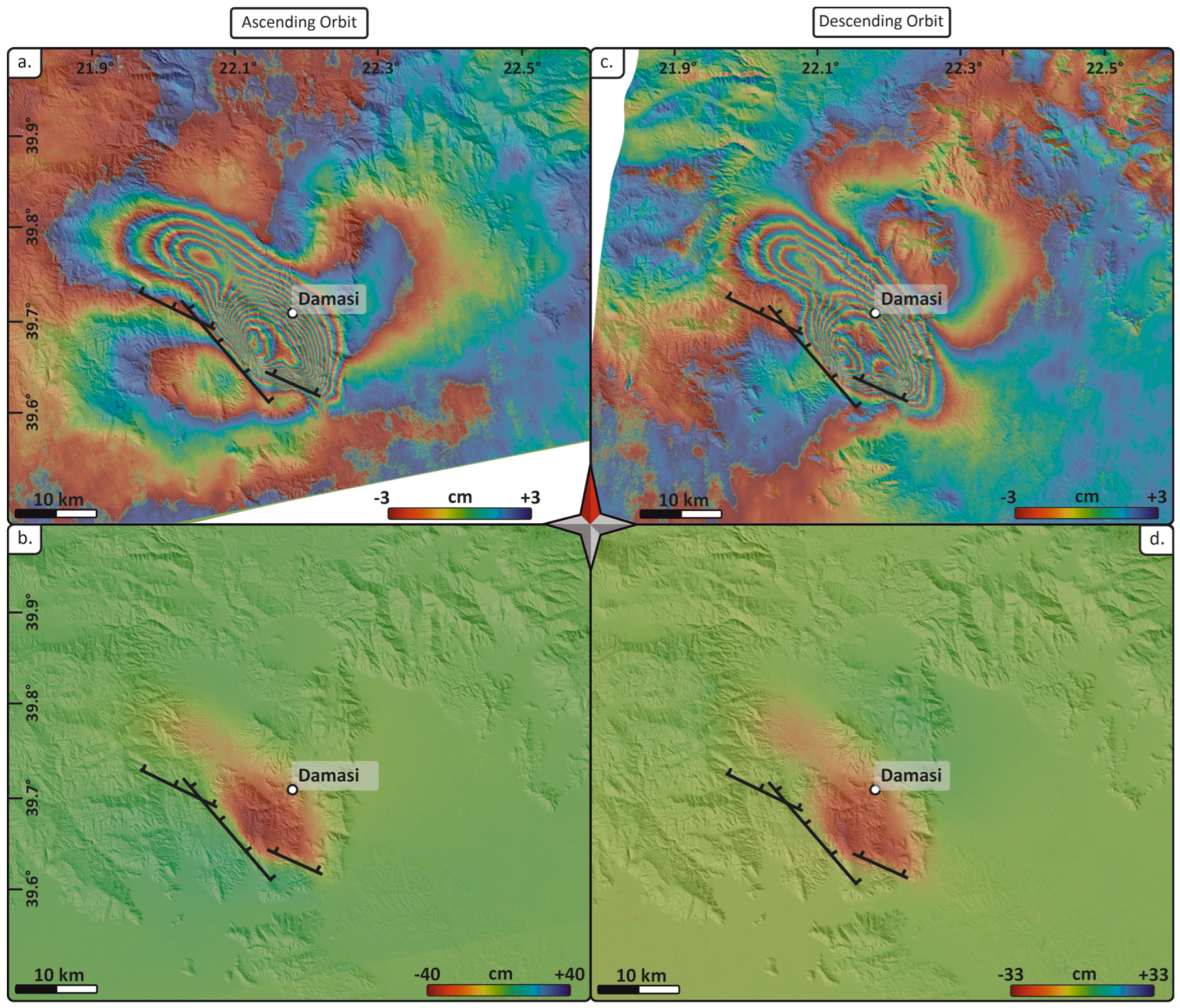
The Greek earthquake sequence is characterized by a prevalent extensional tectonic regime, thus a prevalent vertical motion. For this case study, the adopted dataset is characterized by a couple of ascending and descending products from Sentinel-1A, with primary acquisition on 25 February 2021 and secondary acquisition on 9 March 2021 for the ascending orbit and primary acquisition on 24 February 2021 and secondary acquisition on 8 March 2021 for the descending orbit (
Table 1).
The differential interferograms for both orbits show a well-defined NW-SE elongated elliptical shape, with two main lobes (at SE and NW), following the trend of the fault segments for the event of 3 and 4 March 2021 (
Figure 4a,c), of M
w 6.3 and M
w 6.2, respectively. The LOS displacement maps show the same ground deformation pattern for ascending and descending orbits (
Figure 4c,d). The E-W and vertical displacement maps obtained through our approach (
Figure 6a,b) show the cumulative distribution of the two components of the deformation that occurred during the seismic events. The vertical displacement (
Figure 6b) is very well constrained at the hanging wall of the activated fault, within an area of about 210 km
2 characterized by a subsidence of up to ~44 cm. We do not observe a significant uplift component, not at the footwall nor to the northeast of the subsided hanging wall. The E-W component (
Figure 6a) is more widely distributed within an area of about 630 km
2 and is not only limited to a relatively small area close to the fault. However, the highest movement of 20 cm is to the east and located at the hanging wall (
Figure 6a), while a slight movement to the west with the highest value of ~17 cm is observed, which is located at the southern part of the hanging-wall block (
Figure 6a).
Also, in this case, a section orthogonal to the average strike of the inferred fault (
Figure 6c) was traced to fit the highest amount of vertical displacement (subsidence in this case), and a second section that is E-W-oriented (
Figure 6d), crossing the area with the highest amount of horizontal (eastward in this case) movement. From the deformation profiles along the sections, it is clear how the horizontal and vertical movements can be associated with a NW-dipping normal fault, as indicated by the presence of a well-defined subsided block, which also corresponds to the highest eastward horizontal movement. The fault responsible for the mainshock can be easily identified using the orthogonally oriented section traced on the vertical displacement map (
Figure 6c,d). In this case, the subsided block is characterized by a steep northeast-dipping slope (very close to the fault) and by a shallower, bent southwest-dipping slope at the hanging wall. However, we do not observe an uplift at both sides of the fault, which is also characterized by a widely distributed, even if low, horizontal movement, which is also far from the activated fault (black arrows in
Figure 6c,d). In addition, the profiles of this case study show a very low rumor of the signal, guaranteeing a clean interpretation of the actual deformation.
6. Discussion
6.1. Snap2DQuake Reliability
The comparison of the presented results with the outcomes from previously published works, using the same time intervals, allows us to define the reliability of the proposed approach. This comparison is motivated by the computation of the E-W and vertical components in Snap2DQuake, which is based on the assumptions by [
6]. The latter is different from the computational system behind the
Horizontal/Vertical Motion operator of SNAP software. The comparison is performed through a simple observation of the LOS and the two components’ displacement maps, followed by a quantitative evaluation of the displacement (in cm) derived from the DInSAR dataset.
Table 2 reports the maximum horizontal and vertical displacement values obtained from the literature and from this work, as well as the difference between the two datasets.
The results from Snap2DQuake for the Petrinja earthquake are compared with the results by [
15,
18]. While [
18] reports both ascending and descending orbit LOS displacement, [
15] only reports ascending orbit LOS displacement; thus, the latter is used only for comparing the ascending orbit. The comparison shows a small difference in the displacement pattern but the same values of displacement. Since the processing methods are the same, such a result was expected. The comparison was needed to check if the outputs from Snap2DQuake can be considered valid and without errors, considering that the script runs the operators without the direct
snappy tool but with alternative solutions consisting of external executable files. For the horizontal and vertical components of displacement, the presented resulting maps show approximately the same values as in [
18]. In particular, the difference along the horizontal component is 9 cm (E component) to 11 cm (W component), whereas the difference along the vertical component is 2 cm (up) to 4 cm (down) (
Table 2). Those differences are motivated by the usage of the method of [
6], which is based on geometric assumptions. Nevertheless, the pattern of the deformation obtained in this work is still comparable with data collected in the field by [
15] for the E-W component.
Such a good match demonstrates the reliability of the method proposed by [
6] for the retrieval of the horizontal and vertical components. The slight difference in the pattern of deformation for each component is reasonable based on the mathematics behind the method, following the approach of [
6]:
Since the E-W and vertical displacement maps derive from the combination of both ascending and descending products and since the pattern of the descending displacement map differs from the one reported in [
18], it is obvious that the E-W and vertical displacement maps are also expected to contain some differences in the pattern of displacement. However, it is important to underline that the crucial factor allowing the establishment of the reliability of a product is the value of the displacement, which is considered good if it fits the values of displacement obtained from field measurements [
15].
Regarding the case study of the Tyrnavós earthquake, the comparison of the presented results with the work by [
19] shows a very good agreement in the LOS displacement maps for both ascending and descending orbits. Regarding both the E-W and vertical displacement maps, our approach, integrated with the method by [
6] for the retrieval of the horizontal and vertical displacements, also produces comparable results; indeed, the displacement maps from Snap2DQuake show values completely comparable with those previously published (see Figure 16 in [
19]). In detail, the difference along the horizontal field is only 1 cm along the E component and 8 cm along the W component, whereas along the vertical component, the difference is from 4 (down) to 6 cm (up) (
Table 2).
The matching of maximum displacement values along both components (horizontal and vertical) for the two considered case studies demonstrates the high reliability of the proposed workflow. The deformation pattern provided by displacement maps is well resolved and allows us to constrain the location and the geometry of the main seismogenic faults, as well as those of minor faults and ruptures associated with complex deformation (as in the case of the Croatian strike-slip earthquake).
The obtained horizontal and vertical displacement maps are recognized to be very useful for applications in seismotectonic studies. Indeed, the detailed patterns of coseismic deformation retrieved by displacement maps can be useful to map the tectonic features involved in the seismic event while also suggesting the likely mechanism behind the earthquake. This latter information can be easily derived by analyzing the displacement maps referred to as the E-W and vertical components. High values in the vertical field can suggest a dip-slip mechanism, while high values in the E-W field can suggest a prevalence of a strike-slip mechanism. In addition, it would be eventually possible to recognize the associated transpressive or transtentional component. Therefore, a simple previous analysis of the displacement maps can provide significant help in mapping tectonic elements during the on-field observations.
6.2. Snap2DQuake Advantages, Limits and Processing Suggestions
The proposed Snap2DQuake script, constructed as an open-source tool integrating the snappy module by SNAP software and Python packages and libraries, is validated by DInSAR data from previous studies. However, questions about the performance and convenience of using this Python script that reproduces the same operators of SNAP software can be raised.
The first answer lies in the substitution of the operators that present issues in SNAP software (e.g., the Enhanced Spectral Diversity operator) with the combination of other operations furnished by libraries and packages of Python. This helps in the construction of structures in such a way that the issue of that precise operator can be overcome and solved in an alternative way.
An additional advantage is the automaticity of the proposed script, for which the general workflow results are accessible even to beginner users of both programming and DInSAR processing. The only features to interact with are (i) the insertion of the datasets and of the paths where the files should be stored, (ii) the values of the parameters for the interferogram formation, the Multilook and the filtering, and (iii) the insertion of the Area of Interest (AOI) coordinates. These operations do not require any programming skills since they just involve the insertion of values and data paths. Moreover, the script contains all the necessary information to know which values the user must insert and how to generally interact with the overall code.
Another advantage of using Snap2DQuake is the possibility to insert the phase unwrapping operation in the entire processing, which is not possible with the Graph Constructor operator using the SNAP software; consequently, the presented Python script helps with the automatization of the workflow. In addition, the writing of each single product from the operators is not mandatory when using Snap2DQuake, and this strongly accelerates the entire work chain. Avoiding the usage of the graphical interface of SNAP, the DInSAR data processing in Python results in a rapid method to obtain displacement maps in shorter times than with the SNAP software. However, it is important to report that the SNAP software is in continuous development, and during upgrading, some operators may not be performative with Snap2DQuake nor with snappy on Python and the SNAP software.
In general, the application of the DInSAR method is strictly constrained by the case study being analyzed; due to the intrinsic limits of the SAR data, the technique cannot be very performative if applied on earthquakes characterized by excessive magnitude (e.g., >7.5 Mw) and/or occurring in a highly vegetated environment.
Considering the limits of the DInSAR method, during the comparison between displacement maps obtained from different processing, it may happen that, even using the same dataset, the resulting displacement maps present differences in the distribution of the deformation pattern. The explanation may lie in the different types of processing and/or in the values inserted during the interferogram formation and the speckle filtering processes. During the interferogram formation, it is crucial to choose a good size for the coherence estimation window; from a scenario characterized by medium to low coherence values, a good interferogram can be derived if the window size is large enough to calculate both the phase and the coherence while not losing a significative amount of resolution. During such an operation, the parameters of the filtering process must be chosen so that the final product can still be reliable for the following steps of the workflow. In the case of the application of the Goldstein filter to an interferogram calculated with a large coherence estimation window, the more appropriate value of FFT size is a high value applied on a small window; for example, SNAP allows the user to choose between four different values—32, 64, 128 and 256. More details about these operators are reported in
Appendix A.
7. Conclusions
The present work is aimed at proposing and delivering an approach based on the exploitation of the snappy module of the SNAP software (ESA). Such an approach consists of an open-source, automatic and simple tool that rapidly performs the DInSAR work chain to obtain LOS displacement maps (along both ascending and descending orbits) and the ground displacement along both horizontal (i.e., E-W) and vertical components. The choice to simulate the operators proposed in SNAP software’s Sentinel-1 toolbox allows some limitations of the SNAP software to be overcome and for the furnishing of a user-friendly and automatic too.
The retrieval of E-W and vertical displacements involves applying the method proposed by [
6].
The results from the proposed tool are compared with previously published displacement maps for the same case studies. The accordance of the results ensures the reliability of the alternative introduced operators and actions, together with the proof of how this tool can represent an alternative to obtain reliable maps with zero costs.
The proposed Snap2DQuake script can be significant for basic users of DInSAR, SNAP software and programming, with minimum effort in both costs and Python knowledge. The user of this tool will be able to rapidly obtain exhaustive displacement maps that can be constrained with on-field analysis and/or that can furnish fast information on the deformation field referring to areas affected by seismic events or by other phenomena involving ground deformation. It is important to remember, however, the limits of the method, which are strictly reduced to problems of developing the software itself. In addition, it is necessary to remark that Snap2DQuake is not aimed at providing alternative processing of Sentinel-1 data with the same tools of SNAP software but at avoiding some SNAP limitations. The authors want to underline that DInSAR deformation maps must not be considered a substitute for field analysis, but they can be crucial for a better definition of the deformation field thanks to the centimetric resolution of the products and the fast delivery time.
Author Contributions
Conceptualization, M.O., M.P., S.A., N.P. and C.L.-M.; methodology, M.O.; software, M.O.; validation, M.O., F.C., C.L.-M. and M.P.; formal analysis, M.O. and C.L.-M.; investigation, M.O. and F.C.; resources, M.O., F.C. and M.P.; data curation, M.O. and F.C.; writing—original draft preparation, M.O. and M.P.; writing—review and editing, F.C. and M.P.; visualization, F.C.; supervision, M.P.; project administration, M.O. and M.P.; funding acquisition, M.P. All authors have read and agreed to the published version of the manuscript.
Funding
This research was funded by Ministero dell’Istruzione dell’Università della Ricerca (MUR) through the program PON “Ricerca e Innovazione” 2014–2022, the ASI-UniPG agreement 2019-2-HH, Fondo Ricerca 2022 Dip. Fisica e Geologia dell’Università di Perugia “A new approach to detect ground deformation after large earthquakes using open-source DInSar data” (RIC-BAS2022PORRECA) and Fondo Ricerca Ateneo 2021 (WP3.1 “Disastri e Crisi Complesse).
Data Availability Statement
The proposed Python script is freely available to the entire scientific community through the link reported below this paragraph. With the code, the authors also make available the Python environment in which to run the script and a series of .xml files for the execution of some operators, allowing users to avoid any potential issues by utilizing snappy. The execution of these operators, as with the entire script, is completely automatic: the only parts of interactions between the user and script are the insertion of the input data, the file destination folders and the paths where the .xml files are located. The code is in continuous development to improve the efficiency of the overall processing and to update eventual operators, and every update will be uploaded at the same link reported in this section. The authors are available for eventual clarifications about the products as well as for further implementations of the script. Link to the code “Snap2DQuake” on Github:
https://github.com/navre6/Snap2DQuake (accessed on 15 November 2023).
Acknowledgments
The authors are grateful to A. J. Camps (Universitat Politécnica de Catalunya, Barcelona), C. De Luca (CNR-IREA, Naples) and M. Petrelli (University of Perugia) for their support in the writing of the presented work. The authors would also like to thank the European Space Agency (ESA) for providing SAR images of Sentinel-1.
Conflicts of Interest
The authors declare no conflict of interest.
Appendix A
Appendix A.1. Coregistration
To better understand the base principles of DInSAR, it is important to remark that in a SAR image, each pixel contains two types of information: wave amplitude and phase. The phase is the sum of [
45]
where φspec is the specific phase and describes the interaction between wave and land, being related to the physical nature of the land and to the look angle; φD describes the propagation wave, whose phase increases by 2π every time the wave crosses a distance equal to the wavelength. This effect can be defined with the following relation [
45]:
where D represents the range from the source to the center of the pixel.
Considering these previous assumptions, the formation of the interferogram consists of cross-multiplying the reference primary image with the complex conjugate of the secondary image. The amplitude of both images will be multiplied, while the resulting phase will represent the phase difference between the two images; the latter represents a different travel path from the source to the land [
39]. The computed phase is the sum of several contributing factors [
41]:
where Φdem = −(4πλ)·(B
ns/Rtanθ) is the topographic phase of the Earth’s surface, φflat = −(Δq/sinθ)·(B
n/R)·(4πλ) is the Earth’s curvature (or the flat-Earth phase), and φdispl = 4πλ is the deformation between the two acquisitions. Since the main goal of the DInSAR technique is to define the elevation changes between the two acquisitions, and φatm+φnoise is considered as small as possible, (A3) can be written as
which is the final equation for the interferogram formation.
Appendix A.1.1. TOPSAR Split
TOPSAR Split operator is applied to the SAR image to select only the necessary bursts from a sub-swath for the analysis. The dataset usually contains a great amount of pixels (and so, information); thus, processing the entire image could take an unnecessarily long time. The S-1 TOPSAR Split operator allows the selection of one of the three sub-swaths (IW1, IW2, IW3) and polarization (VH or VV), as well as bursts (1 to 9). The number of bursts to select depends on the location of the epicenter and on the possible extension of the impacted area. A small number of selected bursts will lead to faster data processing since the data load is low; however, it will not necessarily cover the entire field of deformation. This operator is performed two times to apply it on both primary and secondary images.
Appendix A.1.2. Application of Orbit Information
This operator is applied to a split product to add the orbital information to the data, which consists of auxiliary data that furnish the position of the satellite during the acquisition of the data. These data files are directly and automatically downloaded in SNAP and are available for both SNAP software and snappy module for Python. As for the TOPSAR Split operator, the Apply Orbit File operator must also be executed separately on the primary and the secondary images.
Appendix A.1.3. Back Geocoding and Enhanced Spectral Diversity
The Back Geocoding operator performs the process of co-registration of the two image splits after the application of the orbit information. To increase the quality of the dataset, the Enhanced Spectral Diversity operator applies range and azimuth corrections.
Appendix A.2. Interferogram Formation
The process of interferogram formation is a fundamental step that allows the use of phase information to extract distance variations from the satellite and the Earth’s surface. In SNAP, the interferogram formation is performed by an operator that contains both flat-Earth and topographic phase removal with the coherence estimation. The resulting product is the interferogram, with information on the relative altitude and coherence, where dark areas refer to loss of coherence. These products are generated as separate sub-products of the same product, which in SNAP are called bands. In order to reduce loss of coherence in the product, the window size for coherence estimation can be changed: larger windows derive products with enough coherence to perform DInSAR but with loss of resolution.
Appendix A.3. TOPSAR Deburst, Multilook, Phase Filtering and Subset
The products resulting from the interferogram formation contain some seamlines between the bursts, which are removed with the subsequent step using the TOPSAR Deburst operator.
Once the product is debursted, the image still presents a different spatial resolution in range and azimuth directions, and the pixels’ geometry appears rectangular. The Multilook reports the geometry of the pixels in such a way that it could be representative of the ground, which means that the resulting geometry in range and azimuth must present a 1:1 ratio.
After the application of the
Multilook, the product is presented as deeply granular because of the presence of noise. The noise is due to temporal decorrelation caused by the time span between the two acquisitions and due to geometrical decorrelation caused by the motion of a reference target P from one position to another in the time interval between the two acquisitions. They can be reduced by shortening the acquisition time interval (e.g., choosing two consecutive acquisitions) and by geometric correlation. To further reduce the noise,
Phase filtering has to be applied to the image. The presented workflow chooses the Goldstein filter [
46] since SNAP furnishes an operator that performs the same filtering type. According to [
46], the interferogram is segmented into two overlapping rectangular patches for which the power spectrum is computed, smoothing the intensity of the two-dimensional Fast Fourier Transformation (FFT). The response of the filter is [
46]
If the value of the filter parameter α = 0, no filtering occurs, while if α = 1, the filtering is strong. The choice of the value for α strictly depends on the case study: useful values of α lay between 0.2 and 1, and high values with large patch sizes are more appropriate for low coherence interferograms. The Goldstein filter applies the FFT to enhance the signal-to-noise ratio of the image.
Since the data can still be big and heavy, the Subset step allows the choice of a smaller AOI, reducing the output size and accelerating further processing steps. The operator Subset allows the cutting of the image with a precise window that is customizable by the user. The choice of window size can be expressed in both pixels and coordinates (longitude and latitude).
Appendix A.4. Phase Unwrapping
The output product from the Goldstein filtering is an interferogram that furnishes information on the altitude. However, the measurement of the terrain altitude in the interferogram is ambiguous, and it is due to the cyclic nature of the interferometric phase. The variation of the interferometric phase varies from −π to +π and corresponds to an entire cycle of 2π, which is referred to as a color cycle in an interferogram. The interferometric phase change of 2π is defined as altitude of ambiguity, and it can be solved by unwrapping the phase. This consists of relating the interferometric phase to the topographic height and adding (or deleting) the correct integer multiple of 2π to the interferometric fringes [
41,
47]. Given that P represents every pixel composing the image, and ϕ(P) is the exact phase value [
45],
where φ(P) is the phase value before the phase unwrapping. Unwrapping the phase means obtaining the geometrical parameters from the correlation between height and phase. However, the process can be compromised by inherent noise coming from the system or by large deformation gradients that can cause severe deviations in the process of unwrapping [
48]. The product resulting from the unwrapping process depends on the coherence.
The performance of phase unwrapping in SNAP is possible thanks to an implementation of the software with the algorithm proposed by [
49,
50] called SNAPHU. The algorithm is based on a maximum posterior probability (MAP) approach, which introduces a methodology where an interferogram is partitioned and unwrapped in its single tiles. Subsequently, the interferogram is divided into independent reliable regions. In turn, they are subsequently assembled into a full unwrapped solution with an objective function whose minimization can provide a good approximation of the real unwrapped phase. The module of SNAPHU in SNAP is composed of three steps:
SNAPHU export converts the data into a format readable by SNAPHU since it is an independent software implemented in another software;
SNAPHU Unwrapping consists of the algorithm itself. During the processing, the raster is subdivided into smaller chunks (10 rows and 10 columns) for a total of 100 tiles to unwrap. This subdivision of the datum is a default operation of the software. Therefore, the time of the processing depends on the data load; thus, the bigger the data load, the slower the processing.
SNAPHU import converts the unwrapped phase back into the format compatible with SNAP by adding the metadata of the wrapped phase to the unwrapped product, which lacks geocoding and metadata.
Appendix A.5. Phase to Displacement and Terrain Correction
The Phase to Displacement tool provides a metric meaning to the unwrapped phase by translating the pixel values in meters. Given this assumption, a positive value of the pixel means an uplift, while a negative value of the pixel is related to a subsidence. The output product is similar to the unwrapped phase but with a metric value associated with each pixel. An additional operation that can be performed after the application of this operation is the creation of an absolute zero in the image. By doing so, all the areas where the displacement is assumed to be zero in the time interval between the two acquisitions will have a displacement value of zero. In this way, the product will have a reference value for the displacement, just subtracting from the image the displacement value of a random pixel chosen in an area where no displacement is expected. At this point, if working with only ascending or descending products is sufficient, the last step is the performance of the Terrain Correction operator, which converts the image into a map with coordinate system using a Digital Elevation Model (DEM) to correct the distortions caused by the SAR sensor. The DEM can be chosen in SNAP or downloaded externally from the available DEM database services.
Appendix A.6. East-to-West and Vertical Displacement
Finding the displacement field of a target area affected by a large seismic event means projecting the vector representing the LOS displacement for both ascending and descending orbits in the three-dimensional space [
6]. From the simplified scheme of Sentinel-1 orbits reported in [
6], the LOS from both ascending and descending orbits belongs to the east-Z plane, and the incidence angle θ is assumed to be the same for both ascending and descending geometries. According to what reported in [
6], the E-W and vertical displacement can be retrieved with only geometric considerations as already reported in Equations (1) and (2).
To apply a mathematical formula on SNAP, it is necessary to resort to the BandMaths, an operator that allows for mathematical interactions with every kind of product opened on SNAP. This allows the combining of different sub-products of the same product (bands) and the use of functions, symbols and constants. With the new update of SNAP (9.0.0), a new operator is available to automatically calculate the horizontal and vertical displacements (Horizontal/Vertical Motion). The operator works on terrain-corrected interferograms from ascending and descending products (that are correlated with the Correlation operator before the performance of Horizontal/Vertical Motion operator) and returns products with pixel values that are already converted in the metric unit (mm).
References
- Gabriel, A.K.; Goldstein, R.M.; Zebker, H.A. Mapping elevation changes over large areas: Differential Interferometry. J. Geophys. Res. 1989, 94, 9183–9191. [Google Scholar] [CrossRef]
- Massonnet, D.; Feigl, K.L. Radar interferometry and its application to changes in the Earth’s surface. Rev. Geophys. 1998, 36, 441–500. [Google Scholar] [CrossRef]
- Massonnet, D.; Rossi, M.; Carmona, C.; Adragna, F.; Peltzer, G.; Feigl, K.L.; Rabaute, T. The displacement field of the Landers earthquake mapped by radar interferometry. Nature 1993, 364, 138–142. [Google Scholar] [CrossRef]
- Fialko, Y.; Simons, M. The complete (3-D) surface displacement field in the epicentral area of the 1999 Mw 7.1 Hector Mine Earthquake, California, from Space Geodetic Observations. Geophys. Res. Lett. 2001, 28, 3063–3066. [Google Scholar] [CrossRef]
- Stramondo, S.; Cinti, F.R.; Dragoni, M.; Salvi, S.; Santini, S. The August 17, 1999 Izmit, Turkey, earthquake: Slip distribution from dislocation modelling of DInSAR surface offset. Ann. Geophys. 2002, 45, 1–10. Available online: http://hdl.handle.net/2122/604 (accessed on 15 November 2023). [CrossRef]
- Manzo, M.; Ricciardi, G.P.; Casu, F.; Ventura, G.; Zeni, G.; Borgström, S.; Berardino, P.; Del Gaudio, C.; Lanari, R. Surface deformation analysis in the Ischia Island (Italy) based on spaceborne radar interferometry. J. Volcanol. Geotherm. Res. 2006, 151, 399–416. [Google Scholar] [CrossRef]
- Guzzetti, F.; Manunta, M.; Ardizzone, F.; Pepe, A.; Cardinali, M.; Zeni, G.; Reichenbach, P.; Lanari, R. Analysis of Ground Deformation Detected using the SBAS-DInSAR Technique in Umbria, Central Italy. Pure Appl. Geophys. 2009, 166, 1425–1459. [Google Scholar] [CrossRef]
- Lanari, R.; Berardino, P.; Bonano, M.; Casu, F.; Manconi, A.; Manunta, M.; Manzo, M.; Pepe, A.; Pepe, S.; Sansoti, E.; et al. Surface displacements associated with the L’Aquila 2009 Mw 6.3 earthquake (central Italy): New evidence from SBAS-DInSAR time series analysis. Geophys. Res. Lett. 2010, 37. [Google Scholar] [CrossRef]
- Lavecchia, G.; Castaldo, R.; De Nardis, R.; De Novellis, V.; Ferrarini, F.; Pepe, S.; Brozzetti, F.; Solaro, G.; Cirillo, D.; Bonano, M.; et al. Ground deformation and source geometry of the 24 August 2016 Amatrice earthquake (Central Italy) investigated through analytical and numerical modeling of DInSAR measurements and structural-geological data. Geophys. Res. Lett. 2016, 23, 12.389–12.398. [Google Scholar] [CrossRef]
- Solaro, G.; De Novellis, V.; Castaldo, R.; De Luca, C.; Lanari, R.; Manunta, M.; Casu, F. Coseismic Fault Model of Mw 8.3 2015 Illapel Earthquake (Chile) Retrieved from Multi-Orbit Sentinel1-A DInSAR Measurements. Remote Sens. 2016, 8, 323. [Google Scholar] [CrossRef]
- Valerio, E.; Manzo, M.; Casu, F.; Convertito, V.; De Luca, C.; Manunta, M.; Monterroso, F.; Lanari, R.; De Novellis, V. Seismogenic Source Model of the 2019, Mw 5.9, East-Azerbaijan Earthquake (NW Iran) through the Inversion of Sentinel-1 DInSAR Measurements. Remote Sens. 2020, 12, 134. [Google Scholar] [CrossRef]
- Lakhote, A.; Thakkar, M.G.; Kandregula, R.S.; Jani, C.; Kothyari, G.C.; Chauhuan, G.; Bhandari, S. Estimation of active surface deformation in the eastern Kachchh region, western India: Application of multi-sensor DInSAR technique. Quat. Int. 2021, 575–576, 130–140. [Google Scholar] [CrossRef]
- Carboni, F.; Porreca, M.; Valerio, E.; Manzo, M.; De Luca, C.; Azzaro, S.; Ercoli, M.; Barchi, M.R. Surface ruptures and off-fault deformation of the October 2016 Central Italy Earthquake from DInSAR data. Sci. Rep. 2022, 12, 3172. [Google Scholar] [CrossRef]
- Brozzetti, F.; Mondini, A.C.; Pauselli, C.; Mancinelli, P.; Cirillo, D.; Guzzetti, F.; Lavecchia, G. Mainshock Anticipated by Intra-Sequence Ground Deformations: Insights from Multiscale Field and SAR Interferometric Measurements. Geosciences 2020, 10, 186. [Google Scholar] [CrossRef]
- Tondi, E.; Blumetti, A.M.; Čičak, M.; Di Manna, P.; Galli, P.; Invernizzi, C.; Mazzoli, S.; Piccardi, L.; Valentini, G.; Vittori, E.; et al. Conjugate coseismic surface faulting related with the 29th December 2020, Mw 6.4, Petrinja earthquake (Sisak—Moslavina, Croatia). Sci. Rep. 2021, 11, 9150. [Google Scholar] [CrossRef]
- Markušić, S.; Stanko, D.; Penava, D.; Ivančić, I.; Bjelotomić Oršulić, O.; Korbar, T.; Sarhosis, V. Destructive M6.2 Petrinja Earthquake (Croatia) in 2020—Preliminary Multidisciplinary Research. Remote Sens. 2021, 13, 1095. [Google Scholar] [CrossRef]
- Kassaras, I.; Kapetanidis, V.; Ganas, A.; Karakonstantis, A.; Papadimitriou, P.; Kaviris, G.; Kouskona, V.; Voulgaris, N. Seismotectonic analysis of the 2021 Damasi-Tyrnavós (Thessaly, Central Greece) earthquake sequence and implications on the stress field rotations. J. Geodyn. 2022, 150, 101898. [Google Scholar] [CrossRef]
- Magyar, B. Coseismic DInSAR Analysis of the 2020 Petrinja Earthquake Sequence. Period. Polytech. Civ. Eng. 2022, 66, 990–997. [Google Scholar] [CrossRef]
- Papadopoulos, G.A.; Agalos, A.; Karavias, A.; Triantafyllou, I.; Parcharidis, I.; Lekkas, E. Seismic and Geodetic Imaging (DInSAR) Investigation of the March 2021 Strong Earthquake Sequence in Thessaly, Central Greece. Geosciences 2021, 11, 311. [Google Scholar] [CrossRef]
- Koukouvelas, I.K.; Nikolakopoulos, K.G.; Kyriou, A.; Caputo, R.; Belesis, A.; Zygouri, V.; Verroios, S.; Apostolopoulos, D.; Tsentzos, I. The March 2021 Damasi Earthquake Sequence, Central Greece: Reactivation Evidence across the Westward Propagating Tyrnavos Graben. Geosciences 2021, 11, 328. [Google Scholar] [CrossRef]
- Yang, J.; Xu, C.; Wen, Y.; Xu, G. Complex coseismic and postseismic faulting during the 2021 northern Thessaly (Greece) earthquake sequence illuminated by InSAR observations. Geophys. Res. Lett. 2022, 49, e2022GL098545. [Google Scholar] [CrossRef]
- Cascini, L.; Fornaro, G.; Peduto, D. Advanced low-and-full resolution DInSAR map generation fro slow-moving landslide analysis at different scale. Eng. Geol. 2010, 112, 29–42. [Google Scholar] [CrossRef]
- Nobile, A.; Dille, A.; Monsieurs, E.; Basimike, J.; Bibentyo, T.M.; D’Oreye, N.; Kervyn, F.; Dewitte, O. Multi-temporal DInSAR to Characterise Landslide Ground Deformations in a Tropical Urban Environment: Focus on Bukavu (DR Congo). Remote Sens. 2018, 10, 626. [Google Scholar] [CrossRef]
- Calò, F.; Ardizzone, F.; Castaldo, R.; Lollino, P.; Tizzani, P.; Guzzetti, F.; Lanari, R.; Angeli, M.G.; Pontoni, F.; Manunta, M. Enhanced landslide investigations through advanced DInSAR techniques: The Ivancich case study, Assisi, Italy. Rem. Sens. Environ. 2014, 142, 69–82. [Google Scholar] [CrossRef]
- Bhattarai, R.; Alifu, H.; Maitiniyazi, A.; Kondoh, A. Detection of Land Subsidence in Kathmandu Valley, Nepal, using DInSAR Technique. Land 2017, 6, 39. [Google Scholar] [CrossRef]
- Nguyen Hao, Q.; Takewaka, S. Detection of Land Subsidence in Nam Dinh Coast by DInSAR Analysis. In Proceedings of the 10th International Conference on Asian and Pacific Coasts (APAC 2019), Hanoi, Vietnam, 25–28 September 2019. [Google Scholar] [CrossRef]
- Lundgren, P.; Casu, F.; Manzo, M.; Pepe, A.; Berardino, P.; Sansosti, E.; Lanari, R. Gravity and magma induced spreading of Mount Etna volcano revealed by satellite radar interferometry. Geophys. Res. Lett. 2004, 31, e2003GL018736. [Google Scholar] [CrossRef]
- Borgia, A.; Tizzani, P.; Solaro, G.; Manzo, M.; Casu, F.; Luongo, G.; Pepe, A.; Berardino, P.; Fornaro, G.; Sansosti, E.; et al. Volcanic spreading of Vesuvius, a new paradigm for interpreting its volcanic activity. Geophys. Res. Lett. 2005, 32, e2004GL022155. [Google Scholar] [CrossRef]
- Sumantyo, J.R.S.; Shimada, M.; Mathieu, P.-P.; Sartohadi, J.; Putri, R.F. DInSAR technique for retrieving the volume of volcanic materials erupted by Merapi volcano. In Proceedings of the IEEE International Geoscience and Remote Sensing Symposium, Munich, Germany, 22–27 July 2012; pp. 1302–1305. [Google Scholar] [CrossRef]
- De Novellis, V.; Atzori, S.; De Luca, C.; Manzo, M.; Valerio, E.; Bonano, M.; Cardaci, C.; Castaldo, R.; Di Bucci, D.; Manunta, M.; et al. DInSAR analysis and analytical modeling of Mount Etna displacements: The December 2018 volcano-tectonic crisis. Geophys. Res. Lett. 2019, 46, 5817–5827. [Google Scholar] [CrossRef]
- Ganas, A.; Panagiotis, E.; Bozionelos, G.; Papathanassiou, G.; Avallone, A.; Papastergios, A.; Valkaniotis, S.; Parchadiris, I.; Briole, P. Coseismic deformation, field observations and seismic fault of the 17 November 2015 M = 6.5, Lefkada Island, Greece earthquake. Tectonophysics 2016, 687, 210–222. [Google Scholar] [CrossRef]
- Gunce, H.B.; San, B.T. Measuring Earthquake-Induced Deformation in the South of Halabjah (Sarpol-e-Zahab) Using Sentinel-1 Data on November 12, 2017. Proceedings 2018, 2, 346. [Google Scholar] [CrossRef]
- Cian, F.; Delgado Blasco, J.M.; Carrera, L. Sentinel-1 for Monitoring Land Subsidence of Coastal Cities in Africa Using PSInSAR: A Methodology Based on the Integration of SNAP and StaMPS. Geosciences 2019, 9, 124. [Google Scholar] [CrossRef]
- Delgado Blasco, J.M.; Foumelis, M.; Stewart, C.; Hooper, A. Measuring Urban Subsidence in the Rome Metropolitan Area (Italy) with Sentinel-1 SNAP-StaMPS Persistent Scatterer Interferometry. Remote Sens. 2019, 11, 129. [Google Scholar] [CrossRef]
- Mandal, D.; Kumar, V.; Ratha, D.; Dey, S.; Bhattacharya, A.; Lopez-Sanchez, J.M.; McNairn, H.; Rao, Y.S. Dual polarimetric radar vegetation index for crop growth monitoring using sentinel-1 SAR data. Rem. Sens. Environ. 2020, 247, 111954. [Google Scholar] [CrossRef]
- Megha, V.; Joshi, V.; Kakde, N.; Jaybhaye, A.; Dhoble, A. Flood Mapping and Analysis using Sentinel Application Platform (SNAP)—A Case Study of Kerala. Int. J. Res. Eng. Sci. Manag. 2019, 2, 486–488. [Google Scholar]
- Benzougagh, B.; Frison, P.-L.; Meshram, S.G.; Boudad, L.; Dridri, A.; Sadkaoui, D.; Mimich, K.; Khedherì, K.M. Flood Mapping Using MultiTemporal Sentinel-1 SAR Images: A Case Study—Inaouene Watershed from Northeast of Morocco. Iran. J. Sci. Technol. Trans. Civ. Eng. 2021, 46, 1481–1490. [Google Scholar] [CrossRef]
- SNAP Toolboxes. Available online: https://step.esa.int/main/toolboxes/snap/ (accessed on 15 November 2023).
- Sandwell, D.; Mellors, R.; Tong, X.; Wei, M.; Wessel, P. Open radar interferometry software for mapping surface deformation. Eos Trans. AGU 2011, 92, 234. [Google Scholar] [CrossRef]
- Kampes, B.; Usai, S. Doris: The Delft object-oriented Radar Interferometric software. In Proceedings of the ITC 2nd ORS Symposium, Enschede, The Netherlands, 16–20 August 1999. [Google Scholar]
- Torres, R.; Snoeij, P.; Geudtner, D.; Bibby, D.; Davidson, M.; Attema, E.; Potin, P.; Rommen, B.; Floury, N.; Brown, M.; et al. GMES Sentinel-1 mission. Rem. Sens. Environ. 2012, 120, 9–24. [Google Scholar] [CrossRef]
- Braun, A.; Veci, L. TOPS Interferometry Tutorial, Sentinel-1 Toolbox. 2015. Available online: https://step.esa.int/docs/tutorials/S1TBX%20TOPSAR%20Interferometry%20with%20Sentinel-1%20Tutorial_v2.pdf (accessed on 15 November 2023).
- De Zan, F.; Guarnieri, A. TOPSAR: Terrain observation by progressive scans. IEEE Trans. Geosci. Remote Sens. 2006, 44, 2352–2360. [Google Scholar] [CrossRef]
- Copernicus Open Access Hub. Available online: https://dataspace.copernicus.eu/browser/ (accessed on 15 November 2023).
- Maître, H. Processing of Synthetic Aperture Radar (SAR) Images, 1st ed.; John Wiley & Sons: Great Britain, UK, 2008. [Google Scholar]
- Goldstein, R.M.; Werner, C.L. Radar Interferogram filtering for geophysical applications. Geophys. Res. Lett. 1998, 25, 4035–4038. [Google Scholar] [CrossRef]
- Ferretti, A.; Monti-Guarnieri, A.; Prati, C.; Rocca, F. InSAR Principles: Guidelines for SAR Interferometry Processing and Interpretation; ESA Publications: Paris, France, 2007; Available online: https://earth.esa.int/eogateway/documents/20142/37627/InSARPrinciples-Guidelines-for-SAR-Interferometry-Processing-andInterpretation.pdf (accessed on 15 November 2023).
- Wu, Z.; Wang, T.; Wang, R. Unwrapping SAR interferograms with localized subsidence signal using deep neural network. In Proceedings of the EUSAR 2021—13th European Conference on Synthetic Aperture, Online Event, 29 March–1 April 2021. [Google Scholar]
- Chen, C.W.; Zebker, H.A. Two-dimensional phase unwrapping with use of statistical models for cost functions in nonlinear optimization. J. Opt. Soc. Am. 2001, 18, 338–351. [Google Scholar] [CrossRef]
- Chen, C.W.; Zebker, H.A. Phase unwrapping for large SAR interferograms: Statistical segmentation and generalized network models. IEEE Trans. Geosci. Remote Sens. 2002, 40, 1709–1719. [Google Scholar] [CrossRef]
| Disclaimer/Publisher’s Note: The statements, opinions and data contained in all publications are solely those of the individual author(s) and contributor(s) and not of MDPI and/or the editor(s). MDPI and/or the editor(s) disclaim responsibility for any injury to people or property resulting from any ideas, methods, instructions or products referred to in the content. |
© 2023 by the authors. Licensee MDPI, Basel, Switzerland. This article is an open access article distributed under the terms and conditions of the Creative Commons Attribution (CC BY) license (https://creativecommons.org/licenses/by/4.0/).


 ,
, 


