Abstract
Sugarcane croplands account for ~70% of global sugar production and ~60% of global ethanol production. Monitoring and predicting gross primary production (GPP) and transpiration (T) in these fields is crucial to improve crop yield estimation and management. While moderate-spatial-resolution (MSR, hundreds of meters) satellite images have been employed in several models to estimate GPP and T, the potential of high-spatial-resolution (HSR, tens of meters) imagery has been considered in only a few publications, and it is underexplored in sugarcane fields. Our study evaluated the efficacy of MSR and HSR satellite images in predicting daily GPP and T for sugarcane plantations at two sites equipped with eddy flux towers: Louisiana, USA (subtropical climate) and Sao Paulo, Brazil (tropical climate). We employed the Vegetation Photosynthesis Model (VPM) and Vegetation Transpiration Model (VTM) with C4 photosynthesis pathway, integrating vegetation index data derived from satellite images and on-ground weather data, to calculate daily GPP and T. The seasonal dynamics of vegetation indices from both MSR images (MODIS sensor, 500 m) and HSR images (Landsat, 30 m; Sentinel-2, 10 m) tracked well with the GPP seasonality from the EC flux towers. The enhanced vegetation index (EVI) from the HSR images had a stronger correlation with the tower-based GPP. Our findings underscored the potential of HSR imagery for estimating GPP and T in smaller sugarcane plantations.
1. Introduction
Sugarcane (Saccharum spp.) croplands supply cane feedstock for biofuel (ethanol) and sugar production [1]. Sugarcane represents nearly 70% of the sugar production worldwide and approximately 60% of the global bioethanol production [2,3,4]. Brazil and the United States of America (USA) rank first and ninth among the global sugarcane-producing countries [5]. Brazil produced an average of 538 million metric tons (mmt) of sugar from 1994 to 2019 [6], and through the Renovabio policy it aims to produce 50 billion liters of ethanol per year by 2030 by improving production and investment infrastructure [7]. The USA produced an average of 29 mmt of sugar from 1994 to 2019 [6].
Sugarcane crop growth monitoring and assessment provide necessary information for crop management and sustainable production, as the changes in crop variety, field size and rotation, management, and climate may affect crop growth, water use efficiency, and yield prediction [8]. Among the many metrics of crop growth, gross primary production (GPP), which is the amount of CO2 fixed by vegetation photosynthesis, representing the largest carbon flux in the terrestrial ecosystem [9], is one useful metric, but it has received less attention in the crop production community. GPP has been used to calculate net primary production (NPP), aboveground biomass, and crop yield [10,11,12,13]. GPP is used to monitor crop growing conditions and improve crop management practices and crop production estimates [13,14,15,16]. GPP has previously been utilized to improve crop yield assessments, which are important for agricultural resiliency and food security [17,18,19].
There is no method for directly measuring GPP at the ecosystem and landscape scales [20,21]. The eddy covariance (EC) method is widely applied to measure the net ecosystem exchange (NEE) between the atmosphere and the land surface [22], and the half-hourly NEE data are then partitioned into ecosystem respiration (ER) and GPP [23,24]. Several algorithms have been used for the partitioning of the NEE into ER and GPP [25,26]. The resultant GPP (hereafter GPPEC) is utilized as the standard data to evaluate vegetation phenology, as well as GPP estimates derived from process-based models and data-driven models over multiple spatial and temporal resolutions [27,28,29] (p. 200). However, because of the high cost and complexity associated with the operation of EC sites, to date, the carbon and water fluxes of sugarcane plantations have only been measured at a few sites worldwide [30,31,32,33,34,35]. Time-series data of the carbon and water fluxes from these sites provide information on sugarcane crop phenology, GPP, and evapotranspiration.
Satellite-based remote-sensing data are widely available and are often used to monitor crop growth [36,37,38,39] and estimate carbon fluxes [40,41,42]. Light use efficiency (LUE) models, first applied in agriculture [43,44], can be fed with vegetation indices from remote-sensing data (surface reflectance) and climate data to calculate GPP [17,45,46,47]. These LUE models gained popularity thanks to their simplicity and data availability [47]. The Vegetation Photosynthesis Model (VPM) [29,48] calculates daily GPP (hereafter GPPVPM) as the product of light absorption by chlorophyll in the canopy (APARchl) and LUE [29,47,48]. The GPP estimates from the VPM have been widely evaluated among multiple vegetation types and across various spatial scales (local, regional, and global) [17,19,29,49,50]. To date, only a few studies have presented information on GPP estimates of sugarcane plantations from data-driven models with satellite images [35,51].
Multiple global GPP data products from LUE models are now available to the public [52], driven by climate data and satellite images at a moderate spatial resolution (MSR)–for example, the Moderate Resolution Imaging Spectroradiometer (MODIS) at a 500 m spatial resolution. These GPP data products at an MSR are useful. Note that most cropland fields are small in size [53], so the monitoring and assessment of agriculture at the field scale (tens of meters) would need satellite images at a high spatial resolution (tens of meters). Furthermore, agricultural management practices [54,55,56] and land use changes have driven large spatial variation in the GPP in sugarcane plantations [32,57,58]. The uncertainty of GPP estimates could increase when the GPP is calculated from MSR images [51,59,60]. Therefore, there is a need to generate GPP data products at a high spatial resolution (HSR, tens of meters) as, to date, no global GPP data products derived from HSR images are available.
Transpiration (T) is a pivotal component of evapotranspiration (ET) in agricultural fields, playing a crucial role in assessing crop growth performance [61]. Data products that partition ET into T and E (evaporation) offer valuable insights into water use efficiency. However, the practical application of T and ET data at the field level faces multiple challenges, including the course spatial resolution of current remote-sensing products [59,62], the high costs associated with field-scale ground T data, and the intricacies of ET partitioning methods [63]. Multiple models have successfully integrated the Penman–Monteith (PM) method [64,65] with successful results [66], but the scalability limitations and structural uncertainties in the vegetation phenology complicate its application in commercial crops [67,68].
Satellite-derived ET products, like MOD16 [69], are popular for agricultural studies over large regions due the coarse spatial resolution but face challenges in water-rich crops (e.g., sugarcane and rice) and more extensively irrigated fields [70,71]. Newer products (e.g., ECOSTRESS, [72]) offer finer resolutions but have strong limitations, including infrequent data capture and validation issues [73]. Several studies have pinpointed inaccuracies in ECOSTRESS data across various ecosystems [74,75]. Such inconsistencies compromise the data’s reliability for precise water management and crop yield forecasting. Given these challenges, there is a pressing need for a straightforward, accurate, and adaptable method to derive field-level T estimates in water-rich crops like sugarcane.
The performance of the VPM in estimating the GPP of sugarcane plantations has only been evaluated at a moderate spatial resolution (MSR) [35]. Therefore, its performance at a high spatial resolution (HSR) for individual sugarcane plantations still needs to be assessed and better understood. On the other hand, the vegetation transpiration model (VTM) has not been tested on sugarcane croplands, and this study evaluated VTM’s potential as a tool to estimate water use efficiency in this crop system. The study employed an integrated approach utilizing both MSR 8-day MODIS optical data and a combined time series of HSR data from Landsat and Sentinel-2. This methodology was specifically designed to derive vegetation indices at both the MSR and HSR levels. The vegetation indices used in our analysis included the enhanced vegetation index (EVI) and the land surface water index (LSWI), which served as critical inputs for our modeling efforts. The primary focus was on leveraging these indices to comprehensively analyze the seasonal dynamics of the sugarcane crop. By systematically collecting and processing these time-series data, we were able to effectively utilize them as an input for predicting the temporal dynamics of GPP and T in sugarcane plantations over two different sites. This approach underscores the significance of time-series analysis in agricultural studies, where HSR data availability is limited and an MSR does not represent field patterns well [76], particularly for understanding and modeling the phenological and physiological changes in crop systems over time.
Moreover, given the 2030 objectives to increase sugarcane production, there is a need to assess and compare the VPM performance at distinct sugarcane plantations using MSR and HSR images before it can be applied to perform GPP estimations with HSR images at the regional, continental, and global scales. The core objectives of our investigation were: (1) to evaluate the consistency of satellite-derived vegetation indices (EVI and LSWI) from MSR (MODIS) and HSR (Landsat and Sentinel-2) images in tracking the vegetation phenology and sugarcane crop physiology at two distinct sites; (2) to assess the performance of the VPM in estimating the daily site-level vegetation carbon uptake of sugarcane croplands with different management practices when MSR and HSR images are used, which would shed new light on the advantages of estimating GPP with HSR images; and (3) to analyze the capabilities of the VTM in estimating the daily transpiration of sugarcane croplands.
2. Materials and Methods
2.1. Study Sites
Two sugarcane sites were selected for this study, based on EC flux data availability and quality: one sugarcane site at Pirassununga, State of Sao Paulo, Southeastern Brazil [31] and the other in Schriever, Louisiana, USA at the Ardoyne farm [77] (Figure 1). The Louisiana site is under the management of the USDA-ARS Sugarcane Research Unit, and the Sao Paulo site is under the management of Embrapa Meio Ambiente.
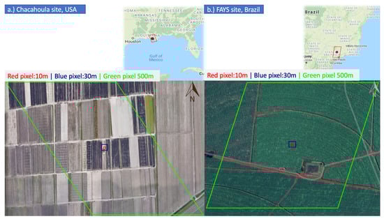
Figure 1.
The two sugarcane locations with EC flux tower sites (red doted polygons; (a) USA and (b) Brazil) displaying the pixel size of the optical data utilized in the study: 10 m (red polygon, Sentinel-2), 30 m (blue polygon, Landsat), and 500 m (green polygon, MODIS).
The Louisiana EC flux tower site (Chacahoula) (29.6341°N, 90.8349°W) had an annual mean temperature of 23.6 °C and an annual precipitation of 1200 mm. The site had Cancienne silty clay loam (Fluvaquentic Epiaquepts) type soil. The fields were graded with a 0.2% slope towards the south, and the elevation of the fields ranged between 2.40 m and 0.61 m over 700–900 m. Sugarcane cultivation in Louisiana dates back to 1850 [78], and the study site had experienced more than 50 years of continuous sugarcane production. The field was cultivated with sugarcane variety HoCP 04-838′, reg. no. CV-181, PI 687221, and the sugarcane plants were spaced at 1.83 m intervals for single-planted rows and 2.44 m for double-planted rows (<1% total field area). Sugarcane crop green up typically occurs in April, while it is harvested between October and December. The EC tower on the site was in a 60 m2 unplanted area surrounded by commercial sugarcane crops. The sugarcane annually received 89 kg ha−1 of nitrogen fertilizer in April.
The Sao Paulo EC flux tower site (FAYS) (21.9506°S, 47.3394°W) had an annual mean temperature of 21.4 °C, annual precipitation of 1410 mm, and gentle slope of <2%. Sugarcane new stem cutting (IAC-5000 variety) was completed on 10/2015 (DOY 275), and the distance between the plotting rows was 1.5 m, with a canopy height of ~5 m during the growing season. The soil type was clay (65% clay, 21% sand, silt 14%), and the site was managed under regular tillage, receiving superphosphate (28% P2O5) and 100 Mg ha−1 dry matter of filter cake (sugar production residue) [31]. The flux tower at this site was installed 24 days after planting. Sugarcane is a multi-year ratoon crop; typically, in Brazil, the crop cycle includes one plant crop and four ratoon crops [30]. The first harvest took place in late October 2016, and the ground trash was left on the soil; nitrogen fertilizer (80 kg N ha−1) and potassium (180 Kg K2O ha−1) were applied two days later [31].
2.2. Weather and CO2 Flux Data for the Sugarcane Plantations
2.2.1. Louisiana, USA Site
The 10 m tower had an integrated open-path infrared gas analyzer, and climate and CO2 flux data outputs were produced at a 30 min temporal resolution (Irgason, Campbell Scientific, Logan, UT, USA). The ecosystem carbon uptake was estimated using the difference between the measured net ecosystem exchange (NEE) and daytime ecosystem respiration (R); daytime and night-time R were calculated based on fitted exponential equations [25,79]. The data covered three growing seasons at the sugarcane plantation (01/2018–12/2020). Multiple sensors at the Chacahoula site were recalibrated in the month of April in 2018 and 2019, resulting in major flags in the CO2 flux data during the subsequent months; for this reason, some of the data were removed from the study.
2.2.2. Sao Paulo, Brazil Site
The tower had an incorporated open-path infrared gas analyzer. Weather and CO2 flux data were obtained at a 30 min temporal resolution, and the height of the tower was 9 m. Gross primary production (GPP) and Ra were calculated at the EC tower based on the NEE observations using the flux-partitioning REddyProc package [80]. The data covered two growing seasons for the Sao Paulo site (October 2015–August 2017).
2.2.3. Pre-Processing of CO2 Flux and Climate Data
GPP at both the sites was estimated from the partitioning of the half-hourly NEE data using the algorithms in [25,26]. The estimated half-hour GPP (GPPEC) and photosynthetically active radiation (PAR) data were recalculated into 1-day and 8-day data using the method presented in [35]. PAR data were estimated as 0.48 of the total incoming short-wave radiation and converted into photosynthetic photon flux density (PPFD) using the approximation 1 W m−2 ≈ 4.57 μmol m−2 s−1 [81].
Air temperature was averaged into daily daytime mean air temperature (TDT) and daily mean air temperature (TDA). We calculated TDT as the average temperature over the half-hour periods that had more than 10 μmol m−2 s−1 PAR within a day. We calculated the 8-day averages of TDT and TDA. There are notable differences between TDA and TDT, and we used TDT for the photosynthesis–temperature relationship in our previous studies [35,49].
2.3. Land Surface Reflectance and Vegetation Index Data
We used the surface reflectance data from MODIS (MOD09A1), Landsat (7 ETM+ and 8 OLI/TIRS), and Sentinel-2/A-2/B, which are accessible on the Google Earth Engine (GEE) platform [82]. For each flux tower site, we selected one MODIS pixel, one Landsat pixel, and one Sentinel-2 pixel centered on the tower coordinates.
The MOD09A1 Collection 6 product [83] provides surface reflectance at a 500 m spatial resolution and 8-day temporal resolution. We employed the Google Earth Engine (GEE) platform [82] to calculate the enhanced vegetation index (EVI) [84] and land surface water index (LSWI) [85] using the surface reflectance data (see Equations (1) and (2)) and assessed the quality of individual observations via the quality band.
EVI = 2.5 × (NIR − Red)/(NIR + 6 × Red−7.5 × Blue + 1)
LSWI = (NIR − SWIR)/(NIR + SWIR)
For Landsat 7 ETM+ and Landsat 8 OLI sensors, atmospherically corrected surface reflectance data at a 30 m spatial resolution were used to calculate the EVI and LSWI. We assessed the individual observations’ data quality using cloud, shadow, water, and snow masks [86]. The blue band was used for an additional quality check by detecting the observations with cloudy and water pixels [87].
Sentinel-2 provides optical data at high spatial resolutions (10 m, 20 m, 60 m) and a 10-day temporal resolution [88]. S2-A (launched June 2015) and S2-B (launched March 2017) have 13 spectral bands, including visible and NIR bands at a 10 m spatial resolution and red-edge and SWIR bands at a 20 m spatial resolution [89]. We used the 10 m S2 orthorectified atmospherically corrected surface reflectance available on GEE. We assessed the quality of individual observations using the cloud bit mask, cirrus bit mask, and blue band [87].
For each eddy flux tower site, the time-series Landsat and Sentinel-2 observations were combined to form one time series of collated data. Both systems provide a 12-bit radiometric resolution with similar reflective wavelengths [88,90,91] and information sensed over the same areas. The similarities between the Landsat and Sentinel-2 spectral resolutions facilitates the combined use of their datasets in several different ways, including data fusion, as reported in previous studies [92]. Landsat and Sentinel-2 were combined without resampling the Landsat 30 m data into 10 m data, since the pixel chosen was within the tower’s footprint and there were no changes in the crop management landcover type within the 30 m Landsat pixel. In our analysis, we integrated various vegetation indices derived from different optical datasets and, in cases where there were observations with overlapping dates, we selected a single observation for each date. This selection was based on the data quality (maximum NDVI), as in past studies [90,92,93]. Ultimately, the gaps in the combined Landsat/Sentinel time-series data were filled in, but the data were not subjected to smoothing. This decision was possible as there was at least one good-quality observation per week, and we ran the model at weekly intervals.
We analyzed the time-series data of the EVI, LSWI, and GPP at the sugarcane sites to identify the start, end, and length of the sugarcane growing season (SOS, EOS, GSL). This information was determined using the VI data with the thresholds of EVI > 0.1 and LSWI > 0 for the SOS and EVI < 0.1 and LSWI < 0 for the EOS. The VI-based GSL was compared with a GPP-based GSL that used SOS > 1 g C m−2 day−1 and EOS < 1 g C m−2 day−1 over three consecutive 8-day periods as thresholds.
2.4. Vegetation Photosynthesis Model (VPM)
The vegetation photosynthesis model (VPM) produces daily estimates of GPP [29]. The VPM calculates the amount of solar energy absorbed by chlorophyll in the canopy (APARchl) and the light use efficiency (LUEg). The EVI is used as a proxy for FPARchl (5).
GPP = APARchl × LUEg
APARchl = FPARchl × PAR
FPARchl = 1.25 × (EVI − 0.1)
LUEg = LUE0 × Tscalar × Wscalar
LUE0 is the apparent quantum yield or maximum light use efficiency (μmol CO2/μmol PPFD), and it has different values for C3 and C4 plants in the VPM. The LUE0 value for C4 plants (e.g., sugarcane) is 0.075 mol of CO2 mol−1 PPFD (0.9 g C mol−1 PPFD) according to earlier works on the vegetation carbon uptake and quantum yield of photosynthesis for sugarcane [35,94]. The LUE0 for C3 plants ranges between 0.42 and 0.65 g CO2 mol−1 PPFD (5.0–7.8 g C mol−1 PPFD) [47,95,96]. The VPM accounts for the presence of C3 and C4 plants in areas that have both by including the fractions of C3 plants (C3F) and C4 plants (C4F).
LUE0 = LUE0-C3 × C3F + LUE0-C4 × C4F
The effects of temperature and water on GPP [49,97] are introduced by Tscalar and Wscalar, respectively. The LSWI is used to calculate Wscalar. Tscalar is based on the Terrestrial Ecosystem Model (TEM) [98].
°T is the air temperature, and Tmin, Topt, and Tmax are the minimum, optimum, and maximum temperatures for photosynthetic activity, respectively. We defined Tmin as −1 °C and Tmax as 48 °C using the same cropland biome parameter values as in [47]. Topt was set as 28 °C, following [35], which estimated Topt from the relationship between the daily average daytime temperature (TDT) and either the GPPEC or vegetation index (EVI).
For comparison, we carried out two sets of VPM simulations to estimate daily GPP using site climate data alongside (1) time-series EVI and LSWI data from Landsat and Sentinel images (GPPVPM-LS) and (2) time-series EVI and LSWI data from MODIS images (GPPVPM-MOD).
2.5. Vegetation Transpiration Model (VTM)
In a crop field, evapotranspiration comprises evaporation (E) from the soil and intercepted canopy water and transpiration (T) from plants [66,99]. During the crop growing season, transpiration usually exceeds evaporation [100,101,102]. At the foliar level, there is a strong linkage between photosynthesis (gross primary production, GPP) and transpiration. This often results in the calculation of the leaf-level water use efficiency as the ratio between these two (i.e., WUELeaf = GPP/T, expressed in mol CO2/mol H2O). The Vegetation Transpiration Model (VTM) predicts daily transpiration as an outcome of GPP and WUELeaf, and it was first tested in grassland ecosystems [103]. Literature data indicate that the WUELeaf_C3 for C3 plants is 500 µmol CO2/µmol H2O, while for C4 plants, the WUELeaf_C4 is 250 µmol CO2/µmol H2O [104].
T = (C3F × 1/WUELeaf_c3 + C4F ∗ 1/WUELeaf_C4) × GPP,
If C3F = 1.0, T (mm H2O/day) = 0.33 (mm H2O/g C/m2/day) × GPP (g C/m2/day)
If C4F = 1.0, T (mm H2O/day) = 0.165 (mm H2O/g C/m2/day) × GPP (g C/m2/day)
2.6. Statistical Analysis
We assessed the biophysical performance of the EVI in terms of GPP changes and seasonal behavior at the sugarcane plantations. We analyzed data from two growing seasons for the Brazil site and three growing seasons for the USA site.
GPPVPM data were assessed with GPPEC data at daily and 8-day scales. In a similar way, the TVTM estimates were compared against the ETEC. In addition, 8-day ET estimates from the MOD16 product were included in the comparison with the ETEC to provide a reference for the performance of one of the most common data products for this variable. The metrics for assessment included the coefficient of determination (R-squared, R2), the Pearson correlation coefficient (p), the mean absolute error (MAE), and the normalized root mean squared error (NRMSE). Finally, we compared the ETEC:P and TVTM:ETEC ratios for the periods with data available to better explore the interannual changes and performance of the model capturing this variability.
3. Results
3.1. Seasonal Dynamics of Climate, Vegetation Indices, and Carbon Fluxes (NEE, GPP)
3.1.1. Seasonal Dynamics of Climate
The Brazil site (Figure 2a) had a tropical climate, characterized by a dry and a wet season, which is typical in tropical regions, with January being the wettest month (247 mm) and July the driest month (27 mm) [30,31]. The annual rainfall was higher during the first crop cycle (1651 mm) than during the second crop cycle (1446 mm). The seasonal dynamics of the daily mean air temperature (TDA) ranged between 14 °C and 26 °C. The mean daily PAR in a year was 39.9 mol m−2 day−1, varying from the lowest in June (19.18 mol m−2 day−1) to the highest in February (55.7 mol m−2 day−1) (Figure 2a).
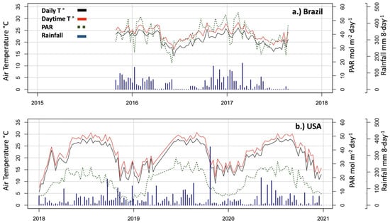
Figure 2.
Seasonal variation in daily temperature, daily mean daytime temperature, 8-day average photosynthetically active radiation (PAR), and accumulated rainfall (8-day interval) of the sugarcane EC flux tower sites. (a) FAYS-Brazil site 2015–2017. (b) Chacahoula, USA site 2018–2020.
The USA site had a sub-tropical climate, characterized by four seasons and a moderately cold winter. On average, March was the driest month (48 mm) and August the wettest month (188 mm) at this site. The second crop cycle was the wettest (1720 mm), and the third cycle was the driest (1477 mm). The air temperature ranged between 5 °C TDA in the winter and 30 °C TDA in the summer. The daily daytime mean air temperature (TDT) was 2–3 degrees higher than the daily mean air temperature (TDA). The average daily PAR in a year was 18.19 (mol m−2 day−1) for the three crop cycles, varying from the lowest in the winter (1.8 mol m−2 day−1 in January) to the highest in the summer (34 mol m−2 day−1 in June) (Figure 2b).
3.1.2. Seasonal Dynamics of Vegetation Indices
At the Brazil site (Figure 3c), the EVI and LSWI rose rapidly in December, reaching the maximum value in May 2015. The EVI and LSWI gradually decreased, and by October the EVI reached below 0.1 and the LSWI below 0. The field was harvested in October 2016. The VI-based start of the sugarcane growing season (SOS) at this site was November 2015 for the first cycle and early December 2016 for the second cycle. The end of the growing season (EOS) was in late October 2016, according to the thresholds used in our previous study [35], which were EVI < 0.1 and LSWI < 0. The results indicated a ~12 month sugarcane growing season length (GSL).
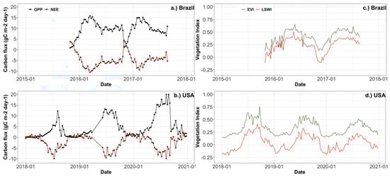
Figure 3.
Seasonal variation in estimated GPPEC and measured NEEEC at 8-day intervals over the study period. Seasonal variation in vegetation indices (land surface water index (LSWI) and enhanced vegetation index (EVI)) derived from 8-day MODIS data. (a,c) FAYS Brazil site, 2015–2017. (b,d) Chacahoula, USA site (2018–2020).
At the USA site (Figure 3d), the EVI and LSWI started to rise in late April and early May and reached their highest values between July and August. The EVI and LSWI gradually dropped, reaching LSWI < 0 and EVI < 0.1 by early November. The VI-based start and end of the sugarcane growing season (SOS and EOS) at this site were May and November, respectively, with a growing season length of 7 months.
3.1.3. Seasonal Dynamics of Carbon Fluxes (NEE and GPP)
At the Brazil site (Figure 3a), the GPPEC rose steadily in November 2015 to higher than 1 g C m−2 day−1, reached the top levels in March, and dropped to 1 g C m−2 day−1 in October 2016. The GPPEC rose again in November 2016, which indicated the start of a new sugarcane growing cycle (Figure 3a). Following the GPP > 1 g C m−2 day−1 criterion, the GPP-based start and end of the growing season (SOS and EOS) at the Brazil site were in November 2015 and October 2016, respectively, which adequately matched the SOS metrics outlined by the vegetation indices (Figure 3a).
At the USA site (Figure 3b), the GPPEC began to increase in late April, was high in the summer, and decreased below 1 g C m−2 day−1 by September in 2018 and November in 2019 and 2020, due to sugarcane harvesting. Following the GPP >= 1 g C m−2 day−1 condition, the GPP-based GSL of sugarcane oscillated between April and November (Figure 3b), which fit sufficiently with the growing season metrics based on the vegetation indices (Figure 3d).
3.2. The Relationships between GPPEC and Vegetation Indices from MODIS, Landsat, and Sentinel-2 Images
For both sugarcane plantations, we assessed in terms of GPP dynamics the biophysical response of the vegetation indices. Figure 4 and Figure 5 show the agreement during the cane growing seasons between the GPPEC and EVI at both plantations.
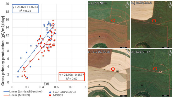
Figure 4.
(Left panel): The relationships between gross primary production (GPPEC) and the enhanced vegetation index (EVI) derived from moderate-spatial-resolution images (MSR, MODIS) and high-spatial-resolution images (HSR, Landsat and Sentinel-2) within the growing season. (Right panel): 3 m 4-band planet Scope and 5 m RapidEye Ortho tile surface reflectance true-color images of vegetation cover in the FAYS Brazil study area. The red circle represents the area used to obtain the time-series of HSR data.
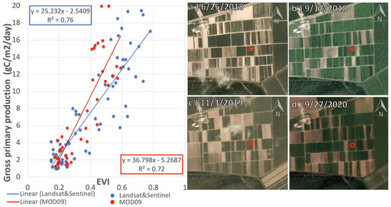
Figure 5.
(Left panel): The relationship between the estimated gross primary production (GPPEC) and enhanced vegetation index derived from moderate-spatial-resolution images (MSR, MODIS) and high-spatial-resolution images (HSR, Landsat and Sentinel-2) within the growing season. (Right panel): 3 m 4-band planet Scope and 5 m RapidEye Ortho tile surface reflectance true-color images of vegetation cover in the Chacahoula, USA study area. The red circle represents the area used to obtain the time-series of HSR data.
At the Brazil site, the GPPEC had a sturdier linear relationship with EVILS-S2 from the Landsat and Sentinel-2 images (R2 = 0.74) than with EVIMODIS from the MODIS image (R2 = 0.67). The difference between Landsat/Sentinel-2 and MODIS can be attributed to the MODIS pixel containing information from neighboring fields with different planting and harvesting dates. Figure 4 illustrates the differences in the crop management of sugarcane fields around the EC site. In February 2016 and August 2016 (Figure 4a,b), within the 500 m MODIS pixel, the south field (February) and the plantation west of the EC tower (August) had bare soil landcover, while the study field had green vegetation. In addition, the effects of radiation changes and cloud cover on the relationship between the GPPEC and the vegetation index are supported by Figure 4d, where green vegetation is visible, but the estimated GPPEC was below 5 g C/m2.
At the USA site, GPPEC also had a stronger correlation with EVILS-S2 (R2 = 0.76) than EVIMODIS (R2 = 0.71) (Figure 5). The sugarcane fields around the EC study field had different planting and harvest dates (Figure 5a–d), which affected the data analysis of the relationship between GPPEC and EVIMOD. Wind conditions influenced the tower’s fetch footprint and varied depending on the season and the landcover type [105,106]. May and June 2018 had high EVI values (0.628) (Figure 3d), and the field was green in June (Figure 5a), but there was no vegetation cover on some of the fallowed sugarcane fields nearby, resulting in a low GPPEC of 3.7 g C/m2. Similar situations were observed on 22 September 2018 (Figure 5b), the date with the highest EVI of 2018 (0.72); October 2019 (Figure 5c); and September 2020 (Figure 5d), for which there were high EVI values (>0.5), relatively low GPPEC values (<5.45 g C/m2), and a harvested field contiguous with the green sugarcane plantation EC site. The sugarcane fields adjacent to the EC site were managed differently and could introduce uncertainty in the MSR data products (i.e., EVIMOD) as some of the fields were within the 500 m MODIS pixel centered on the EC tower.
The slightly lower R2 values at the Brazil site when compared to the USA site were partly attributed to the effect of cloud coverage, increase in shadow during the rainy season, fetch footprint changes throughout the seasons, and influence of the crop management (rotation and harvest) of neighboring sugarcane fields, as evinced by the moderate differences in the vegetation indices (Figure 3a,c).
3.3. Relationships between Air Temperature and GPP and Enhanced Vegetation Index (EVI)
Given the importance of the optimal temperature in multiple biophysical processes and the limited availability of these data, we assessed the relationships between the GPPEC and air temperature (TDT, TDA) during the growing seasons (Figure 6), as this is one of the most reliable methods to estimate Topt. For the site in Brazil, tGPPEC increased as the TDT and TDA rose and reached its plateau at ~25 °C and 23 °C, respectively (Figure 6a,c). In the USA plantation, the GPPEC increased when the TDT and TDA rose and found its plateau at 28 °C and 26 °C, respectively (Figure 6b,d).
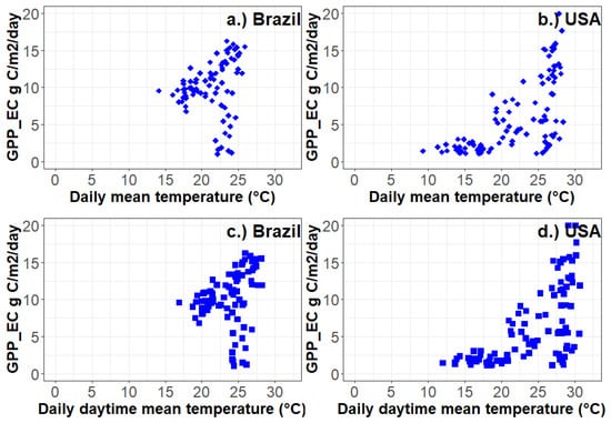
Figure 6.
Relationships between estimated gross primary production (GPP_EC), mean daily temperature, and mean daily daytime temperature within the sugarcane growing seasons. (a,c) FAYS Brazil site, 2015–2017. (b,d) Chacahoula, USA site (2018–2020).
We also studied the relationships between the vegetation index (EVILS-S2, EVIMODIS) and air temperature (TDT and TDA) (Figure 7) as a potential method to calculate Topt. At the Brazil site, both EVILS-S2 and EVIMOD had weak but similar relationships with air temperature (TDT and TDA) (Figure 7a,b). For the TDT, the EVI rose and peaked at 20 °C with a greater density of high values at 26 °C; the EVI reached its plateau at a TDA of 23 °C. The results at the USA location (Figure 7c,d) displayed high EVI values at 28 °C TDT and 25 °C TDA. The results were consistent for both sites and similar for HSR EVILS-S2 and MSR EVIMOD. EVILS-S2 reached a plateau at slightly warmer temperatures at both sites, but remained overall close to the EVIMOD (~0.15 °C). Following these results, the optimum air temperature (Topt) for modeling purposes was established as 25 °C (GPP-based) or 26 °C (EVI-based) for Brazil and 28 °C (GPP-based and EVI-based) for the USA.
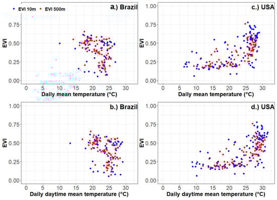
Figure 7.
Relationship between enhanced vegetation index derived from MODIS (EVI 500 m) and Landsat/Sentinel-2 (EVI 10 m) with mean daily air temperature and mean daily daytime temperature during the growing seasons. (a,b) FAYS Brazil site, 2015–2017. (c,d) Chacahoula, USA site (2018–2020).
3.4. Comparison between GPP from VPM Simulations (GPPVPM) and GPP Estimates from the Eddy Flux Sites (GPPEC)
At the Brazil site, the seasonal dynamics of the GPPEC and GPPVPM agreed reasonably well (Figure 8a). The Pearson correlation coefficients and R2 values indicated that there was a stronger relationship between the GPPEC and GPPVPM_LS-S2 (r = 0.86, R2 = 0.74) than between the GPPEC and GPPVPM-MOD (r = 0.78, R2 = 0.62) (Figure 8c, Table 1). The seasonal sums of the GPPEC and GPPVPM within the sugarcane growing season differed noticeably (Table 2).
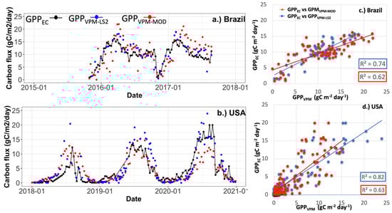
Figure 8.
GPP estimate time series from the EC flux sites (black line) and the VPM (HSR GPP in blue and MSR GPP in red). (a) FAYS Brazil site GPP time series estimates (2015–2017). (b) Chacahoula, USA site GPP time series estimates (2018–2020). Relationship between GPPEC and the VPM (HSR GPP in blue and MSR GPP in red) (c) FAYS Brazil. (d) Chacahoula, USA site.

Table 1.
A comparison of statistical metrics from the correlation analyses between GPPEC (g C m−2 day−1) and GPPVPM (g C m−2 day−1) for the Brazil and USA sites.
Table 2.
Seasonal sums of GPPEC and GPPVPM during the growing the season defined by the GPP-based method and VI-based method at the Brazil and USA sites.
At the USA site, the seasonal dynamics of the GPPEC and GPPVPM agreed reasonably well (Figure 8b). The GPPVPM_LS-S2 values had a stronger relationship with the GPPEC (CC = 0.90, R2 = 0.82) than the GPPVPM-MOD values did with the GPPEC (CC = 0.79, R2 = 0.63) (Figure 8d, Table 1). The seasonal sums of the GPPEC and GPPVPM throughout the growing season also differed noticeably (Table 2).
3.5. Seasonal Dynamics of ET as Measured at the Tower Site (ETEC) and Transpiration as Estimated by VTM Simulations (TVTM)
At the Brazil site, the seasonal dynamics of the ETEC and TVTM_EC agreed reasonably well (Figure 9a). The peak ETEC values ranged between 4 and 5 mm/day during December to February, while the peak TVTM_EC values varied between 2 and 3 mm/day for the same peak periods. The Pearson correlation coefficients and R2 values indicated that there was a moderate relationship between the ETEC and TVTM_EC (p = 0.68, R2 = 0.47) at the Brazil site (Table 3). The Brazil site had the worst performance of the two sites, as the VTM estimates had weak to moderate relationships with the ETEC and TVTM, whereas these relationships at the site in the USA were moderate to strong. The TVTM-LS2 in Brazil (p = 0.45, R2 = 0.21) had a stronger linear relationship than the TVTM-MOD, which had the weakest correlation across the study (p = 0.09, R2 = 0.009). The ETEC/P ratio was consistently ~72.5% in Brazil during the study period, while the TVTM:ETEC ratio for 2016 (complete calendar year) ranged between 64% and 75%, compared to the range of 78% to 95% for 2017 (only including data until August) (Table 4 and Table 5).
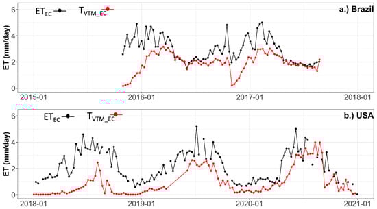
Figure 9.
ETEC estimate time series from the EC flux sites (black line) and the TVTM_EC (red line) for (a) the FAYS Brazil site and (b) Chacahoula, USA.
Table 3.
A comparison of statistical metrics from the correlation analyses between ETEC (mm day−1) and TVTM (mm day−1) for the Brazil and USA sites.
Table 4.
A comparison of the seasonal sums of precipitation, evapotranspiration (ETEC) from the tower observations, and transpiration (TVTM) from the Vegetation Transpiration Model (VTM) simulations. Daily ETEC (mm day−1) and TVTM (mm day−1) from the study sites were aggregated over days with ET observations.
Table 5.
A comparison of the ratio of transpiration (TVTM) to evapotranspiration (ETEC) according to the growing season at the Brazil and USA sites. Daily ETEC (mm day−1) and TVTM (mm day−1) from the study sites were aggregated over days with ET observations for the study period within each year.
The USA site displayed stronger and clearer seasonal dynamics. It had peaks during the summer months, showing ETEC values ranging between 3 and 5 mm/day and TVTM_EC values between 2 and 3 mm/day (2018 and 2019), with higher rates in 2020 ranging between 3 mm/day and 4 mm/day. The year 2020 was the driest year, with an annual total P of 1438 mm, and 2019 was the wettest with a value of 1721 mm. This site displayed the strongest Pearson correlation coefficients and R2 values of either site. For this site, the strongest relationship was between ETEC and TVTM_LS-S2 (p = 0.78, R2 = 0.61), while the relationship between ETEC and TVTM_MOD remained moderate (p = 0.72, R2 = 0.52) (Table 3). Table 4 and Table 5 display the results of the TVTM estimates derived using the GPPEC (TVTM-EC), GPPVPM-LS2 (TVTM-LS2), and GPPVPM-MOD09 (TVTM-MOD09). The ETEC:P ratios had a similar magnitude over the years (45% to 51%), the TVTM:ETEC ratios varied widely, with a 41% average for 2018, 79% average for 2019, and abnormally high average of 91% for 2020.
4. Discussion
4.1. Biophysical Performance of Vegetations Indices from Landsat and Sentinel-2 at Sugarcane Plantations
The one advantage of MODIS sensors (MSR images) is that they acquire images daily and could provide enough good-quality observations to track temporal changes in the vegetation canopy. Many studies have demonstrated that time-series VI data derived from MODIS images at daily and 8-day temporal resolutions can effectively track the seasonal variation and interannual dynamics of vegetation canopies [29,107,108,109,110]. In comparison, as Landsat and Sentinel-2 (HSR images) acquire images at multi-day intervals (for example, Landsat has a 16-day revisit cycle and Sentinel-2 has a 10-day revisit cycle), one sensor often cannot provide enough good-quality observations to track temporal changes in the vegetation canopy. A few studies have combined Landsat images and Sentinel-2 images to construct VI time series and then used them to track the seasonal dynamics of the vegetation canopy [76,111,112,113]. In comparison to the MODIS time-series data, our results also showed that a combination of Landsat and Sentinel-2A/B images increased the number of good-quality observations, providing sufficient data to track the seasonal dynamics and interannual variation of the sugarcane canopy at the Brazil (tropical climate) and USA (subtropical climate) sites. Furthermore, our results indicated that despite the limitations of HSR data in tropical climates, the combined time series of the Landsat and Sentinel-2A/B images provided a better representation of the vegetation carbon uptake, with a linear relationship (R2 = 0.74) stronger than the linear relationship between EVIMODIS and the EC site vegetation carbon uptake data (R2 = 0.67).
One MODIS pixel (MSR, 500 m) often contains multiple crop fields, which could be cultivated with different types of crops or the same type of crop with different management practices, and thus reflects the spectral properties of mixed-crop fields and/or crops under various management practices [114,115,116]. For example, within the MODIS pixel for the USA sugarcane site, there were seven sugarcane fields at different stages in the crop cycle (e.g., fallow, recently planted cane, and ratooning cane) with different management practices, which may have affected the relationship between the MODIS-based VI values and the GPPEC. The results from this study showed that the relationships between the GPPEC and EVI at the sugarcane plantations were stronger when the EVI was calculated from the Landsat/Sentinel-2 (HSR) images than when the EVI was calculated from the MODIS (MSR) images. Other studies have found similar results, highlighting the benefits of high-spatial-resolution images and their contribution to stronger correlations between carbon flux data and vegetation indices on grasslands and croplands [117,118,119]. This is important for estimating crop performance and vegetation health insurance indices over farms with multiple types of crops, rotations, and management techniques [119,120,121].
Sugarcane yields are affected by genotype, environmental conditions, and the time of harvest [122]. Our results showed that the EVI and LSWI tracked the phenological dynamics of sugarcane plantations well, providing a detailed cultivation history for the sugarcane at both plantations [31,77,123]. The LSWI was able to delineate the phenological metrics (SOS, EOS) and identify the harvest dates, consistent with previous studies on sugarcane and other crop types [35,124,125]. As the sugarcane plants at these two sites were harvested while they were still green, the unique phenomenon of the LSWI dropping to <0 reflected the physical system change from green sugarcane fields to brown crop residue and bare soils after harvest at both sites. The harvest date, or EOS, corresponded with the time of the initial negative LSWI value. Our results showed that the harvest dates at the Brazil and USA plantations were accurately recognized by the VI-based algorithms. However, these algorithms had limitations in identifying the SOS at the USA site, which was detected 2 to 4 weeks later across the three growing seasons. These differences could potentially impact the annual total vegetation carbon uptake in the fields. Note that the seasonal changes in GPPEC and NEEEC could also be used to track and delineate the surface phenology of croplands in terms of physiology. The GPPEC accurately tracked the vegetation carbon fixation period using the GPPEC ≥ 1 g C/m2/day criterion. Our results showed that the temporal agreement of the land surface phenology metrics derived from the VI-based and GPPEC-based approaches was stronger for the USA site when the VI values from Landsat/Sentinel-2 (HSR) images were used, in part because the MODIS pixel at the USA site covered several crop fields. Finally, the results agreed well with other studies, like that of Zhang (2022) [76], which highlighted the potential of Landsat/Sentinel-2 images in representing planting patterns over agroecosystems. Finally, this study demonstrated the capabilities and limitations of the VI-based method in determining the growing season length.
4.2. Comparison of GPP Estimates Using Landsat/Sentinel-2 Data and MODIS Data
In comparison to major grain crops (e.g., maize, soybean, winter wheat, and rice), only a few studies have assessed GPP estimates of sugarcane plantations from light use efficiency models with MODIS data [35,47,126]. GPPEC estimates are widely used to assess GPP calculations from light use efficiency models [47,127,128]. In our study analyzing data from 2015–2017 in Brazil and 2018–2020 in the USA, the GPP estimates from the VPM simulations with MODIS images and local climate data agreed reasonably well with the GPPEC data, being consistent with the results reported in Xin et al. 2020 [35], where GPP estimates were evaluated using 2005–2007 data from an eddy flux tower site in Brazil and 2017 data from an eddy flux tower site in USA.
The results of our study showed that the temporal agreement between GPPEC and GPPVPM-LS-S2 (R2 0.82 and 0.74) was stronger than the temporal agreement between GPPEC and GPPVPM-MOD (R2 0.63 and 0.62), which could largely be attributed to two factors: (1) individual MODIS pixels often included multiple crop fields that have different management practices and cultivation calendars (green-up dates and harvest dates), and (2) the footprints of the eddy flux tower sites were much smaller than the MODIS pixels (500 m), corresponding well with the MODIS limitations reported in other studies [129,130,131] investigating the vegetation carbon uptake in crops. In comparison, vegetation indices from Landsat and Sentinel-2 images, which are used to calculate fPARchl and Wscalar, often reflect the vegetation canopy dynamics from one crop field within the footprint of the eddy flux tower site [132,133].
The stronger correlations between EVILS-S2 and GPPEC highlighted in Section 4.1 underscore the influence of vegetation indices on the VPM performance. On the other hand, the EVI values at both an MSR and HSR displayed similar results in estimating the site-specific optimal temperature, which is a crucial parameter to enhance the accuracy of GPP estimates. These results were consistent with other studies, where authors such as Velez (2022) [134] have highlighted the potential of HSR (10 m) vegetation index time series in assessing relevant agronomic parameters. In our study, the EVI was used as opposed to the NDVI given its limitations in canopies, which can become oversaturated, as with sugarcane. The results of our investigation evidenced the potential of the VPM fed with Landsat and Sentinel-2 images for estimating the GPP of sugarcane plantations under different climate zones, sugarcane varieties, and crop practices. Finally, the results underscored the potential of the VPM as a tool for crop growth monitoring in precision agriculture that addresses some of the complexity and scalability issues of typical crop models [135,136].
4.3. Sources of Uncertainties and Errors in VPM Simulations for Sugarcane Plantations
The sources of errors and uncertainties in the GPP estimates from light use efficiency models comprise the model structure; model parameters; and input datasets, including satellite images and climate data. Xin et al. (2020) discussed VPM simulations at two sugarcane sites with a focus on the LUE parameter. The maximum LUE affects the vegetation carbon uptake at the ecosystem level [48,137,138,139] and can be estimated through a linear regression between the aboveground dry biomass and total amount of radiation captured by the vegetation [140,141] or based on the relationship between the PAR and GPP [142]. The LUE values have a large range of variability over sugarcane depending on the climate conditions, altitude, and crop management [142,143,144,145,146]. Our results suggested a maximum LUE ranging between 0.7 and 0.9 g C mol−1 PPFD for Brazil, similar to the ranges reported in other studies in the Brazilian region [147]. Xin et al. (2020) [35] reported that the maximum LUE for VPM simulations was set to 0.9 g C mol−1 PPFD for both sugarcane sites. Further studies are needed to evaluate the maximum LUE parameter over sugarcane plantation sites worldwide, as it could introduce a source of uncertainty for the regional and global GPP estimations.
The comparison of VPM simulations based on MSR images and HSR images illustrates the error sources and uncertainty associated with landcover types within one image pixel and the spatial mismatch (inconsistency) between image pixels and the footprints of an eddy flux tower site [148,149]. One MSR pixel often contains multiple landcover types, often called a mixed pixel, while one HSR pixel most likely contains one landcover type, often called a pure pixel [117,150,151]. The presence of different landcover types within a single pixel affects the model’s representation of the fraction of PAR absorbed by chlorophyll and the vegetation water response, both strong drivers of vegetation carbon uptake. Moreover, the number of good-quality observations from satellite optical sensors would decrease if frequent clouds occurred. In addition, EC flux tower estimates are influenced by the surrounding fields as the footprint changes with the season, weather conditions, vegetation height, and vegetation cover [66,106,148]. The sources of uncertainty from the EC tower increase the challenges of validating GPP estimates, and the sources of error in the system increase based on the condition of the instruments and sensors. In this study, we also used the NEE and latent heat flux data from the tower sties to identify additional poor-quality data in the time series that were not removed by the site’s quality assurance filters.
4.4. Capabilities and limitations of VTM-Forecasted Transpiration for Sugarcane Plantations
The correlation between ETEC and TVTM for the Brazil site was moderate for the TVTM_EC model (R2 = 0.47) but exhibited lower values for TVTM_MOD (R2 = 0.009) and TVTM_LS-S2 (R2 = 0.21), indicating that further improvement and additional variables should be considered in sites located in tropical environments like the Brazil site, where elements such as the residual straw and Bowen ratio variability can affect the transpiration and evapotranspiration rates [152], whereas the more wider spaced rows in Louisiana (1.5 m single row compared to 1.83 m single row and 2.4 m double row) could have affected these water rates [153]. Conversely, the USA site showed a robust correlation across all VTM estimates, especially for the high-spatial-resolution TVTM_LS-S2 (R2 = 0.61), which outperformed the estimates calculated using the GPPEC data as an input for the VTM. The observed differences could be attributed to various factors, including the climatic conditions, soil properties, row spacing, data quality, and sugarcane varieties.
The annual total data in Table 4 underscore the inherent variability in precipitation, ETEC, and TVTM across the sites. Ref. [154] highlighted the changes in actual evaporation and transpiration linked to climate change as one of the leading factors in the interannual yield variability of sugarcane in Brazil. The USA site exhibited the largest interannual variation in precipitation, ETEC, and transpiration VTM rates. Ref. [155] emphasized the impact of soil water conditions as the main driver of the interannual variability in ET and T, partially explaining some the differences observed in the TVTM:ETEC ratios over time. Moreover, ref. [156] addressed the significance of row spacing, as it increases soil water content and provides more space for the sugarcane to grow, significantly increasing transpiration in periods of low rainfall, which could partially explain some of the abnormally high TVTM rates at the USA site in 2020 (driest year). In addition, some of the differences between the MSR and HSR transpiration estimates can be linked to the fact that the MSR pixel included multiple fields containing different varieties and, in some cases, different management practices.
The VTM showed a strong capacity to capture the seasonal dynamics and some of the interannual variability in the transpiration rates. Despite the simplicity of the approach, overall, the TVTM results captured the seasonal dynamics of the water flux, underscoring the potential of this tool and its applications. However, the variability across different scales in the results suggests that for field-level and commercial applications the time-scale dependency should be further studied, and additional parameters such as initial water content and row spacing should be included to provide a better field representation of the transpiration water flux.
5. Conclusions
This study successfully explored the use of Landsat and Sentinel-2 imagery to monitor phenology and as an input for gross primary production (GPP) estimation in sugarcane plantations in São Paulo, Brazil, and Louisiana, USA. Our findings contribute significantly to the field of remote sensing in agriculture, offering new perspectives and methodologies. The key conclusions and contributions include:
- Potential of Landsat and Sentinel-2 over cloudy environments: We demonstrated the effective combination of Landsat and Sentinel-2 time-series images for monitoring phenology and as an input for GPP estimation in sugarcane plantations. This approach proved particularly effective in diverse environmental conditions, including cloudy scenarios where HSR images have the greatest limitations, thereby underscoring the robustness of these satellite images in capturing agricultural dynamics. Furthermore, HSR data better represented field vegetation carbon uptake at both sites compared to MSR data.
- EVI as a proxy for estimating optimal air temperature: The study revealed a novel application of the enhanced vegetation index (EVI) in estimating site-specific optimal air temperature (Topt) for photosynthesis. This correlation between the GPPEC, EVI, and air temperature variables opens up new avenues for understanding the biophysical performance of vegetation indices across different pixels and fields.
- VPM efficacy: Our research highlighted the VPM’s capabilities for accurately estimating the seasonal dynamics of GPP in sugarcane plantations at a high spatial resolution. The model’s adaptability to varying environmental conditions was a key finding, showcasing its potential for broader application. Nonetheless, the field variability of the ECT footprint introduced some uncertainty into the ground data.
- Transpiration modeling insights: The Vegetation Transpiration Model (VTM) effectively captured the seasonal dynamics of transpiration. However, its dependency on high-quality GPP data and the need for further research into time-scale dependency and initial water content impact were noted. The model showed promise in environments like Louisiana, but additional research is needed in settings like Brazil to refine its accuracy and address uncertainties.
Future work will include assessments of the models at additional sugarcane plantations with EC flux systems, spatial yield data, and detailed field information including variety type and row spacing, as this could increase our knowledge regarding likely sources of uncertainty and the prospects of deploying the models as tools for precision agriculture.
Author Contributions
The authors J.C. and X.X. were responsible for the conceptualization, methodology, and outline design, with J.C. also handling the outline design, modeling, and analysis. P.M.W.J. managed the software aspect of the Louisiana sugarcane EC data processing, while O.M.R.C. and H.C.F. handled the software for processing the EC data from Brazil. All authors contributed to the discussion and identifying current knowledge gaps. Validation was conducted by J.C. and reviewed by X.X., P.M.W.J. and O.M.R.C. All authors provided significant feedback on the review of the manuscript and editing. All authors have read and agreed to the published version of the manuscript.
Funding
This study was supported by the USDA National Institute of Food and Agriculture (grant 2020-67104-30935) and NASA GeoCarb Mission (GeoCarb contract No. 80LARC17C0001). The site in Brazil was funded by FAPESP (2014/24452-0) and Embrapa Meio Ambiente (03.15.00.117).
Data Availability Statement
Optical satellite data were obtained and are available from Google Earth Engine. EC data can be requested from the site administrators or the authors of this manuscript. Any additional data produced herein can be requested from the authors of this document.
Acknowledgments
We thank the reviewers for their time and effort in reviewing the manuscript, as their comments and suggestions helped us to further improve this manuscript.
Conflicts of Interest
The authors declare no conflict of interest.
References
- Goldemberg, J.; Coelho, S.T.; Guardabassi, P. The sustainability of ethanol production from sugarcane. Energy Policy 2008, 36, 2086–2097. [Google Scholar] [CrossRef]
- Demirbas, A. Biofuels securing the planet’s future energy needs. Energy Convers. Manag. 2009, 50, 2239–2249. [Google Scholar] [CrossRef]
- Lakshmanan, P.; Geijskes, R.J.; Aitken, K.S.; Grof, C.L.P.; Bonnett, G.D.; Smith, G.R. Sugarcane biotechnology: The challenges and opportunities. Vitro Cell. Dev. Biol.-Plant 2005, 41, 345–363. [Google Scholar] [CrossRef]
- Yadav, S.; Jackson, P.; Wei, X.; Ross, E.M.; Aitken, K.; Deomano, E.; Atkin, F.; Hayes, B.J.; Voss-Fels, K.P. Accelerating genetic gain in sugarcane breeding using genomic selection. Agronomy 2020, 10, 585. [Google Scholar] [CrossRef]
- de Matos, M.; Santos, F.; Eichler, P. Sugarcane world scenario. In Sugarcane Biorefinery, Technology and Perspectives; Elsevier: Amsterdam, The Netherlands, 2020; pp. 1–19. [Google Scholar]
- FAO. United Nations, World Food and Agriculture—Statistical Yearbook 2020; FAO: Rome, Italy, 2020; ISBN 978-92-5-133394-5. [Google Scholar]
- Tracking Clean Energy Progress—Topics. Available online: https://www.iea.org/topics/tracking-clean-energy-progress (accessed on 21 October 2021).
- dos Santos Simões, M.; Rocha, J.V.; Lamparelli, R.A.C. Spectral variables, growth analysis and yield of sugarcane. Sci. Agric. 2005, 62, 199–207. [Google Scholar] [CrossRef]
- Campbell, J.E.; Berry, J.A.; Seibt, U.; Smith, S.J.; Montzka, S.A.; Launois, T.; Belviso, S.; Bopp, L.; Laine, M. Large historical growth in global terrestrial gross primary production. Nature 2017, 544, 84–87. [Google Scholar] [CrossRef] [PubMed]
- Amthor, J.S. Terrestrial higher-plant response to increasing atmospheric [CO2] in relation to the global carbon cycle. Glob. Change Biol. 1995, 1, 243–274. [Google Scholar] [CrossRef]
- Beer, C.; Reichstein, M.; Tomelleri, E.; Ciais, P.; Jung, M.; Carvalhais, N.; Rödenbeck, C.; Arain, M.A.; Baldocchi, D.; Bonan, G.B. Terrestrial gross carbon dioxide uptake: Global distribution and covariation with climate. Science 2010, 329, 834–838. [Google Scholar] [CrossRef]
- Lambers, H.; Chapin, F.S., III; Pons, T.L. Plant Physiological Ecology; Springer Science & Business Media: New York, NY, USA, 2008. [Google Scholar]
- Sitch, S.; Smith, B.; Prentice, I.C.; Arneth, A.; Bondeau, A.; Cramer, W.; Kaplan, J.O.; Levis, S.; Lucht, W.; Sykes, M.T. Evaluation of ecosystem dynamics, plant geography and terrestrial carbon cycling in the LPJ dynamic global vegetation model. Glob. Change Biol. 2003, 9, 161–185. [Google Scholar] [CrossRef]
- Bondeau, A.; Smith, P.C.; Zaehle, S.; Schaphoff, S.; Lucht, W.; Cramer, W.; Gerten, D.; Lotze-Campen, H.; Müller, C.; Reichstein, M. Modelling the role of agriculture for the 20th century global terrestrial carbon balance. Glob. Change Biol. 2007, 13, 679–706. [Google Scholar] [CrossRef]
- Foley, J.A.; Prentice, I.C.; Ramankutty, N.; Levis, S.; Pollard, D.; Sitch, S.; Haxeltine, A. An integrated biosphere model of land surface processes, terrestrial carbon balance, and vegetation dynamics. Glob. Biogeochem. Cycles 1996, 10, 603–628. [Google Scholar] [CrossRef]
- Zhao, M.; Running, S.W. Drought-Induced Reduction in Global Terrestrial Net Primary Production from 2000 Through 2009. Science 2010, 329, 940–943. [Google Scholar] [CrossRef] [PubMed]
- Doughty, R.; Xiao, X.; Wu, X.; Zhang, Y.; Bajgain, R.; Zhou, Y.; Qin, Y.; Zou, Z.; McCarthy, H.; Friedman, J.; et al. Responses of gross primary production of grasslands and croplands under drought, pluvial, and irrigation conditions during 2010–2016, Oklahoma, USA. Agric. Water Manag. 2018, 204, 47–59. [Google Scholar] [CrossRef]
- He, M.; Kimball, J.S.; Maneta, M.P.; Maxwell, B.D.; Moreno, A.; Beguería, S.; Wu, X. Regional Crop Gross Primary Productivity and Yield Estimation Using Fused Landsat-MODIS Data. Remote Sens. 2018, 10, 372. [Google Scholar] [CrossRef]
- Wu, X.; Xiao, X.; Yang, Z.; Wang, J.; Steiner, J.; Bajgain, R. Spatial-temporal dynamics of maize and soybean planted area, harvested area, gross primary production, and grain production in the Contiguous United States during 2008–2018. Agric. For. Meteorol. 2020, 297, 108240. [Google Scholar] [CrossRef]
- Anav, A.; Friedlingstein, P.; Beer, C.; Ciais, P.; Harper, A.; Jones, C.; Murray-Tortarolo, G.; Papale, D.; Parazoo, N.C.; Peylin, P. Spatiotemporal patterns of terrestrial gross primary production: A review. Rev. Geophys. 2015, 53, 785–818. [Google Scholar] [CrossRef]
- Ma, J.; Yan, X.; Dong, W.; Chou, J. Gross primary production of global forest ecosystems has been overestimated. Sci. Rep. 2015, 5, 10820. [Google Scholar] [CrossRef]
- Papale, D.; Reichstein, M.; Aubinet, M.; Canfora, E.; Bernhofer, C.; Kutsch, W.; Longdoz, B.; Rambal, S.; Valentini, R.; Vesala, T. Towards a standardized processing of Net Ecosystem Exchange measured with eddy covariance technique: Algorithms and uncertainty estimation. Biogeosciences 2006, 3, 571–583. [Google Scholar] [CrossRef]
- Bhattacharyya, P.; Neogi, S.; Roy, K.S.; Rao, K.S. Gross primary production, ecosystem respiration and net ecosystem exchange in Asian rice paddy: An eddy covariance-based approach. Curr. Sci. 2013, 104, 67–75. [Google Scholar]
- Verlinden, M.S.; Broeckx, L.S.; Zona, D.; Berhongaray, G.; De Groote, T.; Camino Serrano, M.; Janssens, I.A.; Ceulemans, R. Net ecosystem production and carbon balance of an SRC poplar plantation during its first rotation. Biomass Bioenergy 2013, 56, 412–422. [Google Scholar] [CrossRef]
- Reichstein, M.; Falge, E.; Baldocchi, D.; Papale, D.; Aubinet, M.; Berbigier, P.; Bernhofer, C.; Buchmann, N.; Gilmanov, T.; Granier, A. On the separation of net ecosystem exchange into assimilation and ecosystem respiration: Review and improved algorithm. Glob. Change Biol. 2005, 11, 1424–1439. [Google Scholar] [CrossRef]
- Reichstein, M.; Bahn, M.; Ciais, P.; Frank, D.; Mahecha, M.D.; Seneviratne, S.I.; Zscheischler, J.; Beer, C.; Buchmann, N.; Frank, D.C.; et al. Climate extremes and the carbon cycle. Nature 2013, 500, 287–295. [Google Scholar] [CrossRef] [PubMed]
- Jung, M.; Reichstein, M.; Bondeau, A. Towards global empirical upscaling of FLUXNET eddy covariance observations: Validation of a model tree ensemble approach using a biosphere model. Biogeosciences 2009, 6, 2001–2013. [Google Scholar] [CrossRef]
- Running, S.W.; Baldocchi, D.D.; Turner, D.P.; Gower, S.T.; Bakwin, P.S.; Hibbard, K.A. A global terrestrial monitoring network integrating tower fluxes, flask sampling, ecosystem modeling and EOS satellite data. Remote Sens. Environ. 1999, 70, 108–127. [Google Scholar] [CrossRef]
- Xiao, X.; Hollinger, D.; Aber, J.; Goltz, M.; Davidson, E.A.; Zhang, Q.; Moore, B., III. Satellite-based modeling of gross primary production in an evergreen needleleaf forest. Remote Sens. Environ. 2004, 89, 519–534. [Google Scholar] [CrossRef]
- Cabral, O.M.; Rocha, H.R.; Gash, J.H.; Ligo, M.A.; Ramos, N.P.; Packer, A.P.; Batista, E.R. Fluxes of CO2 above a sugarcane plantation in Brazil. Agric. For. Meteorol. 2013, 182, 54–66. [Google Scholar] [CrossRef]
- Cabral, O.M.; Freitas, H.C.; Cuadra, S.V.; de Andrade, C.A.; Ramos, N.P.; Grutzmacher, P.; Galdos, M.; Packer, A.P.C.; da Rocha, H.R.; Rossi, P. The sustainability of a sugarcane plantation in Brazil assessed by the eddy covariance fluxes of greenhouse gases. Agric. For. Meteorol. 2020, 282, 107864. [Google Scholar] [CrossRef]
- Flack-Prain, S.; Shi, L.; Zhu, P.; da Rocha, H.R.; Cabral, O.; Hu, S.; Williams, M. The impact of climate change and climate extremes on sugarcane production. GCB Bioenergy 2021, 13, 408–424. [Google Scholar] [CrossRef]
- Pakoktom, T.; Chaichana, N.; Phattaralerphong, J.; Sathornkich, J. Carbon use efficiency of the first ratoon cane by Eddy Covariance Technique. Int. J. Environ. Sci. Dev. 2013, 4, 488–491. [Google Scholar] [CrossRef]
- Ruhoff, A.L.; Paz, A.R.; Aragao, L.; Mu, Q.; Malhi, Y.; Collischonn, W.; Rocha, H.R.; Running, S.W. Assessment of the MODIS global evapotranspiration algorithm using eddy covariance measurements and hydrological modelling in the Rio Grande basin. Hydrol. Sci. J. 2013, 58, 1658–1676. [Google Scholar] [CrossRef]
- Xin, F.; Xiao, X.; Cabral, O.M.; White, P.M.; Guo, H.; Ma, J.; Li, B.; Zhao, B. Understanding the Land Surface Phenology and Gross Primary Production of Sugarcane Plantations by Eddy Flux Measurements, MODIS Images, and Data-Driven Models. Remote Sens. 2020, 12, 2186. [Google Scholar] [CrossRef]
- Clevers, J.; Büker, C.; Van Leeuwen, H.J.C.; Bouman, B.A.M. A framework for monitoring crop growth by combining directional and spectral remote sensing information. Remote Sens. Environ. 1994, 50, 161–170. [Google Scholar] [CrossRef]
- Clevers, J.; Van Leeuwen, H.J.C. Combined use of optical and microwave remote sensing data for crop growth monitoring. Remote Sens. Environ. 1996, 56, 42–51. [Google Scholar] [CrossRef]
- Doraiswamy, P.C.; Moulin, S.; Cook, P.W.; Stern, A. Crop yield assessment from remote sensing. Photogramm. Eng. Remote Sens. 2003, 69, 665–674. [Google Scholar] [CrossRef]
- Moon, M.; Zhang, X.; Henebry, G.M.; Liu, L.; Gray, J.M.; Melaas, E.K.; Friedl, M.A. Long-term continuity in land surface phenology measurements: A comparative assessment of the MODIS land cover dynamics and VIIRS land surface phenology products. Remote Sens. Environ. 2019, 226, 74–92. [Google Scholar] [CrossRef]
- Lees, K.J.; Quaife, T.; Artz, R.R.E.; Khomik, M.; Clark, J.M. Potential for using remote sensing to estimate carbon fluxes across northern peatlands—A review. Sci. Total Environ. 2018, 615, 857–874. [Google Scholar] [CrossRef] [PubMed]
- Wang, J.; Liu, J.; Cao, M.; Liu, Y.; Yu, G.; Li, G.; Qi, S.; Li, K. Modelling carbon fluxes of different forests by coupling a remote-sensing model with an ecosystem process model. Int. J. Remote Sens. 2011, 32, 6539–6567. [Google Scholar] [CrossRef]
- Xiao, J.; Chevallier, F.; Gomez, C.; Guanter, L.; Hicke, J.A.; Huete, A.R.; Ichii, K.; Ni, W.; Pang, Y.; Rahman, A.F.; et al. Remote sensing of the terrestrial carbon cycle: A review of advances over 50 years. Remote Sens. Environ. 2019, 233, 111383. [Google Scholar] [CrossRef]
- Monteith, J.L. Solar radiation and productivity in tropical ecosystems. J. Appl. Ecol. 1972, 9, 747–766. [Google Scholar] [CrossRef]
- Monteith, J.L. Climate and the efficiency of crop production in Britain. Philos. Trans. R. Soc. Lond. B Biol. Sci. 1977, 281, 277–294. [Google Scholar]
- Hilker, T.; Coops, N.C.; Wulder, M.A.; Black, T.A.; Guy, R.D. The use of remote sensing in light use efficiency based models of gross primary production: A review of current status and future requirements. Sci. Total Environ. 2008, 404, 411–423. [Google Scholar] [CrossRef] [PubMed]
- Seaquist, J.W.; Olsson, L.; Ardö, J. A remote sensing-based primary production model for grassland biomes. Ecol. Model. 2003, 169, 131–155. [Google Scholar] [CrossRef]
- Zhang, Y.; Xiao, X.; Wu, X.; Zhou, S.; Zhang, G.; Qin, Y.; Dong, J. A global moderate resolution dataset of gross primary production of vegetation for 2000–2016. Sci. Data 2017, 4, 170165. [Google Scholar] [CrossRef] [PubMed]
- Xiao, X. Light absorption by leaf chlorophyll and maximum light use efficiency. IEEE Trans. Geosci. Remote Sens. 2006, 44, 1933–1935. [Google Scholar] [CrossRef]
- Chang, Q.; Xiao, X.; Doughty, R.; Wu, X.; Jiao, W.; Qin, Y. Assessing variability of optimum air temperature for photosynthesis across site-years, sites and biomes and their effects on photosynthesis estimation. Agric. For. Meteorol. 2021, 298–299, 108277. [Google Scholar] [CrossRef]
- Wu, X.; Xiao, X.; Zhang, Y.; He, W.; Wolf, S.; Chen, J.; He, M.; Gough, C.M.; Qin, Y.; Zhou, Y. Spatiotemporal consistency of four gross primary production products and solar-induced chlorophyll fluorescence in response to climate extremes across CONUS in 2012. J. Geophys. Res. Biogeosci. 2018, 123, 3140–3161. [Google Scholar] [CrossRef]
- Singh, D. Generation and evaluation of gross primary productivity using Landsat data through blending with MODIS data. Int. J. Appl. Earth Obs. Geoinf. 2011, 13, 59–69. [Google Scholar] [CrossRef]
- Running, S.; Mu, Q.; Zhao, M. MOD17A2H MODIS/terra gross primary productivity 8-day L4 global 500m SIN grid V006. NASA EOSDIS Land Process. DAAC 2015, 1–28. [Google Scholar]
- USDA ERS. Farming and Farm Income. Available online: https://www.ers.usda.gov/data-products/ag-and-food-statistics-charting-the-essentials/farming-and-farm-income/ (accessed on 29 January 2021).
- Cerri, C.C.; Galdos, M.V.; Maia, S.M.F.; Bernoux, M.; Feigl, B.J.; Powlson, D.; Cerri, C.E.P. Effect of sugarcane harvesting systems on soil carbon stocks in Brazil: An examination of existing data. Eur. J. Soil Sci. 2011, 62, 23–28. [Google Scholar] [CrossRef]
- de Oliveira Bordonal, R.; de Figueiredo, E.B.; La Scala, N., Jr. Greenhouse gas balance due to the conversion of sugarcane areas from burned to green harvest, considering other conservationist management practices. GCB Bioenergy 2012, 4, 846–858. [Google Scholar] [CrossRef]
- Galdos, M.V.; Cerri, C.C.; Lal, R.; Bernoux, M.; Feigl, B.; Cerri, C.E.P. Net greenhouse gas fluxes in Brazilian ethanol production systems. GCB Bioenergy 2010, 2, 37–44. [Google Scholar] [CrossRef]
- Alkimim, A.; Clarke, K.C. Land use change and the carbon debt for sugarcane ethanol production in Brazil. Land Use Policy 2018, 72, 65–73. [Google Scholar] [CrossRef]
- Khan, I.; Javed, T.; Khan, A.; Lei, H.; Muhammad, I.; Ali, I.; Huo, X. Impact assessment of land use change on surface temperature and agricultural productivity in Peshawar-Pakistan. Environ. Sci. Pollut. Res. 2019, 26, 33076–33085. [Google Scholar] [CrossRef] [PubMed]
- Ai, Z.; Wang, Q.; Yang, Y.; Manevski, K.; Yi, S.; Zhao, X. Variation of gross primary production, evapotranspiration and water use efficiency for global croplands. Agric. For. Meteorol. 2020, 287, 107935. [Google Scholar] [CrossRef]
- Kandasamy, S.; Frederic, B.; Verger, A.; Neveux, P.; Weiss, M. A comparison of methods for smoothing and gap filling time series of remote sensing observations: Application to MODIS LAI products. Biogeosciences 2013, 10, 4055–4071. [Google Scholar] [CrossRef]
- Celis, J.; Xiao, X.; Basara, J.; Wagle, P.; McCarthy, H. Simple and Innovative Methods to Estimate Gross Primary Production and Transpiration of Crops: A Review. In Digital Ecosystem for Innovation in Agriculture; Springer: Singapore, 2023; pp. 125–156. [Google Scholar]
- Allen, R.G.; Tasumi, M.; Trezza, R. Satellite-based energy balance for mapping evapotranspiration with internalized calibration (METRIC)—Model. J. Irrig. Drain. Eng. 2007, 133, 380–394. [Google Scholar] [CrossRef]
- Kool, D.; Agam, N.; Lazarovitch, N.; Heitman, J.L.; Sauer, T.J.; Ben-Gal, A. A review of approaches for evapotranspiration partitioning. Agric. For. Meteorol. 2014, 184, 56–70. [Google Scholar] [CrossRef]
- Monteith, J.L. Evaporation and environment. In Symposia of the Society for Experimental Biology; Cambridge University Press (CUP): Cambridge, UK, 1965; Volume 19, pp. 205–234. [Google Scholar]
- Penman, H.L. Natural evaporation from open water, bare soil and grass. Proc. R. Soc. Lond. Ser. Math. Phys. Sci. 1948, 193, 120–145. [Google Scholar]
- Celis, J.A.; Moreno, H.A.; Basara, J.B.; McPherson, R.A.; Cosh, M.; Ochsner, T.; Xiao, X. From Standard Weather Stations to Virtual Micro-Meteorological Towers in Ungauged Sites: Modeling Tool for Surface Energy Fluxes, Evapotranspiration, Soil Temperature, and Soil Moisture Estimations. Remote Sens. 2021, 13, 1271. [Google Scholar] [CrossRef]
- Ivanov, V.Y.; Vivoni, E.R.; Bras, R.L.; Entekhabi, D. Catchment hydrologic response with a fully distributed triangulated irregular network model. Water Resour. Res. 2004, 40, 11. [Google Scholar] [CrossRef]
- Matsui, T.; Lakshmi, V.; Small, E.E. The effects of satellite-derived vegetation cover variability on simulated land–atmosphere interactions in the NAMS. J. Clim. 2005, 18, 21–40. [Google Scholar] [CrossRef]
- Mu, Q.; Zhao, M.; Running, S.W. Improvements to a MODIS global terrestrial evapotranspiration algorithm. Remote Sens. Environ. 2011, 115, 1781–1800. [Google Scholar] [CrossRef]
- de Arruda Souza, V.; Roberti, D.R.; Ruhoff, A.L.; Zimmer, T.; Adamatti, D.S.; de Gonçalves, L.G.G.; Diaz, M.B.; Alves, R.d.C.M.; de Moraes, O.L. Evaluation of MOD16 algorithm over irrigated rice paddy using flux tower measurements in Southern Brazil. Water 2019, 11, 1911. [Google Scholar] [CrossRef]
- Velpuri, N.M.; Senay, G.B.; Singh, R.K.; Bohms, S.; Verdin, J.P. A comprehensive evaluation of two MODIS evapotranspiration products over the conterminous United States: Using point and gridded FLUXNET and water balance ET. Remote Sens. Environ. 2013, 139, 35–49. [Google Scholar] [CrossRef]
- Meerdink, S.K.; Hook, S.J.; Roberts, D.A.; Abbott, E.A. The ECOSTRESS spectral library version 1.0. Remote Sens. Environ. 2019, 230, 111196. [Google Scholar] [CrossRef]
- Hulley, G.C.; Göttsche, F.M.; Rivera, G.; Hook, S.J.; Freepartner, R.J.; Martin, M.A.; Cawse-Nicholson, K.; Johnson, W.R. Validation and Quality Assessment of the ECOSTRESS Level-2 Land Surface Temperature and Emissivity Product. IEEE Trans. Geosci. Remote Sens. 2022, 60, 1–23. [Google Scholar] [CrossRef]
- Liang, L.; Feng, Y.; Wu, J.; He, X.; Liang, S.; Jiang, X.; de Oliveira, G.; Qiu, J.; Zeng, Z. Evaluation of ECOSTRESS evapotranspiration estimates over heterogeneous landscapes in the continental US. J. Hydrol. 2022, 613, 128470. [Google Scholar] [CrossRef]
- Liu, N.; Oishi, A.C.; Miniat, C.F.; Bolstad, P. An evaluation of ECOSTRESS products of a temperate montane humid forest in a complex terrain environment. Remote Sens. Environ. 2021, 265, 112662. [Google Scholar] [CrossRef]
- Zhang, X.; Xiao, X.; Qiu, S.; Xu, X.; Wang, X.; Chang, Q.; Wu, J.; Li, B. Quantifying latitudinal variation in land surface phenology of Spartina alterniflora saltmarshes across coastal wetlands in China by Landsat 7/8 and Sentinel-2 images. Remote Sens. Environ. 2022, 269, 112810. [Google Scholar] [CrossRef]
- White, P.M.; Webber, C.L.; Viator, R.P.; Aita, G. Sugarcane Biomass, Dry Matter, and Sucrose Availability and Variability When Grown on a Bioenergy Feedstock Production Cycle. BioEnergy Res. 2019, 12, 55–67. [Google Scholar] [CrossRef]
- Hilliard, S.B. Site Characteristics and Spatial Stability of the Louisiana Sugarcane Industry. Agric. Hist. 1979, 53, 254–269. [Google Scholar]
- Reichstein, M.; Tenhunen, J.D.; Roupsard, O.; Ourcival, J.-M.; Rambal, S.; Dore, S.; Valentini, R. Ecosystem respiration in two Mediterranean evergreen Holm Oak forests: Drought effects and decomposition dynamics. Funct. Ecol. 2002, 16, 27–39. [Google Scholar] [CrossRef]
- Wutzler, T.; Lucas-Moffat, A.; Migliavacca, M.; Knauer, J.; Sickel, K.; Šigut, L.; Menzer, O.; Reichstein, M. Basic and extensible post-processing of eddy covariance flux data with REddyProc. Biogeosciences 2018, 15, 5015–5030. [Google Scholar] [CrossRef]
- Thimijan, R.W.; Heins, R.D. Photometric, radiometric, and quantum light units of measure: A review of procedures for interconversion. HortScience 1983, 18, 818–822. [Google Scholar] [CrossRef]
- Gorelick, N.; Hancher, M.; Dixon, M.; Ilyushchenko, S.; Thau, D.; Moore, R. Google Earth Engine: Planetary-scale geospatial analysis for everyone. Remote Sens. Environ. 2017, 202, 18–27. [Google Scholar] [CrossRef]
- Vermote, P.E.F.; Roger, J.C.; Ray, J.P. MODIS Land Surface Reflectance Science Computing Facility Principal Investigator: Dr. Eric F. Vermote Web Site. 2015, p. 35. Available online: http://modis-sr.ltdri.org (accessed on 20 November 2021).
- Huete, A.R.; Liu, H.Q.; Batchily, K.; van Leeuwen, W. A comparison of vegetation indices over a global set of TM images for EOS-MODIS. Remote Sens. Environ. 1997, 59, 440–451. [Google Scholar] [CrossRef]
- Xiao, X.; Zhang, Q.; Braswell, B.; Urbanski, S.; Boles, S.; Wofsy, S.; Moore, B., III; Ojima, D. Modeling gross primary production of temperate deciduous broadleaf forest using satellite images and climate data. Remote Sens. Environ. 2004, 91, 256–270. [Google Scholar] [CrossRef]
- Foga, S.; Scaramuzza, P.L.; Guo, S.; Zhu, Z.; Dilley, R.D., Jr.; Beckmann, T.; Schmidt, G.L.; Dwyer, J.L.; Hughes, M.J.; Laue, B. Cloud detection algorithm comparison and validation for operational Landsat data products. Remote Sens. Environ. 2017, 194, 379–390. [Google Scholar] [CrossRef]
- Du, Y.; Teillet, P.M.; Cihlar, J. Radiometric normalization of multitemporal high-resolution satellite images with quality control for land cover change detection. Remote Sens. Environ. 2002, 82, 123–134. [Google Scholar] [CrossRef]
- Drusch, M.; Del Bello, U.; Carlier, S.; Colin, O.; Fernandez, V.; Gascon, F.; Hoersch, B.; Isola, C.; Laberinti, P.; Martimort, P. Sentinel-2: ESA’s optical high-resolution mission for GMES operational services. Remote Sens. Environ. 2012, 120, 25–36. [Google Scholar] [CrossRef]
- Storey, J.; Roy, D.P.; Masek, J.; Gascon, F.; Dwyer, J.; Choate, M. A note on the temporary misregistration of Landsat-8 Operational Land Imager (OLI) and Sentinel-2 Multi Spectral Instrument (MSI) imagery. Remote Sens. Environ. 2016, 186, 121–122. [Google Scholar] [CrossRef]
- Gascon, F.; Bouzinac, C.; Thépaut, O.; Jung, M.; Francesconi, B.; Louis, J.; Lonjou, V.; Lafrance, B.; Massera, S.; Gaudel-Vacaresse, A.; et al. Copernicus Sentinel-2A Calibration and Products Validation Status. Remote Sens. 2017, 9, 584. [Google Scholar] [CrossRef]
- Irons, J.R.; Dwyer, J.L.; Barsi, J.A. The next Landsat satellite: The Landsat Data Continuity Mission. Remote Sens. Environ. 2012, 122, 11–21. [Google Scholar] [CrossRef]
- Zhang, H.K.; Roy, D.P.; Yan, L.; Li, Z.; Huang, H.; Vermote, E.; Skakun, S.; Roger, J.-C. Characterization of Sentinel-2A and Landsat-8 top of atmosphere, surface, and nadir BRDF adjusted reflectance and NDVI differences. Remote Sens. Environ. 2018, 215, 482–494. [Google Scholar] [CrossRef]
- Markham, B.; Barsi, J.; Kvaran, G.; Ong, L.; Kaita, E.; Biggar, S.; Czapla-Myers, J.; Mishra, N.; Helder, D. Landsat-8 operational land imager radiometric calibration and stability. Remote Sens. 2014, 6, 12275–12308. [Google Scholar] [CrossRef]
- Meinzer, F.C.; Zhu, J. Nitrogen stress reduces the efficiency of the C4CO2 concentrating system, and therefore quantum yield, in Saccharum (sugarcane) species. J. Exp. Bot. 1998, 49, 1227–1234. [Google Scholar] [CrossRef]
- Ma, J.; Xiao, X.; Zhang, Y.; Doughty, R.; Chen, B.; Zhao, B. Spatial-temporal consistency between gross primary productivity and solar-induced chlorophyll fluorescence of vegetation in China during 2007–2014. Sci. Total Environ. 2018, 639, 1241–1253. [Google Scholar] [CrossRef]
- Yuan, W.; Liu, S.; Zhou, G.; Zhou, G.; Tieszen, L.L.; Baldocchi, D.; Bernhofer, C.; Gholz, H.; Goldstein, A.H.; Goulden, M.L.; et al. Deriving a light use efficiency model from eddy covariance flux data for predicting daily gross primary production across biomes. Agric. For. Meteorol. 2007, 143, 189–207. [Google Scholar] [CrossRef]
- Huang, M.; Piao, S.; Ciais, P.; Peñuelas, J.; Wang, X.; Keenan, T.F.; Peng, S.; Berry, J.A.; Wang, K.; Mao, J. Air temperature optima of vegetation productivity across global biomes. Nat. Ecol. Evol. 2019, 3, 772–779. [Google Scholar] [CrossRef]
- Raich, J.W.; Rastetter, E.B.; Melillo, J.M.; Kicklighter, D.W.; Steudler, P.A.; Peterson, B.J.; Grace, A.L.; Moore, B., III; Vorosmarty, C.J. Potential Net Primary Productivity in South America: Application of a Global Model. Ecol. Appl. 1991, 1, 399–429. [Google Scholar] [CrossRef]
- Segovia-Cardozo, D.A.; Franco, L.; Provenzano, G. Detecting crop water requirement indicators in irrigated agroecosystems from soil water content profiles: An application for a citrus orchard. Sci. Total Environ. 2022, 806, 150492. [Google Scholar] [CrossRef] [PubMed]
- Ben-Asher, J.; Tsuyuki, I.; Bravdo, B.-A.; Sagih, M. Irrigation of grapevines with saline water: I. Leaf area index, stomatal conductance, transpiration and photosynthesis. Agric. Water Manag. 2006, 83, 13–21. [Google Scholar] [CrossRef]
- Paul-Limoges, E.; Revill, A.; Maier, R.; Buchmann, N.; Damm, A. Insights for the Partitioning of Ecosystem Evaporation and Transpiration in Short-Statured Croplands. J. Geophys. Res. Biogeosci. 2022, 127, e2021JG006760. [Google Scholar] [CrossRef]
- Puig-Sirera, À.; Rallo, G.; Paredes, P.; Paço, T.A.; Minacapilli, M.; Provenzano, G.; Pereira, L.S. Transpiration and Water Use of an Irrigated Traditional Olive Grove with Sap-Flow Observations and the FAO56 Dual Crop Coefficient Approach. Water 2021, 13, 2466. [Google Scholar] [CrossRef]
- Alfieri, J.G.; Xiao, X.; Niyogi, D.; Pielke, R.A.; Chen, F.; LeMone, M.A. Satellite-based modeling of transpiration from the grasslands in the Southern Great Plains, USA. Glob. Planet. Change 2009, 67, 78–86. [Google Scholar] [CrossRef]
- Taiz, L.; Zeiger, E.; Møller, I.M.; Murphy, A. Plant Physiology and Development, 6th ed.; Oxford University Press: Oxford, UK, 2015; Available online: https://www.cabdirect.org/cabdirect/abstract/20173165866 (accessed on 4 September 2022).
- Kljun, N.; Calanca, P.; Rotach, M.W.; Schmid, H.P. A simple parameterisation for flux footprint predictions. Bound.-Layer Meteorol. 2004, 112, 503–523. [Google Scholar] [CrossRef]
- Kljun, N.; Calanca, P.; Rotach, M.W.; Schmid, H.P. A simple two-dimensional parameterisation for Flux Footprint Prediction (FFP). Geosci. Model Dev. 2015, 8, 3695–3713. [Google Scholar] [CrossRef]
- Ganguly, S.; Friedl, M.A.; Tan, B.; Zhang, X.; Verma, M. Land surface phenology from MODIS: Characterization of the Collection 5 global land cover dynamics product. Remote Sens. Environ. 2010, 114, 1805–1816. [Google Scholar] [CrossRef]
- Xiao, X.; Boles, S.; Liu, J.; Zhuang, D.; Frolking, S.; Li, C.; Salas, W.; Moore, B., III. Mapping paddy rice agriculture in southern China using multi-temporal MODIS images. Remote Sens. Environ. 2005, 95, 480–492. [Google Scholar] [CrossRef]
- Xiao, X.; Zhang, Q.; Saleska, S.; Hutyra, L.; De Camargo, P.; Wofsy, S.; Frolking, S.; Boles, S.; Keller, M.; Moore, B. Satellite-based modeling of gross primary production in a seasonally moist tropical evergreen forest. Remote Sens. Environ. 2005, 94, 105–122. [Google Scholar] [CrossRef]
- Zurita-Milla, R.; Kaiser, G.; Clevers, J.; Schneider, W.; Schaepman, M.E. Downscaling time series of MERIS full resolution data to monitor vegetation seasonal dynamics. Remote Sens. Environ. 2009, 113, 1874–1885. [Google Scholar] [CrossRef]
- Griffiths, P.; Nendel, C.; Hostert, P. Intra-annual reflectance composites from Sentinel-2 and Landsat for national-scale crop and land cover mapping. Remote Sens. Environ. 2019, 220, 135–151. [Google Scholar] [CrossRef]
- Li, J.; Roy, D.P. A Global Analysis of Sentinel-2A, Sentinel-2B and Landsat-8 Data Revisit Intervals and Implications for Terrestrial Monitoring. Remote Sens. 2017, 9, 902. [Google Scholar] [CrossRef]
- Liu, L.; Xiao, X.; Qin, Y.; Wang, J.; Xu, X.; Hu, Y.; Qiao, Z. Mapping cropping intensity in China using time series Landsat and Sentinel-2 images and Google Earth Engine. Remote Sens. Environ. 2020, 239, 111624. [Google Scholar] [CrossRef]
- Meng, J.; Du, X.; Wu, B. Generation of high spatial and temporal resolution NDVI and its application in crop biomass estimation. Int. J. Digit. Earth 2013, 6, 203–218. [Google Scholar] [CrossRef]
- Ozdogan, M.; Woodcock, C.E. Resolution dependent errors in remote sensing of cultivated areas. Remote Sens. Environ. 2006, 103, 203–217. [Google Scholar] [CrossRef]
- Wardlow, B.D.; Egbert, S.L.; Kastens, J.H. Analysis of time-series MODIS 250 m vegetation index data for crop classification in the U.S. Central Great Plains. Remote Sens. Environ. 2007, 108, 290–310. [Google Scholar] [CrossRef]
- Brown, J.C.; Jepson, W.E.; Kastens, J.H.; Wardlow, B.D.; Lomas, J.M.; Price, K.P. Multitemporal, Moderate-Spatial-Resolution Remote Sensing of Modern Agricultural Production and Land Modification in the Brazilian Amazon. GIScience Remote Sens. 2007, 44, 117–148. [Google Scholar] [CrossRef]
- Lin, S.; Li, J.; Liu, Q.; Li, L.; Zhao, J.; Yu, W. Evaluating the Effectiveness of Using Vegetation Indices Based on Red-Edge Reflectance from Sentinel-2 to Estimate Gross Primary Productivity. Remote Sens. 2019, 11, 1303. [Google Scholar] [CrossRef]
- Wagle, P.; Gowda, P.H.; Neel, J.P.S.; Northup, B.K.; Zhou, Y. Integrating eddy fluxes and remote sensing products in a rotational grazing native tallgrass prairie pasture. Sci. Total Environ. 2020, 712, 136407. [Google Scholar] [CrossRef]
- Bokusheva, R.; Kogan, F.; Vitkovskaya, I.; Conradt, S.; Batyrbayeva, M. Satellite-based vegetation health indices as a criteria for insuring against drought-related yield losses. Agric. For. Meteorol. 2016, 220, 200–206. [Google Scholar] [CrossRef]
- Kogan, F.; Salazar, L.; Roytman, L. Forecasting crop production using satellite-based vegetation health indices in Kansas, USA. Int. J. Remote Sens. 2012, 33, 2798–2814. [Google Scholar] [CrossRef]
- Gilbert, R.A.; Shine, J.M.; Miller, J.D.; Rice, R.W.; Rainbolt, C.R. The effect of genotype, environment and time of harvest on sugarcane yields in Florida, USA. Field Crops Res. 2006, 95, 156–170. [Google Scholar] [CrossRef]
- White, P.M.; Viator, R.P.; Webber, C.L.; Eggleston, G. Potential Losses of Soil Nutrients and Energy Content on the Complete Removal of Sugarcane Leaf Material as a Biomass Feedstock. Sugar Tech 2018, 20, 40–49. [Google Scholar] [CrossRef]
- Xin, F.; Xiao, X.; Zhao, B.; Miyata, A.; Baldocchi, D.; Knox, S.; Kang, M.; Shim, K.; Min, S.; Chen, B. Modeling gross primary production of paddy rice cropland through analyses of data from CO2 eddy flux tower sites and MODIS images. Remote Sens. Environ. 2017, 190, 42–55. [Google Scholar] [CrossRef]
- Yan, H.; Fu, Y.; Xiao, X.; Huang, H.Q.; He, H.; Ediger, L. Modeling gross primary productivity for winter wheat–maize double cropping system using MODIS time series and CO2 eddy flux tower data. Agric. Ecosyst. Environ. 2009, 129, 391–400. [Google Scholar] [CrossRef]
- Patel, N.R.; Dadhwal, V.K.; Agrawal, S.; Saha, S.K. Satellite driven estimation of primary productivity of agroecosystems in india. Int. Arch. Photogramm. Remote Sens. Spat. Inf. Sci. 2012, XXXVIII-8/W20, 134–139. [Google Scholar] [CrossRef]
- Wang, L.; Zhu, H.; Lin, A.; Zou, L.; Qin, W.; Du, Q. Evaluation of the latest MODIS GPP products across multiple biomes using global eddy covariance flux data. Remote Sens. 2017, 9, 418. [Google Scholar] [CrossRef]
- Wu, C.; Munger, J.W.; Niu, Z.; Kuang, D. Comparison of multiple models for estimating gross primary production using MODIS and eddy covariance data in Harvard Forest. Remote Sens. Environ. 2010, 114, 2925–2939. [Google Scholar] [CrossRef]
- Balzarolo, M.; Peñuelas, J.; Veroustraete, F. Influence of Landscape Heterogeneity and Spatial Resolution in Multi-Temporal In Situ and MODIS NDVI Data Proxies for Seasonal GPP Dynamics. Remote Sens. 2019, 11, 1656. [Google Scholar] [CrossRef]
- Gitelson, A.A.; Vina, A.; Masek, J.G.; Verma, S.B.; Suyker, A.E. Synoptic Monitoring of Gross Primary Productivity of Maize Using Landsat Data. IEEE Geosci. Remote Sens. Lett. 2008, 5, 133–137. [Google Scholar] [CrossRef]
- Zhu, M.; Liu, S.; Xia, Z.; Wang, G.; Hu, Y.; Liu, Z. Crop Growth Stage GPP-Driven Spectral Model for Evaluation of Cultivated Land Quality Using GA-BPNN. Agriculture 2020, 10, 318. [Google Scholar] [CrossRef]
- Skakun, S.; Vermote, E.; Roger, J.-C.; Franch, B. Combined use of Landsat-8 and Sentinel-2A images for winter crop mapping and winter wheat yield assessment at regional scale. AIMS Geosci. 2017, 3, 163–186. [Google Scholar] [CrossRef] [PubMed]
- Wolanin, A.; Camps-Valls, G.; Gómez-Chova, L.; Mateo-García, G.; van der Tol, C.; Zhang, Y.; Guanter, L. Estimating crop primary productivity with Sentinel-2 and Landsat 8 using machine learning methods trained with radiative transfer simulations. Remote Sens. Environ. 2019, 225, 441–457. [Google Scholar] [CrossRef]
- Vélez, S.; Rançon, F.; Barajas, E.; Brunel, G.; Rubio, J.A.; Tisseyre, B. Potential of functional analysis applied to Sentinel-2 time-series to assess relevant agronomic parameters at the within-field level in viticulture. Comput. Electron. Agric. 2022, 194, 106726. [Google Scholar] [CrossRef]
- de Wit, A.; Boogaard, H.; Fumagalli, D.; Janssen, S.; Knapen, R.; van Kraalingen, D.; Supit, I.; van der Wijngaart, R.; van Diepen, K. 25 years of the WOFOST cropping systems model. Agric. Syst. 2019, 168, 154–167. [Google Scholar] [CrossRef]
- Huang, J.; Gómez-Dans, J.L.; Huang, H.; Ma, H.; Wu, Q.; Lewis, P.E.; Liang, S.; Chen, Z.; Xue, J.-H.; Wu, Y. Assimilation of remote sensing into crop growth models: Current status and perspectives. Agric. For. Meteorol. 2019, 276, 107609. [Google Scholar] [CrossRef]
- Ehleringer, J.R.; Sage, R.F.; Flanagan, L.B.; Pearcy, R.W. Climate change and the evolution of C4 photosynthesis. Trends Ecol. Evol. 1991, 6, 95–99. [Google Scholar] [CrossRef]
- Sánchez, M.L.; Pardo, N.; Pérez, I.A.; García, M.A. GPP and maximum light use efficiency estimates using different approaches over a rotating biodiesel crop. Agric. For. Meteorol. 2015, 214–215, 444–455. [Google Scholar] [CrossRef]
- Schulze, E.-D.; Kelliher, F.M.; Körner, C.; Lloyd, J.; Leuning, R. Relationships among maximum stomatal conductance, ecosystem surface conductance, carbon assimilation rate, and plant nitrogen nutrition: A global ecology scaling exercise. Annu. Rev. Ecol. Syst. 1994, 25, 629–662. [Google Scholar] [CrossRef]
- Bingham, I.J.; Blake, J.; Foulkes, M.J.; Spink, J. Is barley yield in the UK sink limited?: I. Post-anthesis radiation interception, radiation-use efficiency and source–sink balance. Field Crops Res. 2007, 101, 198–211. [Google Scholar] [CrossRef]
- Kiniry, J.R.; Jones, C.A.; O’toole, J.C.; Blanchet, R.; Cabelguenne, M.; Spanel, D.A. Radiation-use efficiency in biomass accumulation prior to grain-filling for five grain-crop species. Field Crops Res. 1989, 20, 51–64. [Google Scholar] [CrossRef]
- Anderson, R.G.; Tirado-Corbalá, R.; Wang, D.; Ayars, J.E. Long-rotation sugarcane in Hawaii sustains high carbon accumulation and radiation use efficiency in 2nd year of growth. Agric. Ecosyst. Environ. 2015, 199, 216–224. [Google Scholar] [CrossRef]
- De Silva, A.L.C.; De Costa, W.A.J.M. Growth and Radiation Use Efficiency of Sugarcane Under Irrigated and Rain-fed Conditions in Sri Lanka. Sugar Tech 2012, 14, 247–254. [Google Scholar] [CrossRef]
- de Almeida Silva, M.; Jifon, J.L.; dos Santos, C.M.; Jadoski, C.J.; da Silva, J.A.G. Photosynthetic capacity and water use efficiency in sugarcane genotypes subject to water deficit during early growth phase. Braz. Arch. Biol. Technol. 2013, 56, 735–748. [Google Scholar] [CrossRef]
- Singh, P.N.; Shukla, S.K.; Bhatnagar, V.K. Optimizing soil moisture regime to increase water use efficiency of sugarcane (Saccharum spp. hybrid complex) in subtropical India. Agric. Water Manag. 2007, 90, 95–100. [Google Scholar] [CrossRef]
- Xiao, J.; Davis, K.J.; Urban, N.M.; Keller, K.; Saliendra, N.Z. Upscaling carbon fluxes from towers to the regional scale: Influence of parameter variability and land cover representation on regional flux estimates. J. Geophys. Res. Biogeosci. 2011, 116, G3. [Google Scholar] [CrossRef]
- Schwerz, F.; Medeiros, S.L.P.; Elli, E.F.; Eloy, E.; Sgarbossa, J.; Caron, B.O. Plant growth, radiation use efficiency and yield of sugarcane cultivated in agroforestry systems: An alternative for threatened ecosystems. An. Acad. Bras. Ciênc. 2018, 90, 3265–3283. [Google Scholar] [CrossRef]
- Ran, Y.; Li, X.; Sun, R.; Kljun, N.; Zhang, L.; Wang, X.; Zhu, G. Spatial representativeness and uncertainty of eddy covariance carbon flux measurements for upscaling net ecosystem productivity to the grid scale. Agric. For. Meteorol. 2016, 230, 114–127. [Google Scholar] [CrossRef]
- Zheng, Y.; Zhang, L.; Xiao, J.; Yuan, W.; Yan, M.; Li, T.; Zhang, Z. Sources of uncertainty in gross primary productivity simulated by light use efficiency models: Model structure, parameters, input data, and spatial resolution. Agric. For. Meteorol. 2018, 263, 242–257. [Google Scholar] [CrossRef]
- He, A.; He, J.; Kim, R.; Like, D.; Yan, A. An ensemble-based approach for classification of high-resolution satellite imagery of the Amazon Basin. In Proceedings of the 2017 IEEE MIT Undergraduate Research Technology Conference (URTC), Cambridge, MA, USA, 3–5 November 2017; pp. 1–4. [Google Scholar]
- Yu, W.; Li, J.; Liu, Q.; Zeng, Y.; Zhao, J.; Xu, B.; Yin, G. Global land cover heterogeneity characteristics at moderate resolution for mixed pixel modeling and inversion. Remote Sens. 2018, 10, 856. [Google Scholar] [CrossRef]
- Carvalho, K.S.; Vianna, M.S.; Nassif, D.S.; Costa, L.G.; Folegatti, M.V.; Marin, F.R. Effect of soil straw cover on evaporation, transpiration, and evapotranspiration in sugarcane cultivation. Aust. J. Crop Sci. 2019, 13, 1362–1368. [Google Scholar] [CrossRef]
- Olivier, F.C.; Singels, A. Increasing water use efficiency of irrigated sugarcane production in South Africa through better agronomic practices. Field Crops Res. 2015, 176, 87–98. [Google Scholar] [CrossRef]
- dos Santos, D.L.; Sentelhas, P.C. Climate change scenarios and their impact on the water balance of sugarcane production areas in the State of São Paulo, Brazil. Rev. Ambiente Água 2012, 7, 7–17. [Google Scholar] [CrossRef]
- Stoy, P.C.; Katul, G.G.; Siqueira, M.B.S.; Juang, J.-Y.; Novick, K.A.; McCarthy, H.R.; Christopher Oishi, A.; Uebelherr, J.M.; Kim, H.-S.; Oren, R. Separating the effects of climate and vegetation on evapotranspiration along a successional chronosequence in the southeastern US. Glob. Change Biol. 2006, 12, 2115–2135. [Google Scholar] [CrossRef]
- Ellsworth, P.Z.; White, P.M. Row Spacing and the Use of Plant-Available Water in Sugarcane Cultivation in Water-Abundant Louisiana. Agronomy 2022, 12, 1586. [Google Scholar] [CrossRef]
Disclaimer/Publisher’s Note: The statements, opinions and data contained in all publications are solely those of the individual author(s) and contributor(s) and not of MDPI and/or the editor(s). MDPI and/or the editor(s) disclaim responsibility for any injury to people or property resulting from any ideas, methods, instructions or products referred to in the content. |
© 2023 by the authors. Licensee MDPI, Basel, Switzerland. This article is an open access article distributed under the terms and conditions of the Creative Commons Attribution (CC BY) license (https://creativecommons.org/licenses/by/4.0/).