Technical Note

Typhoon-Induced Extreme Sea Surface Temperature Drops in the Western North Pacific and the Impact of Extra Cooling Due to Precipitation

1
Department of Earth Science, National Taiwan Normal University, Taipei 11677, Taiwan
2
Department of Earth and Life Science, University of Taipei, Taipei 10048, Taiwan
*
Author to whom correspondence should be addressed.
Remote Sens. 2024, 16(1), 205; https://doi.org/10.3390/rs16010205
Submission received: 1 November 2023 / Revised: 12 December 2023 / Accepted: 2 January 2024 / Published: 4 January 2024

Abstract

:
Sea surface temperature (SST) responses have been perceived as crucial to consequential tropical cyclone (TC) intensity development. In addition to regular cooling responses, a few TCs could cause extreme SST drops (ESSTDs) (e.g., SST drops more than 6 °C) during their passage. Given the extreme temperature differences and the consequentially marked air–sea flux modulations, ESSTDs are intuitively supposed to play a serious role in modifying TC intensities. Nevertheless, the relationship between ESSTDs and consequential storm intensity changes remains unclear. In this study, satellite-observed microwave SST drops and the International Best Track Archive for Climate Stewardship TC data from 2001 to 2021 were used to elucidate the relationship between ESSTDs and the consequential TC intensity changes in the Western North Pacific typhoon season (July–October). Subsequently, the distributed characteristics of ESSTDs were systematically examined based on statistical analyses. Among them, Typhoon Kilo (2015) triggered an unexpected ESSTD behind its passage, according to existing theories. Numerical experiments based on the Regional Ocean Modeling System were carried out to explore the possible mechanisms that resulted in the ESSTD due to Kilo. The results indicate that heavy rainfall leads to additional SST cooling through the enhanced sensible heat flux leaving the surface layer in addition to the cooling from momentum-driven vertical mixing. This process enhanced the sensible heat flux leaving the sea surface since the temperature of the raindrops could be much colder than the SST in the tropical ocean, specifically under heavy rainfall and relatively less momentum entering the upper ocean during Kilo.

1. Introduction

Taiwan is located in the Western North Pacific (WNP), which is a hot spot region for tropical cyclone (TC) generation. On average, three to four TCs (also known as typhoons) directly strike or indirectly influence Taiwan each year. The severe winds and heavy rainfall carried by typhoons frequently cause serious damage. Typhoons are among the most threatening weather systems that affect Taiwan [1]. The accuracy of typhoon forecasts is particularly crucial for disaster prevention and reduction. Warm oceans have been perceived to be an energy source crucial for TC development [2,3,4,5]. The sea surface temperature (SST) reaction to TC, that is, the upper ocean interaction before or shortly after the passage of the TC center, plays a crucial role in the consequential TC intensity change [2,6,7,8,9].
Based on a simple air–sea coupled model, Emanuel [10] indicated that TC intensity predictions can be significantly improved while considering the negative feedback of the SST drop to TCs. Schade and Emanuel [2], using a simple axisymmetric coupled hurricane–ocean model, indicated that a sea surface cooling feedback effect could decrease a hurricane’s intensity by more than 50%. Zhu and Zhang [11] investigated the impacts of storm-induced sea surface cooling on storm strength changes by applying a cloud-resolving model and showed that storm-induced cooling (with an average of 1.3 °C) would cause a 25 hPa weakening of hurricanes, that is, approximately 20 hPa per 1 °C change in SST. Recently, Mohanty et al. [12] assessed the impact of updating realistic SST feedback to TC, and their results indicate an improvement of 3–41% in track and 5–51% in intensity relative to experiments without integrating the SST variations underlying TC passages.
Generally, the amplitude of SST reduction in response to TC passage is usually 0–2 °C [13,14,15,16,17]. In contrast, a few TCs might cause extreme SST drops (ESSTDs) (e.g., SST drops greater than 6 °C) under certain situations. For example, Lin et al. [15] reported the case of typhoon Kai-Tak (2000), which caused a cold wake behind its passage that nearly reached 11 °C. Zheng et al. [18] investigated the upper ocean cooling of Northeast Taiwan to the passage of Category 2 typhoon Fungwong in 2008. They reported that extreme sea surface cooling over 12 °C was triggered due to the drastic uplift of subsurface cold water tied to a strong shore-ward Kuroshio intrusion. In addition, the cooling might have spread all the way toward the southern part of Japan along the flowing path of Kuroshio. Generally, strong SST cooling responses lead to the reverse of heat fluxes across the air–sea interface. Meanwhile, the upper ocean becomes an unfavorable environment for TC intensification.
Although the relationship between TC-induced SST drops and the consequential TC intensity changes has been documented in individual TC events or virtual scenarios through numerical experiment configurations [2,9,11], a comprehensive examination of their relationship is lacking. In this study, long-term TC information acquired through the International Best Track Archive for Climate Stewardship (IBTrACS) and satellite-based microwave SST data during typhoon season (July–October) from 2001 to 2021 were processed to elucidate the relationship between ESSTDs and the consequential TC intensity changes in the WNP (0–60 N and 80–180 E). Subsequently, the distributed characteristics of ESSTDs were systematically examined. In addition, using the Regional Ocean Modeling System (ROMS), numerical experiments were conducted to reveal possible mechanism(s) leading to abnormal ESSTD.

2. Data and Methods

2.1. Observations

The through-cloud capability of satellite microwave radiometers provides a valuable data source for mapping the global SST, particularly under severe weather. The daily microwave optimally interpolated SST (OISST) data retrieved through the Global Precipitation Measurement (GPM) microwave imager, WindSat, Advanced Microwave Scanning Radiometer (AMSR-E), AMSR-2, and the Tropical Rainfall Measuring Mission microwave imager were used for a consistent evaluation of the sea surface cooling response to historical TC passages from 2001 to 2021. The spatial resolution of this product is 0.25° × 0.25°. This product was obtained from the Remote Sensing Systems website (https://www.remss.com/, accessed on 23 July 2023). In addition, the OISST provided by Remote Sensing Systems utilizes a diurnal model to mitigate the surface effects of diurnal heating before interpolation. This model converts sub-skin SST to a foundation temperature at approximately 1 m depth, reducing the discrepancy between it and the in situ SSTs (https://www.remss.com/measurements/sea-surface-temperature/, accessed on 23 July 2023). Moreover, the six-hourly interpolated ocean surface drifting buoys (“drifter”) SST data from the Global Drifter Project [19] (through https://doi.org/10.25921/7ntx-z961, accessed on 24 July 2023) between 2001 and 2021 were used to check the accuracy of the satellite SST. Drifters measure bulk SST via a thermistor located approximately 20 cm below the sea surface at an accuracy of 0.05 °C [20]. Temperatures and positions were compiled using quality control procedures and interpolated to 6 h intervals using an optimal interpolation procedure [21]. Due to disparities in spatial and temporal resolutions among the datasets, the SST comparative analysis was conducted by comparing each SST measured via drifter, corresponding to different positions in 6 h intervals, to the nearest pixel of daily averaged satellite-observed SST.
Global, daily, 0.25-degree gridded, multi-satellites merged sea surface height anomaly (SSHA) data from the Copernicus Climate Change Service (C3S) Climate Data Store (CDS) were used to indicate the regions with preexisting cyclonic eddy. Data from January 1993 to the present can be obtained through https://doi.org/10.24381/cds.4c328c78 (accessed on 28 September 2023). The IBTrACS best-track data (https://www.ncdc.noaa.gov/ibtracs/, accessed on 8 March 2022) were used to retrieve related TC information, including TC intensity changes, wind speed, translation speeds, and moving tracks in 3 h intervals. The TC intensity was defined based on the Saffir–Simpson hurricane wind scale (in 1 min maximum sustained wind speed) as follows: Category 1: 64–82 knots, Category 2: 83–95 knots, Category 3: 96–112 knots, Category 4: 113–136 knots, Category 5: ≥137 knots, and tropical storm: 35–63 knots. In addition, the typhoon season in this study is July to October.
TC-induced sea surface cooling (TIC) is defined as the maximum SST drop within a 2° by 2° area corresponding to the transient TC center relative to the SST at the same place but three days before the TC occurrence (defined by the wind speed reaching the degree of a tropical storm). ESSTD is defined by a TIC lower than −6 °C. The threshold of −6 °C was selected by sorting the historical cooling along the footprints corresponding to all TC passages. For all the TC events stronger than tropical storms, the cooling records stronger than −6 °C account for approximately 1.31% of all cooling records. In other words, cooling stronger than −6 °C is defined as an ESSTD because it dominates the top 1% of all the SST drops. Moreover, the bathymetry of the General Bathymetric Chart of the Oceans with a 1° × 1° resolution was used to identify the occurrences of cooling at either shelf regions or the open ocean. The open ocean is delineated by areas where the depth within the 8° × 8° box centered on the tropical cyclone exceeds 500 m. The shelf regions, however, comprise regions where the depth within the 2° × 2° boxes is consistently below 500 m and devoid of any land. Furthermore, certain open ocean points within the South China Sea were excluded from our analysis.

2.2. Model Description and Experiment Design

The ROMS is a three-dimensional primitive equation, free-surface, curvilinear coordinate oceanic model. A non-local, K-profile planetary (KPP) boundary layer scheme [22] was applied to parameterize the subgrid-scale mixing processes in the vertical direction. In the ROMS, barotropic and baroclinic momentum equations are separately resolved. With realistic topography derived from the ETOPO2 global ocean bottom topography, the model was driven via momentum forcing with 0.5-degree latitude × 0.625-degree longitude samples, gridded every 3 h, utilizing the Modern-Era Retrospective analysis for Research and Applications, version 2 (MERRA-2) winds (https://disc.gsfc.nasa.gov/, accessed on 20 August 2023), which is one of the most up-to-date wind forcing products. Atmospheric fields, including shortwave radiation, precipitation rate, evaporation, relative humidity, outgoing longwave radiation, and air temperature, which were also obtained from MERRA-2 with the same temporal and spatial resolution, were integrated to calculate the net heat and salinity fluxes into the ocean. MERRA-2 was produced utilizing the Goddard Earth Observing System Model (GEOS) atmospheric data assimilation system version 5.12.4. It assimilates results from the forecast model and observational data through the data assimilation system to offer comprehensive and stable atmospheric field data [23].
The lateral boundary and initial boundary conditions of the ROMS were derived from the data-assimilated HYbrid Coordinate Ocean Model global solutions with a 1/12-degree spatial resolution [24]. The model domains cover different regions corresponding to different typhoon cases but with the same horizontal resolution of ~6 km and 20 s-levels in the vertical direction. Detailed descriptions of the ROMS were provided by Shchepetkin and McWilliams [25,26]. Validations of the model skill for modeling upper ocean responses to TC passages can be seen in the works of Zheng et al. [27], Shen et al. [28], and Zheng and Chen [29].

3. Results

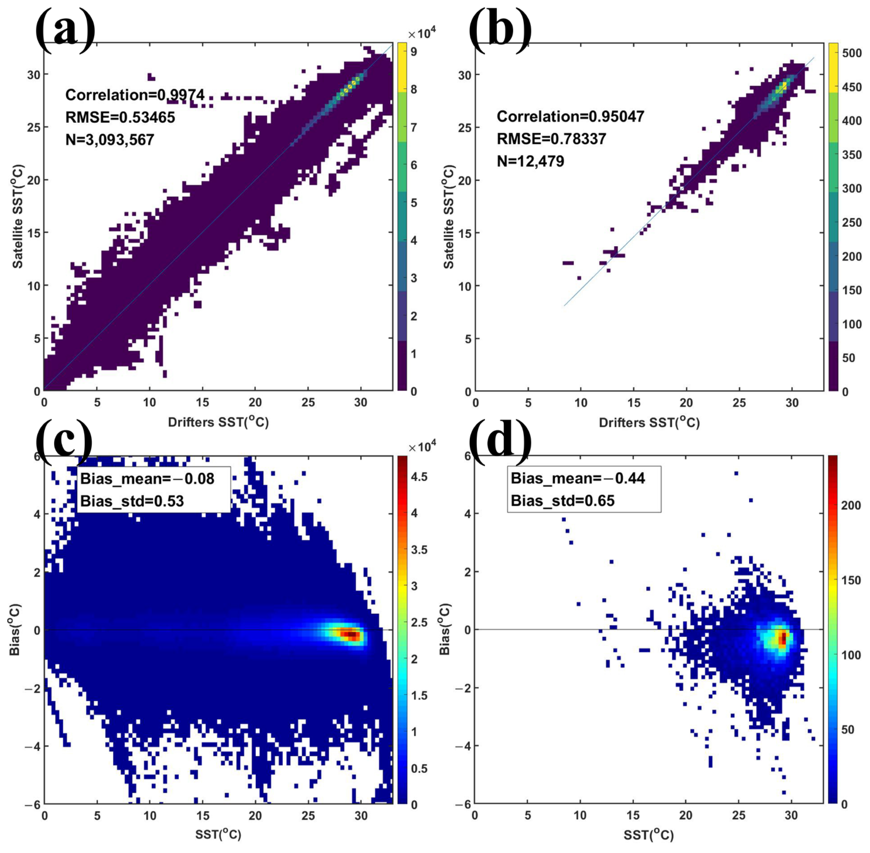
3.1. Validation of Satellite-Observed SSTs

Before the examination of the relationship between ESSTDs and the consequential TC intensity changes, the capability of capturing ESSTDs through the satellite-retrieved SST should be validated, particularly under the severe weather conditions accompanying TC passages. Figure 1a shows a comparison of satellite-observed microwave SSTs and all available in situ SSTs measured via the temperature meter onboard surface drifters [30] passing the study area during the entire study period. In total, 3,093,567 in situ SST measurements were collected and processed for validation, as shown in this analysis. The correlation coefficient obtained between the SSTs retrieved from satellite and in situ measurements is 0.997 (with a root-mean-square error (RMSE) of 0.535 °C), which indicates great consistency between the SSTs derived from satellite-based microwave sensors and surface drifters. Moreover, Figure 1b shows the same comparison for the periods of TC passages only (drifters in the 4° × 4° box area around the TC center, with 12,479 samples). The comparison shows generally the same consistency between the datasets. The correlation coefficient is 0.950 (with an RMSE of 0.783 °C). Figure 1c,d illustrate the bias between satellite-observed microwave SSTs and in situ SSTs. Under two different conditions, the mean bias is −0.08 and −0.44, suggesting a weak cold bias in satellite-observed sea surface temperatures relative to actual measurements, particularly noticeable during periods influenced by typhoons. The analysis shows the robustness of the usage of OISSTs in revealing TC-induced SST variations in the study area.

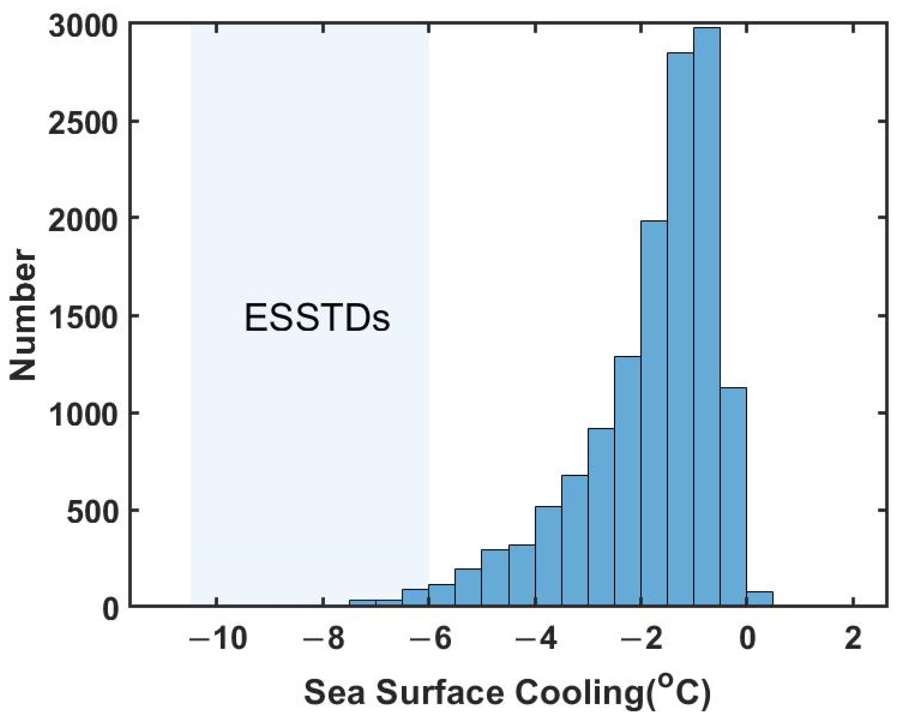
3.2. Characteristics of TICs and ESSTDs

Figure 2 shows the distribution of all the TICs corresponding to the TC passages in the WNP from 2001 to 2021. The figure shows that TICs occurred from 0 °C to stronger than −10 °C. TICs of −0.5–−1 °C occurred most frequently. The ratios of stronger cooling (for the TICs lower than −1 °C) gradually decrease. Moreover, as noted in the aforementioned section, only ~1% of the TICs (light-blue shaded area) are equal to or lower than −6 °C. Generally, the distribution of the TICs in the WNP shows great consistency with that proposed in a previous study but with a bias toward higher strength (see Figure 6 in the work of Dare and Mcbride [31]). The bias is attributed to the slight differences in sensors, the corresponding retrieved algorithms for satellite-based SSTs among different products, and the inherent inter-basin discrepancy of TICs in all basins in the world, as noted by Foltz et al. [32].

3.3. TICs and ESSTDs vs. Sharp TC Intensity Changes

The SST cooling induced by a TC passage can reduce the consequential TC intensity, which has been documented through either theory, observations, or numerical modeling [6,33,34,35]. However, as mentioned above, a comprehensive examination of the association between the TICs and the consequential TC intensity changes remains lacking, particularly for extreme TICs (ESSTDs). To further clarify the association between TICs, ESSTDs, and the consequential TC intensity development, Figure 3 shows a comparison between the TICs and the TC intensity changes (in delta wind speed). The TC intensity changes were identified by the wind speed variations within 24 h relative to the original wind speed corresponding to the TC center passing a certain position (where cooling takes place). Figure 3 shows that the wind speed modulations (TC intensity changes) display a near-linear dependence and good consistency with the TICs. Following a one-way analysis of variance (ANOVA) on the seven groups, a significant disparity in the mean TCI values among these groups was observed (F-statistic = 188.0614, p-value = 5.4645 × 10−229). Subsequent multiple comparison (post hoc) analysis revealed a statistically significant difference (p < 0.05) in the mean delta wind speed between ESSTDs and the 0 to −4 °C TICs. Generally, the stronger the TIC is, the stronger the reduction in wind forcing is. The relationship between the TIC and TC intensity changes has also been observed in previous studies [34,35]. This phenomenon implies that ESSTD plays a crucial role in sharp TC intensity changes.
The systematic analysis supports the negative impacts of SST drop on TC intensity changes (e.g., Lee and Chen [6]), particularly the SST drops belonging to ESSTDs (light-blue shaded area in Figure 2). Thus, a deeper understanding of the distributed characteristics and generated mechanism(s) of the ESSTDs plays a crucial role in improving the prediction of transient TC intensity changes. To obtain further information about the appearances of ESSTDs, the general characteristics of ESSTDs are revealed in the following section. Then, the appearances of abnormal ESSTDs are analyzed to elucidate the possible new mechanism(s) contributing to the generation of ESSTDs in addition to the existing theories.

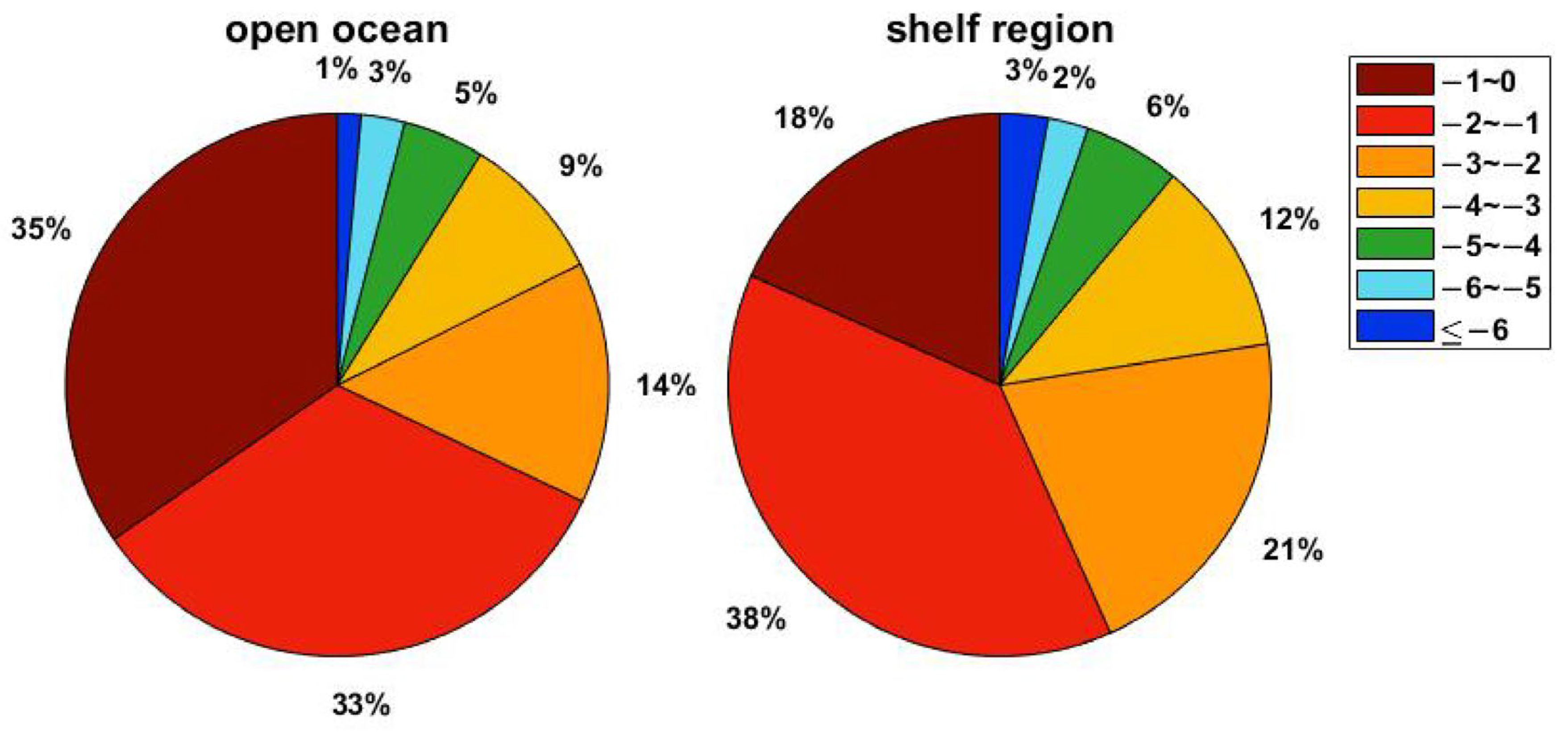
3.4. TICs and ESSTDs: Open Ocean versus Continental Shelf

Figure 4 shows the distributed ratios of all the TICs (including ESSTDs) corresponding to open ocean and shelf regions. In the open ocean (left plot in Figure 4), TICs less than 1 °C account for ~35% of the total number of TICs. For the shelf region (right plot in Figure 4), TICs between 1 °C and 2 °C account for 38% (the largest proportion) of the TICs. In general, the TICs that occurred in the open ocean with different strengths are weaker than those that took place in the shelf regions. The blue patches (ESSTDs) in both pie plots indicate that the frequency of ESSTDs in the shelf region is much higher than that in the open ocean. This phenomenon implies that the shelf region provides a relatively favorable environment for TC to trigger strong cooling. This pattern shows great consistency with the results of previous studies (e.g., Mitchell et al. [36]; Teague et al. [37]), which are largely based on comprehensive observed evidence.
Figure 5 shows the locations of the TICs that occurred in the shelf regions (green dots) and the open ocean (blue dots). Yellow and red dots denote the locations where ESSTDs occurred in the shelf regions and the open ocean, respectively. Some areas have no TICs because they do not belong to either shelf regions or open oceans by our definition. Overall, the number of blue dots is greater than that of green dots, implying that more TICs occurred in the open ocean than in the shelf regions from 2001 to 2021. Furthermore, more ESSTDs occurred in the shelf regions than in the open ocean. According to Mitchell et al. [36] and Figure 4, ESSTDs occurred more frequently in the shelf regions than in the open ocean because of the shallow bathymetry, the more complex wind–bathymetry, and the wind–regional current interactions. As previously mentioned, relative to the ESSTDs that occurred in the shelf regions, the ESSTDs that occurred in the open ocean are not physically straightforward. Thus, they largely attracted our attention. In the following section, one of the key targets is to explain why TCs lead to ESSTDs in the open ocean, where its background environment is unfavorable for conventional TCs triggering strong SST drops.
Table 1 shows the background information during the passages of the TC-triggered ESSTDs in the open ocean. Basically, these events lead to ESSTDs because of their individually favorable conditions, as documented in previous studies, such as a particularly slow translation speed, large TC size, strong TC intensities, double impacts of a previous storm, and potential influences of preexisting cyclonic eddies or subsurface thermal structures (e.g., Price [13]; Price et al. [38]; Babin et al. [39]; Walker et al. [40]; Lin et al. [41]; Zheng et al. [42,43]; Zheng et al. [7]; Kuo et al. [9]; Shen et al. [28]; Zhang et al. [44]). Based on preliminary examination, TC Kilo (2015) was identified as a non-typical ESSTD event with a regular translation speed and a relatively weak intensity, without any of the aforementioned favorable conditions.

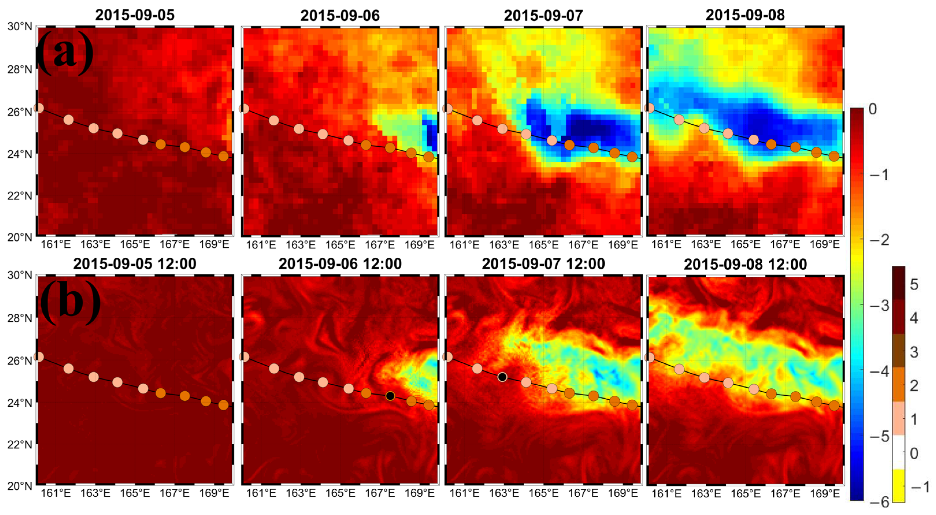
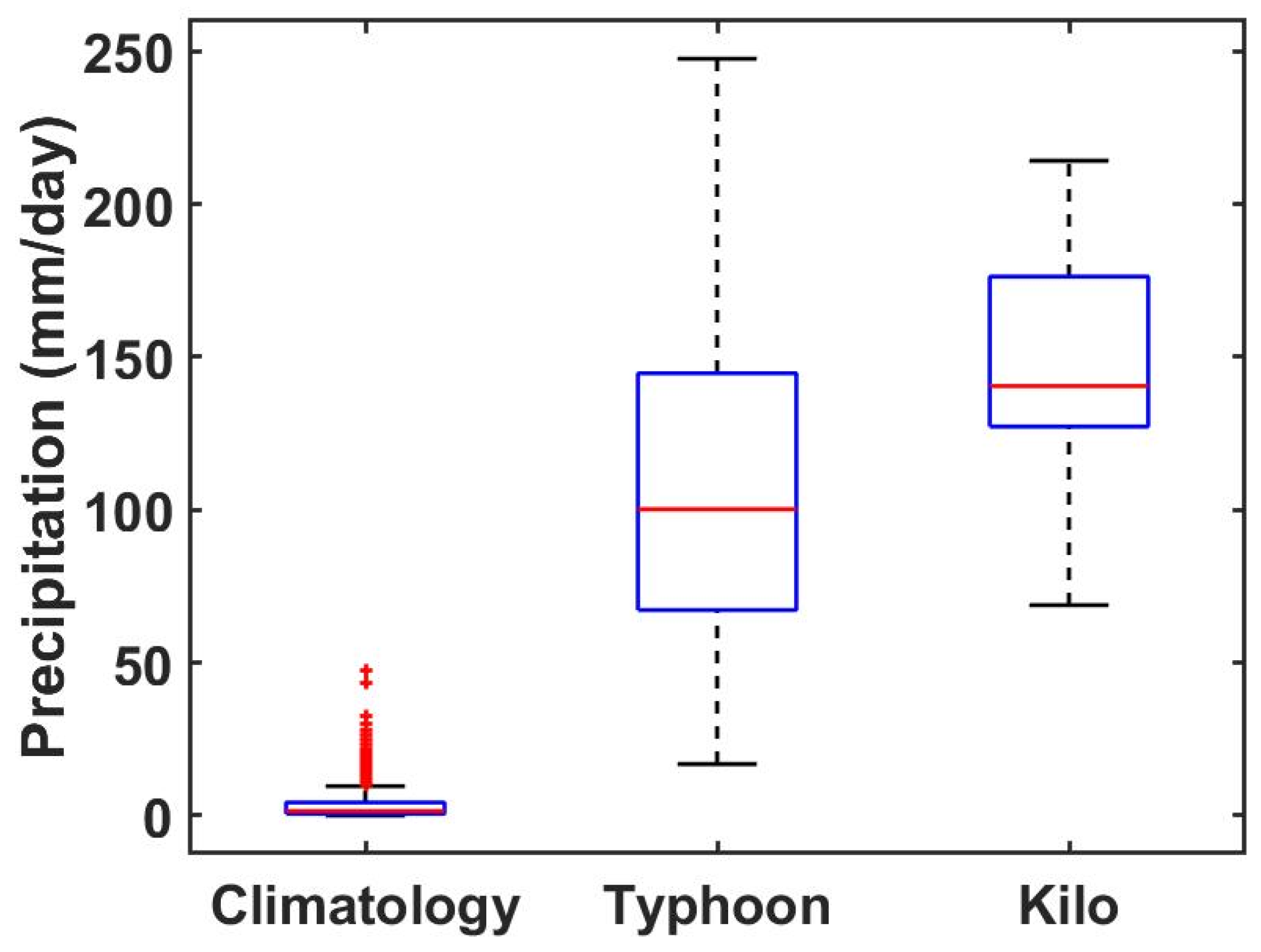
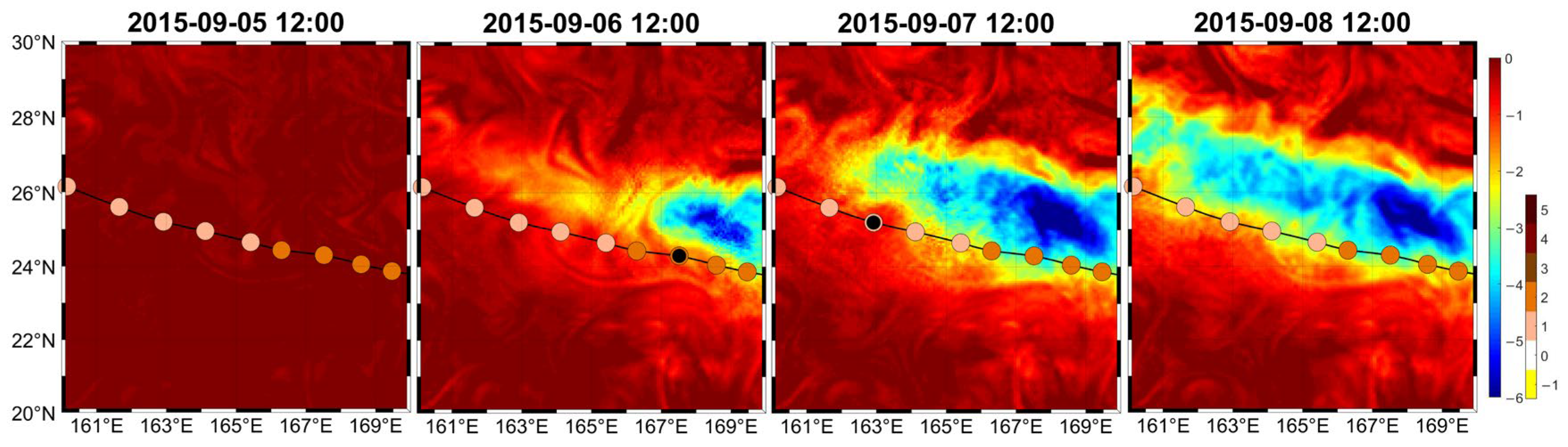
4. Outlier—Kilo (2015)

To further examine why Kilo triggered an ESSTD without distinct favorable conditions, a numerical experiment based on the ROMS was carried out to reconstruct the oceanic environment corresponding to the duration of the Kilo-induced ESSTD in the open ocean. Figure 6b shows the model simulation of the complete progression of the ESSTD to the passage of Kilo. For comparison, the cooling progression due to Kilo retrieved from satellite observations is also shown in Figure 6a. In general, the consistency of the pattern, timing, and evolution of the SST cooling after the Kilo passage indicates that the model simulation substantially reproduced the main progression of cooling in the case of Kilo.
Nevertheless, referring to the magnitudes of cooling progression, the ROMS seems to have not completely reconstructed the Kilo-induced cooling as shown in the satellite observations. On the basis of the model skill demonstrated in recent studies [27,28,29], the ROMS surprisingly failed to completely reproduce the magnitude of ESSTD due to Kilo. By examining the internal dynamics of the ROMS further, we found that the influence of rainfall might not be addressed adequately in the ROMS. Previous studies pointed out that precipitation influences the buoyancy of the ocean surface layer by transforming the salinity and temperature distribution. In addition, on the one hand, it would induce oceanic rainfall sensible heat flux (QP) leaving the ocean, while raindrop cools the sea surface [45,46,47]. On the other hand, the freshwater input of rain can enhance the stratification of the water column, consequently suppressing the vertical mixing of colder water from below, while the winds accompanied with TCs tend to induce vertical mixing in the upper ocean [46,48].
In the ROMS, a scheme related to rainfall is used to handle the effect of rainfall dilution and the decrease in salinity near the sea surface, which influence the density and consequential vertical stratification [49]. This effect is well documented in the papers of Jacob and Koblinsky [46] and Balaguru et al. [48]. In contrast, the dynamics of the ROMS do not include the effect of raindrop-driven surface cooling through the induction of sensible heat flux into the ocean, given the possible colder temperature of raindrops relative to the warmer sea surface temperature [45,47]. Heat-flux-driven sea surface cooling is generally considered to have a minor effect on SST modification [13,44,48]. However, it has been shown that the rainfall sensible heat flux can be as high as 200 W m−2 during intense rainfall events relative to the average heat flux of approximately 2.5 W m−2 from rainfall over the entire TOGA-COARE period [45], which indicates the potential of the heavy rainfall accompanied with TC passage to contribute marked SST drop through enhancing sensible heat flux. In a study by Ibrahim and Sun [47], they also indicated that Qp could be large at both short and long time scales, contrary to popular belief.
Notably, this effect has not been integrated into the ROMS dynamics [49]. Figure 7 shows the rainfall composites corresponding to the passage of Kilo (Kilo), all the TC passages through the domain of Kilo (Typhoon), and the climatological rainfall of the background environment (Climatology) in the area where Kilo passed through. The rainfall data used here were obtained from the Integrated Multi-satellite Retrievals for the GPM mission L3 daily accumulated precipitation (through http://apdrc.soest.hawaii.edu/, accessed on 23 September 2023) with a 0.25° × 0.25° spatial resolution. Among the three composites, Kilo is undoubtedly a heavy rainfall event. The medians of the three composites are 1.5, 100.2, and 140.5 mm/day for climatology, typhoon, and Kilo, respectively. Notably, the precipitation during the passage of KILO is nearly a hundred times stronger than that corresponding to the climatological rainfall of the background environment. Thus, in this case, heat-flux-driven sea surface cooling should not be considered a minor effect on influencing the SST.
According to the theories of Gosnell et al. [45] and Jacob and Koblinsky [46], the aforementioned effect was estimated based on the oceanic precipitation sensible heat flux (Qp), the satellite observed rainfall data (R), and the mixed layer depth (MLD) data. Qp is expressed as follows:
Q p = c w ρ R × T r T s ,
where R (m s−1) is the rain rate, cw (4186 J kg−1 K−1) is the specific heat of the seawater, ρ (1000 kg m−3) denotes freshwater density, Tr (K) corresponds to the temperature of the rain drops, and Ts (K) is the SST. The rainfall caused by Kilo was synthesized from the maximum daily accumulated precipitation at each point during the entire TC period. In the analysis, we used ROMS SST before the TC approached (5 September) as Ts and 24.04 °C as Tr [46]. Here, the temperature of 24.04 °C was derived from the wet-bulb temperature of the 10 m air at 26°C and 85% humidity. According to Gosnell et al. [45], employing wet-bulb temperature as an estimation for rain temperature exhibits an error of approximately 0.1 W m−2 in the tropical Pacific region. Detailed precipitation along Kilo’s track and Qp can be seen Figure S1 in the Supplementary Material.
Afterward, to assess the effect of Qp-induced cooling during the duration of Kilo, according to Ibrahim and Sun [47], the average Qp was converted to temperature change in the mixed layer in the following relationship (Equation (2)).
T = ( t   Q p ) / ( c w ρ s w H ) ,
where ΔT is the temperature change resulting from the gathered Qp cooling in the MLD, Δt is the period of Kilo passage, ρsw is the seawater density, and H is the MLD (m). The MLD and ρsw data were derived from the product of the Argo mixed layer climatology obtained through http://mixedlayer.ucsd.edu/, accessed on 5 October 2023. Given that the TC rainfall preceded the extreme wind stress during Kilo, we assumed that the raindrop was not mixed well upon entering the subsurface before causing Qp cooling. Thus, the temperature correction provided by the estimation of ΔT remained near the sea surface (with the assumption of H of ~1 m). It is important to note that ΔT is heavily influenced by the thickness of the ocean mixed layer and the intensity of mixing. The impact of identical rainfall events may result in varying ΔT under different conditions (see ΔT under various mixing scenarios in Figure S2 in the Supplementary Material).
Figure 8 shows the model simulation that integrates the corrected terms contributed by Qp cooling. After integrating the effect, the cooling shows high-level consistency with the satellite-observed OISSTs (Figure 6a). The SST correction varies from 0.1 °C to 3.14 °C (with a mean of 0.36 °C) and largely improves the model simulation of the sea surface cooling due to Kilo. Generally, the result endorses the possibility of heavy rainfall events with the Kilo passage, contributing an additional SST drop to the momentum-driven mixing (Figure 6b) by enhancing the oceanic rainfall sensible heat flux (QP).

5. Conclusions and Remarks

The main results of the study are summarized as follows: (1) According to a comparison of the satellite observations and the in situ measurements, the usage of OISSTs shows robustness in revealing TC-induced SST variations. (2) The TICs in the WNP show great consistency with that proposed by Dare and Mcbride [31] but with a bias toward higher strength. This bias is attributed to the slightly different sensors, the corresponding retrieved algorithms for satellite-based SSTs among different products, and the inherent inter-basin discrepancy of the TICs in all the basins in the world, as reported by Foltz et al. [32]. (3) Wind speed modulations (TC intensity changes) show a near-linear dependence on the strength of the TICs. Generally, the stronger the TIC is, the stronger the reduction in wind forcing is. This systematic analysis supports the negative impacts of SST drops on TC intensity changes, particularly for the SST drops belonging to ESSTDs. (4) In the northwest Pacific region, TICs that occur in the open ocean are generally weaker than those that took place in the shelf regions, implying that the shelf region provides a favorable environment for TC triggering strong cooling. This notion shows great consistency with the results of previous studies but is based on comprehensive evidence.
Subsequently, the unexpected ESSTDs that occurred in the open ocean were systematically examined. Among them, Kilo (2015) was the only event that triggered an ESSTD during its lifespan without any documented favorable conditions. Numerical experiments based on the ROMS were then carried out to explore the possible mechanisms resulting in the ESSTD due to Kilo. The result indicates that the heavy rainfall that accompanied the passage of Kilo contributed an additional SST drop through the enhancement in oceanic rainfall sensible heat flux (QP) in addition to the momentum-driven cooling source from the subsurface.
According to previous studies, QP could be significant at both long and short time scales, and this process enhances the sensible heat flux into the upper ocean because the temperature of the raindrops could be much colder than the SST in the tropical ocean [45,46,47]. Zhang et al. [44] also indicated that some influence from surface fluxes may exist, particularly for the duration of weak storms. Typhoon Kilo is an example of such an event with weak intensity but heavy rainfall during its passage. Moreover, Ibrahim and Sun [47] emphasized that apart from the cooling effect, the decrease in SST induced by Qp inhibits both the latent heat flux and sensible heat flux, consequently influencing the heat exchange cycle between the ocean and the atmosphere. In addition to the effect of the freshwater input of rain stratifying the water column and exhibiting vertical mixing [46,48], the effect of short-term heavy rainfall with storm passage leading to extra sea surface cooling deserves increased attention.

Supplementary Materials

The following supporting information can be downloaded at: https://www.mdpi.com/article/10.3390/rs16010205/s1, Figure S1: Detailed precipitation and Qp; Figure S2: ΔT under various mixing scenarios.

Author Contributions

Conceptualization, Z.-W.Z., Y.-C.T. and D.-G.L.; Methodology, J.-Y.L., Z.-W.Z., Y.-C.T. and D.-G.L.; Software, J.-Y.L. and H.H.; Validation, J.-Y.L.; Formal analysis, J.-Y.L. and H.H.; Writing—original draft, J.-Y.L. and Z.-W.Z.; Visualization, J.-Y.L. and H.H.; Supervision, Z.-W.Z. All authors have read and agreed to the published version of the manuscript.

Funding

This research was funded by Taiwan’s Ministry of Science and Technology (MOST) under 111-2611-M-003-003-MY3.

Data Availability Statement

The data presented in this study are available on request from the corresponding author.

Conflicts of Interest

The authors declare no conflicts of interest.

References

  1. Chien, F.-C.; Kuo, H.-C. On the Extreme Rainfall of Typhoon Morakot (2009). J. Geophys. Res. Atmos. 2011, 116. [Google Scholar] [CrossRef]
  2. Schade, L.R.; Emanuel, K.A. The Ocean’s Effect on the Intensity of Tropical Cyclones: Results from a Simple Coupled Atmosphere–Ocean Model. J. Atmos. Sci. 1999, 56, 642–651. [Google Scholar] [CrossRef]
  3. Shay, L.K.; Goni, G.J.; Black, P.G. Effects of a Warm Oceanic Feature on Hurricane Opal. Mon. Weather. Rev. 2000, 128, 1366–1383. [Google Scholar] [CrossRef]
  4. Wu, C.-C.; Lee, C.-Y.; Lin, I.-I. The Effect of the Ocean Eddy on Tropical Cyclone Intensity. J. Atmos. Sci. 2007, 64, 3562–3578. [Google Scholar] [CrossRef]
  5. Lin, I.-I.; Wu, C.-C.; Pun, I.-F.; Ko, D.-S. Upper-Ocean Thermal Structure and the Western North Pacific Category 5 Typhoons. Part I: Ocean Features and the Category 5 Typhoons’ Intensification. Mon. Weather Rev. 2008, 136, 3288–3306. [Google Scholar] [CrossRef]
  6. Lee, C.-Y.; Chen, S.S. Stable Boundary Layer and Its Impact on Tropical Cyclone Structure in a Coupled Atmosphere–Ocean Model. Mon. Weather Rev. 2014, 142, 1927–1944. [Google Scholar] [CrossRef]
  7. Zheng, Z.-W.; Lin, I.-I.; Wang, B.; Huang, H.-C.; Chen, C.-H. A Long Neglected Damper in the El Niño—Typhoon Relationship: A ‘Gaia-Like’ Process. Sci. Rep. 2015, 5, 11103. [Google Scholar] [CrossRef] [PubMed]
  8. Glenn, S.M.; Miles, T.N.; Seroka, G.N.; Xu, Y.; Forney, R.K.; Yu, F.; Roarty, H.; Schofield, O.; Kohut, J. Stratified Coastal Ocean Interactions with Tropical Cyclones. Nat. Commun. 2016, 7, 10887. [Google Scholar] [CrossRef]
  9. Kuo, Y.-C.; Zheng, Z.-W.; Zheng, Q.; Gopalakrishnan, G.; Lee, H.-Y. Typhoon–Kuroshio Interaction in an Air–Sea Coupled System: Case Study of Typhoon Nanmadol (2011). Ocean. Model. 2018, 132, 130–138. [Google Scholar] [CrossRef]
  10. Emanuel, K.A. Thermodynamic Control of Hurricane Intensity. Nature 1999, 401, 665–669. [Google Scholar] [CrossRef]
  11. Zhu, T.; Zhang, D.-L. The Impact of the Storm-Induced SST Cooling on Hurricane Intensity. Adv. Atmos. Sci. 2006, 23, 14–22. [Google Scholar] [CrossRef]
  12. Mohanty, S.; Nadimpalli, R.; Osuri, K.K.; Pattanayak, S.; Mohanty, U.C.; Sil, S. Role of Sea Surface Temperature in Modulating Life Cycle of Tropical Cyclones over Bay of Bengal. Trop. Cyclone Res. Rev. 2019, 8, 68–83. [Google Scholar] [CrossRef]
  13. Price, J.F. Upper Ocean Response to a Hurricane. J. Phys. Oceanogr. 1981, 11, 153–175. [Google Scholar] [CrossRef]
  14. Zedler, S.E.; Dickey, T.D.; Doney, S.C.; Price, J.F.; Yu, X.; Mellor, G.L. Analyses and Simulations of the Upper Ocean’s Response to Hurricane Felix at the Bermuda Testbed Mooring Site: 13–23 August 1995. J. Geophys. Res. Oceans 2002, 107, 25-1–25-29. [Google Scholar] [CrossRef]
  15. Lin, I.-I.; Liu, W.T.; Wu, C.-C.; Wong, G.T.F.; Hu, C.; Chen, Z.; Liang, W.-D.; Yang, Y.; Liu, K.-K. New Evidence for Enhanced Ocean Primary Production Triggered by Tropical Cyclone. Geophys. Res. Lett. 2003, 30. [Google Scholar] [CrossRef]
  16. Black, P.G.; D’Asaro, E.A.; Drennan, W.M.; French, J.R.; Niiler, P.P.; Sanford, T.B.; Terrill, E.J.; Walsh, E.J.; Zhang, J.A. Air–Sea Exchange in Hurricanes: Synthesis of Observations from the Coupled Boundary Layer Air–Sea Transfer Experiment. Bull. Amer. Meteor. Soc. 2007, 88, 357–374. [Google Scholar] [CrossRef]
  17. D’Asaro, E.A.; Sanford, T.B.; Niiler, P.P.; Terrill, E.J. Cold Wake of Hurricane Frances. Geophys. Res. Lett. 2007, 34. [Google Scholar] [CrossRef]
  18. Zheng, Z.-W.; Lin, J.-Y.; Gopalakrishnan, G.; Chen, Y.-R.; Doong, D.-J.; Ho, C.-R.; Zheng, Q.; Wu, C.-R.; Huang, C.-F. Extreme Cooling of 12.5 °C Triggered by Typhoon Fungwong (2008). Ocean Model. 2023, 182, 102176. [Google Scholar] [CrossRef]
  19. Lumpkin, R.; Centurioni, L. NOAA Global Drifter Program Quality-Controlled 6-Hour Interpolated Data from Ocean Surface Drifting Buoys; NOAA National Centers for Environmental Information: Asheville, NC, USA, 2019.
  20. Perez, R.C.; Foltz, G.R.; Lumpkin, R.; Wei, J.; Voss, K.J.; Ondrusek, M.; Wang, M.; Bourassa, M.A. Chapter 5—Oceanographic Buoys: Providing Ocean Data to Assess the Accuracy of Variables Derived from Satellite Measurements. In Field Measurements for Passive Environmental Remote Sensing; Nalli, N.R., Ed.; Elsevier: Amsterdam, The Netherlands, 2023; pp. 79–100. [Google Scholar]
  21. Hansen, D.V.; Poulain, P.-M. Quality Control and Interpolations of WOCE-TOGA Drifter Data. J. Atmos. Ocean. Technol. 1996, 13, 900–909. [Google Scholar] [CrossRef]
  22. Large, W.G.; McWilliams, J.C.; Doney, S.C. Oceanic Vertical Mixing: A Review and a Model with a Nonlocal Boundary Layer Parameterization. Rev. Geophys. 1994, 32, 363–403. [Google Scholar] [CrossRef]
  23. Gelaro, R.; McCarty, W.; Suárez, M.J.; Todling, R.; Molod, A.; Takacs, L.; Randles, C.A.; Darmenov, A.; Bosilovich, M.G.; Reichle, R.; et al. The Modern-Era Retrospective Analysis for Research and Applications, Version 2 (MERRA-2). J. Clim. 2017, 30, 5419–5454. [Google Scholar] [CrossRef] [PubMed]
  24. Cummings, J.A. Operational Multivariate Ocean Data Assimilation. Q. J. R. Meteorol. Soc. 2005, 131, 3583–3604. [Google Scholar] [CrossRef]
  25. Shchepetkin, A.F.; McWilliams, J.C. A Method for Computing Horizontal Pressure-Gradient Force in an Oceanic Model with a Nonaligned Vertical Coordinate. J. Geophys. Res. Oceans 2003, 108. [Google Scholar] [CrossRef]
  26. Shchepetkin, A.F.; McWilliams, J.C. The Regional Oceanic Modeling System (ROMS): A Split-Explicit, Free-Surface, Topography-Following-Coordinate Oceanic Model. Ocean Model. 2005, 9, 347–404. [Google Scholar] [CrossRef]
  27. Zheng, Z.-W.; Zheng, Q.; Lee, C.-Y.; Gopalakrishnan, G. Transient Modulation of Kuroshio Upper Layer Flow by Directly Impinging Typhoon Morakot in East of Taiwan in 2009. J. Geophys. Res. Oceans 2014, 119, 4462–4473. [Google Scholar] [CrossRef]
  28. Shen, D.; Li, X.; Wang, J.; Bao, S.; Pietrafesa, L.J. Dynamical Ocean Responses to Typhoon Malakas (2016) in the Vicinity of Taiwan. J. Geophys. Res. Oceans 2021, 126, e2020JC016663. [Google Scholar] [CrossRef]
  29. Zheng, Z.-W.; Chen, Y.-R. Influences of Tidal Effect on Upper Ocean Responses to Typhoon Passages Surrounding Shore Region off Northeast Taiwan. J. Mar. Sci. Eng. 2022, 10, 1419. [Google Scholar] [CrossRef]
  30. Elipot, S.; Lumpkin, R.; Perez, R.C.; Lilly, J.M.; Early, J.J.; Sykulski, A.M. A Global Surface Drifter Data Set at Hourly Resolution. J. Geophys. Res. Oceans 2016, 121, 2937–2966. [Google Scholar] [CrossRef]
  31. Dare, R.A.; McBride, J.L. Sea Surface Temperature Response to Tropical Cyclones. Mon. Weather. Rev. 2011, 139, 3798–3808. [Google Scholar] [CrossRef]
  32. Foltz, G.R.; Balaguru, K.; Hagos, S. Interbasin Differences in the Relationship between SST and Tropical Cyclone Intensification. Mon. Weather Rev. 2018, 146, 853–870. [Google Scholar] [CrossRef]
  33. Bender, M.A.; Ginis, I. Real-Case Simulations of Hurricane–Ocean Interaction Using A High-Resolution Coupled Model: Effects on Hurricane Intensity. Mon. Weather Rev. 2000, 128, 917–946. [Google Scholar] [CrossRef]
  34. Cione, J.J.; Uhlhorn, E.W. Sea Surface Temperature Variability in Hurricanes: Implications with Respect to Intensity Change. Mon. Weather Rev. 2003, 131, 1783–1796. [Google Scholar] [CrossRef]
  35. Lloyd, I.D.; Vecchi, G.A. Observational Evidence for Oceanic Controls on Hurricane Intensity. J. Clim. 2011, 24, 1138–1153. [Google Scholar] [CrossRef]
  36. Mitchell, D.A.; Teague, W.J.; Jarosz, E.; Wang, D.W. Observed Currents over the Outer Continental Shelf during Hurricane Ivan. Geophys. Res. Lett. 2005, 32. [Google Scholar] [CrossRef]
  37. Teague, W.J.; Jarosz, E.; Wang, D.W.; Mitchell, D.A. Observed Oceanic Response over the Upper Continental Slope and Outer Shelf during Hurricane Ivan. J. Phys. Oceanogr. 2007, 37, 2181–2206. [Google Scholar] [CrossRef]
  38. Price, J.F. Internal Wave Wake of a Moving Storm. Part I. Scales, Energy Budget and Observations. J. Phys. Oceanogr. 1983, 13, 949–965. [Google Scholar] [CrossRef]
  39. Babin, S.M.; Carton, J.A.; Dickey, T.D.; Wiggert, J.D. Satellite Evidence of Hurricane-Induced Phytoplankton Blooms in an Oceanic Desert. J. Geophys. Res. Oceans 2004, 109. [Google Scholar] [CrossRef]
  40. Walker, N.D.; Leben, R.R.; Balasubramanian, S. Hurricane-Forced Upwelling and Chlorophyll a Enhancement within Cold-Core Cyclones in the Gulf of Mexico. Geophys. Res. Lett. 2005, 32. [Google Scholar] [CrossRef]
  41. Lin, I.-I.; Wu, C.-C.; Emanuel, K.A.; Lee, I.-H.; Wu, C.-R.; Pun, I.-F. The Interaction of Supertyphoon Maemi (2003) with a Warm Ocean Eddy. Mon. Weather Rev. 2005, 133, 2635–2649. [Google Scholar] [CrossRef]
  42. Zheng, Z.-W.; Ho, C.-R.; Zheng, Q.; Lo, Y.-T.; Kuo, N.-J.; Gopalakrishnan, G. Effects of Preexisting Cyclonic Eddies on Upper Ocean Responses to Category 5 Typhoons in the Western North Pacific. J. Geophys. Res. Oceans 2010, 115. [Google Scholar] [CrossRef]
  43. Zheng, Z.-W.; Ho, C.-R.; Zheng, Q.; Kuo, N.-J.; Lo, Y.-T. Satellite Observation and Model Simulation of Upper Ocean Biophysical Response to Super Typhoon Nakri. Cont. Shelf Res. 2010, 30, 1450–1457. [Google Scholar] [CrossRef]
  44. Zhang, H.; He, H.; Zhang, W.-Z.; Tian, D. Upper Ocean Response to Tropical Cyclones: A Review. Geosci. Lett. 2021, 8, 1. [Google Scholar] [CrossRef]
  45. Gosnell, R.; Fairall, C.W.; Webster, P.J. The Sensible Heat of Rainfall in the Tropical Ocean. J. Geophys. Res. Oceans 1995, 100, 18437–18442. [Google Scholar] [CrossRef]
  46. Jacob, S.D.; Koblinsky, C.J. Effects of Precipitation on the Upper-Ocean Response to a Hurricane. Mon. Weather Rev. 2007, 135, 2207–2225. [Google Scholar] [CrossRef]
  47. Ibrahim, H.D.; Sun, Y. Sea Surface Cooling by Rainfall Modulates Earth’s Heat Energy Flow. J. Clim. 2023, 36, 5125–5141. [Google Scholar] [CrossRef]
  48. Balaguru, K.; Foltz, G.R.; Leung, L.R.; Hagos, S.M. Impact of Rainfall on Tropical Cyclone-Induced Sea Surface Cooling. Geophys. Res. Lett. 2022, 49, e2022GL098187. [Google Scholar] [CrossRef]
  49. Hedström, K.S. Technical Manual for a Coupled Sea-Ice/Ocean Circulation Model (Version 3); Contract No. M07PC13368; US Department of the Interior Minerals Management Service Anchorage: Anchorage, AK, USA, 2009.
Figure 1. (a) Comparison of satellite-based OISST and available in situ SSTs measured via all surface drifters passing the study area from 2001 to 2021 (3,093,567 samples). (b) Comparison for the periods of TC passages regardless of the season (12,479 samples). (c,d) As in (a,b) but representing the bias between the satellite-based OISST and drifters (satellite–drifter). The color bar indicates the number of each bin.
Remotesensing 16 00205 g001
Figure 2. Number distribution of TICs with individual strengths corresponding to all TC passages in the WNP from 2001 to 2021. The box area outlines the TICs that belong to ESSTDs.
Remotesensing 16 00205 g002
Figure 3. Comparison of TICs (unit: °C) and TCI changes in delta wind speed (unit: ms−1). The blue dots show the means of each interval. The red bars show the 95% confidence interval, and the 25th and 75th percentiles are marked by black asterisks.
Remotesensing 16 00205 g003
Figure 4. Ratios of all TICs (including ESSTDs) corresponding to open ocean (left) and shelf regions (right).
Remotesensing 16 00205 g004
Figure 5. Distribution of all TICs in the shelf region (green dots) and open ocean (blue dots). Yellow and red dots denote ESSTDs that occurred in the shelf region and open ocean, respectively. ESSTDs that occurred in the open ocean (red dots) were triggered by the typhoons listed in Table 1.
Remotesensing 16 00205 g005
Figure 6. Sea surface cooling responses (relative to 4 September) during the passage of Kilo (2015) via (a) satellite-based OISSTs and (b) ROMS simulation. Color shades denote SSTs (left color bar) (unit: °C). TC intensities are marked with color dots (right color bar). Black dots denote the central positions of Kilo.
Remotesensing 16 00205 g006
Figure 7. Daily accumulated precipitation in different composites. Climatology is the domain (20–30°N, 160–170°E) average in September climatology. Typhoon is the average precipitation composite calculated from all TCs passing through the same domain from 2001 to 2020. Kilo is the average precipitation along the track of Kilo in the domain. The red line in the blue box denotes the median, and the lower and upper boundaries denote the 25th percentile and 75th percentile, respectively. Whiskers above and below the box indicate the 75th percentile + 1.5 × IQR and 25th percentile − 1.5 × IQR, respectively, where IQR denotes the 75th percentile–25th percentile. The red plus signs denote the outliers.
Remotesensing 16 00205 g007
Figure 8. Model-simulated sea surface cooling responses (relative to 4 September 2015) during the passage of Kilo (2015) with corrected term due to Qp cooling. Color shades denote SSTs (left color bar) (unit: °C). TC intensities are marked with color dots (right color bar). Black dot denotes the central positions of Kilo.
Remotesensing 16 00205 g008
Table 1. Background information during the passages of all TC-triggered ESSTDs in the open ocean from 2001 to 2021.
NameDate△SST Intensity CategoryMoving Speed (m/s)Cyclonic Eddies (SSH < 0.2 m)Twice Impact *Previous TC **
MAN-YI6 August 2001−6.9222.57XXO
FENGSHEN23 July 2002 09:00−6.0537.72XXX
ELE4 September 2002−7.4221.54XXX
KETSANA21 October 2003−7.0521.54OXX
SOULIK13 October 2006−6.3811.03XXX
CHOI-WAN18 September 2009−6.5234.12XXX
MA-ON16 July 2011−7.2745.14XXX
PRAPIROON12 October 2012−6.9531.54OXX
SOULIK11 July 2013−6.8436.17OXX
NEOGURI7 July 2014−7.0256.69XXX
VONGFONG9 October 2014−6.1252.57OXX
ATSANI21 August 2015−6.4835.14XXX
KILO7 September 2015−6.3315.14XXX
DUJUAN25 September 2015−6.3611.54OXX
NORU31 July 2017−6.1742.57XXX
KROSA11 August 2019−7.102.57XXX
MINDULLE28 September 2021−6.423.09OXX
* Twice Impact is defined as TC track forming a loop and TC striking the same area twice. ** Previous TC is defined as whether a previous TC passed through the ESSTD area in the previous two weeks. The symbol “O” denotes compliance with favorable conditions, whereas “X” indicates non-compliance with favorable conditions.
Disclaimer/Publisher’s Note: The statements, opinions and data contained in all publications are solely those of the individual author(s) and contributor(s) and not of MDPI and/or the editor(s). MDPI and/or the editor(s) disclaim responsibility for any injury to people or property resulting from any ideas, methods, instructions or products referred to in the content.

