


Low-Tech and Low-Cost System for High-Resolution Underwater RTK Photogrammetry in Coastal Shallow Waters

 , , , , ,
Abstract
:1. Introduction
2. Study Areas
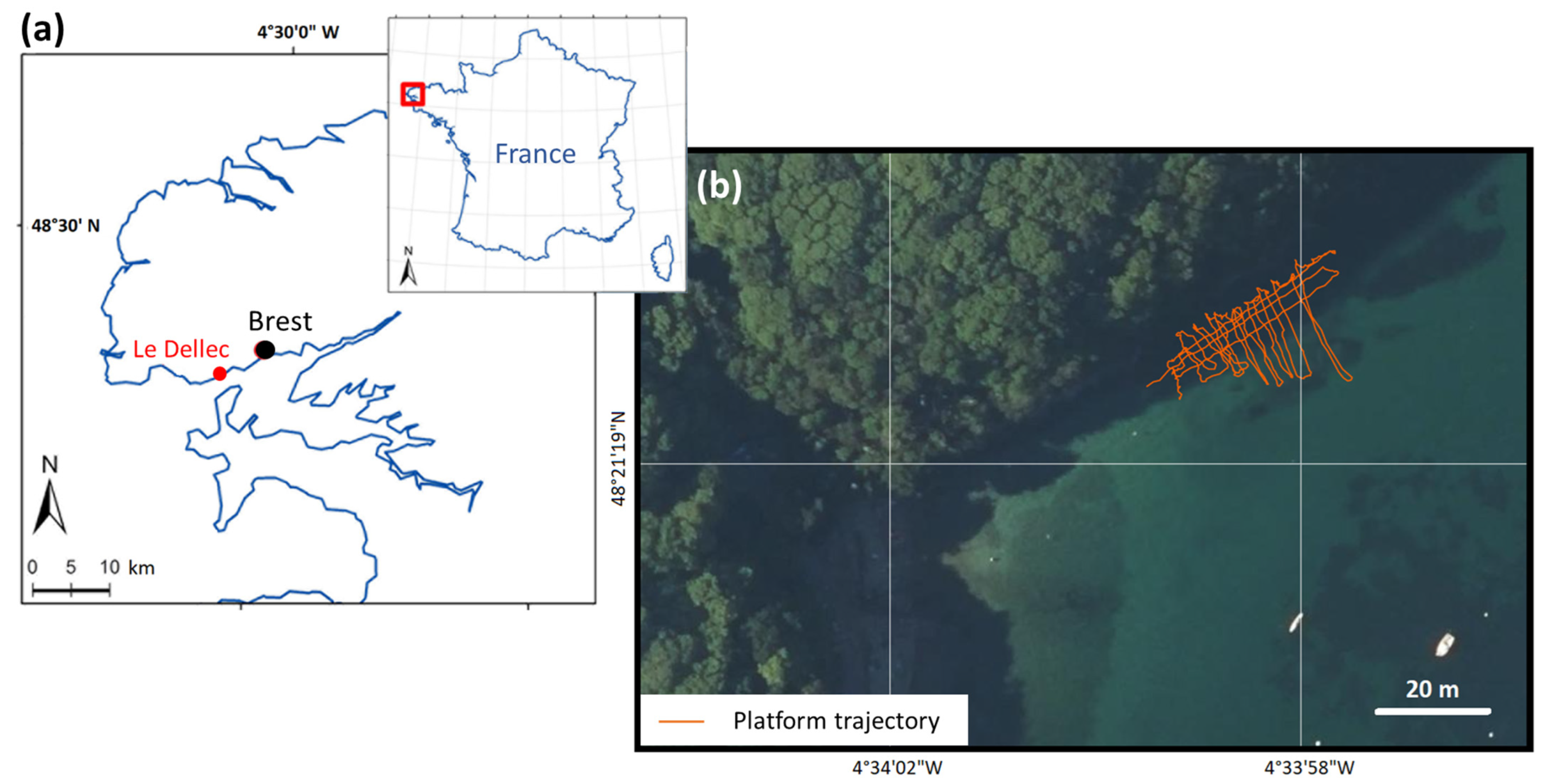
2.1. Method Validation Site: Dellec Bay
2.2. Test Site: Hermitage Backreef Zone
3. Material and Methods
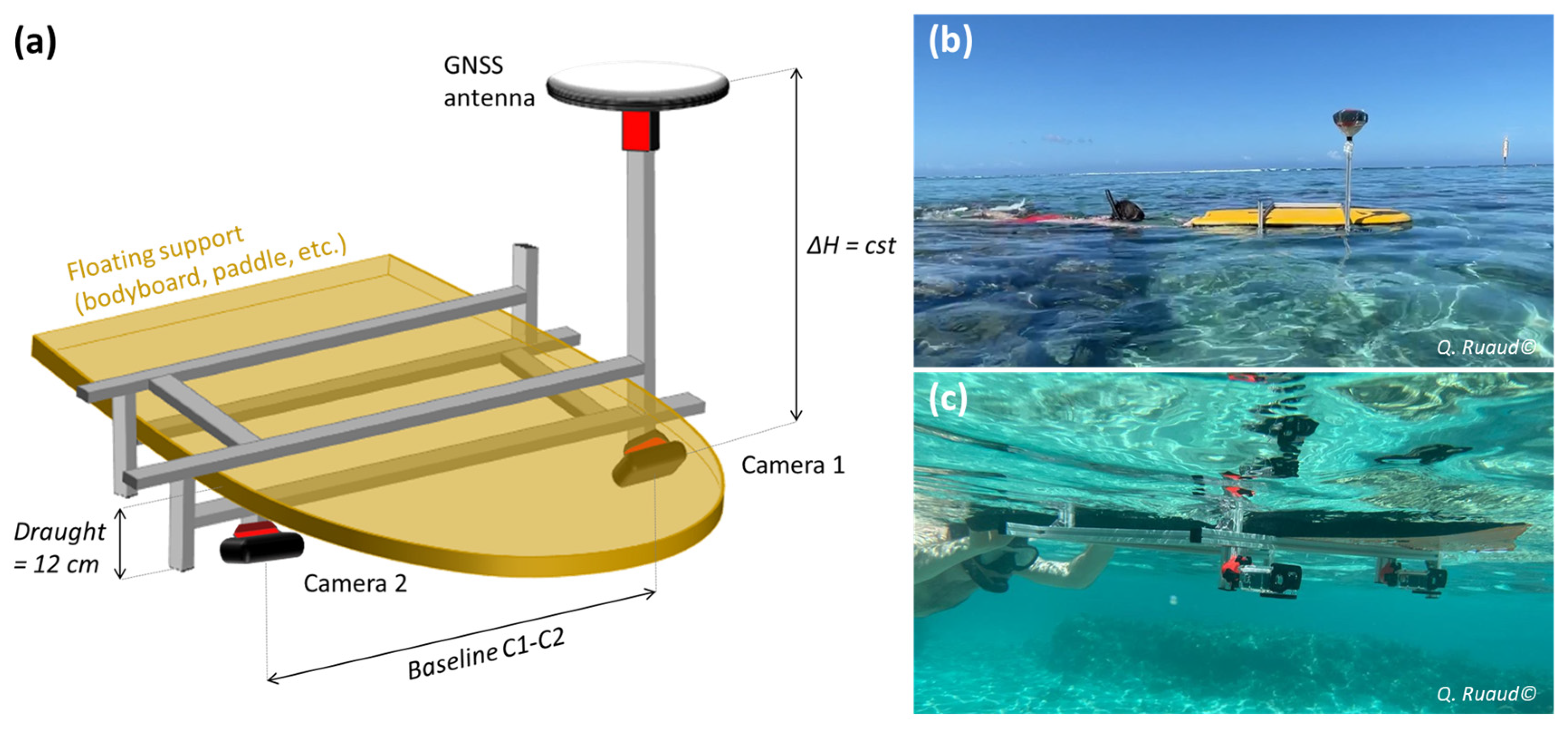
3.1. Principle of the Method
3.2. POSEIDON Platform
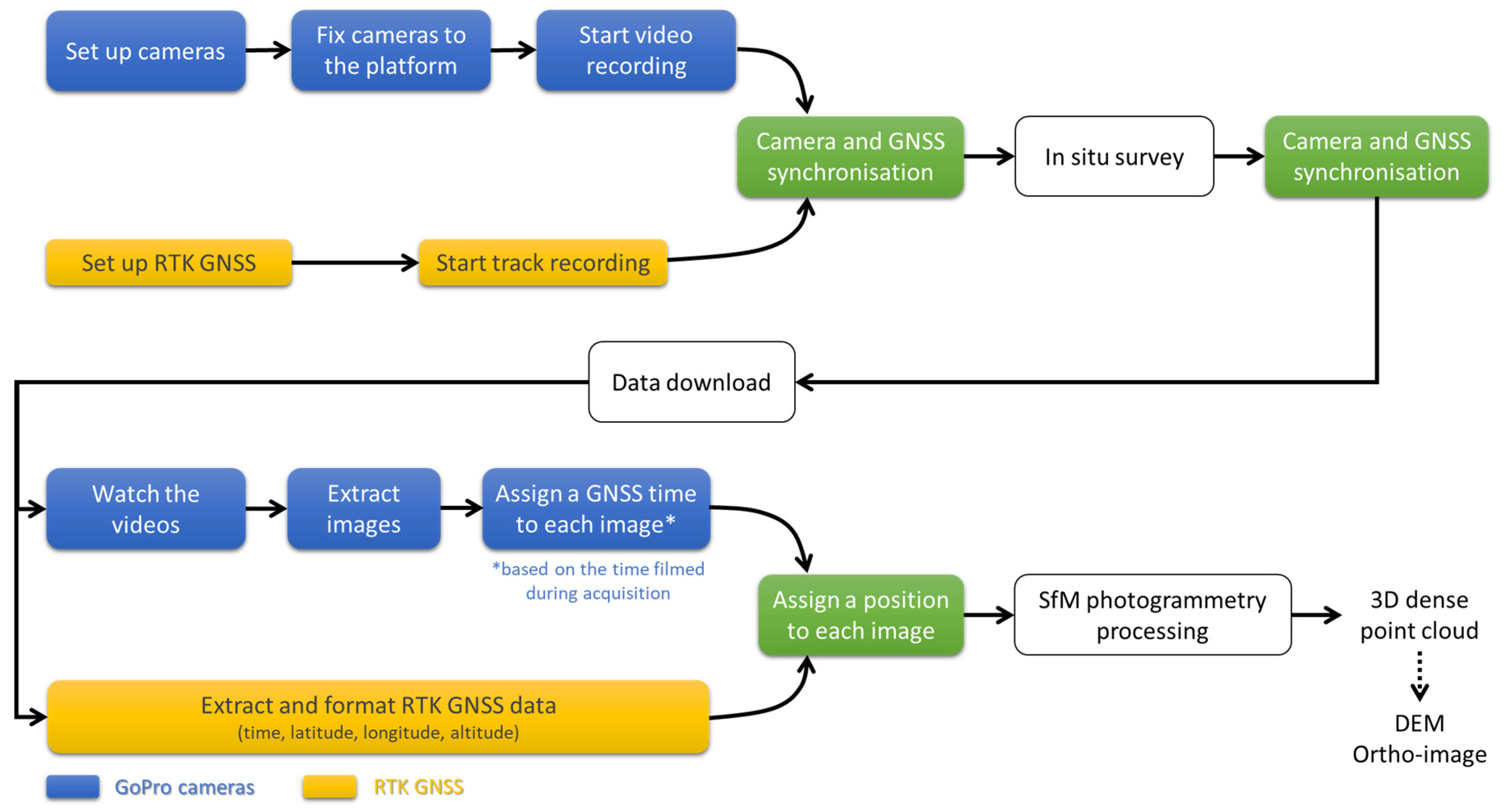
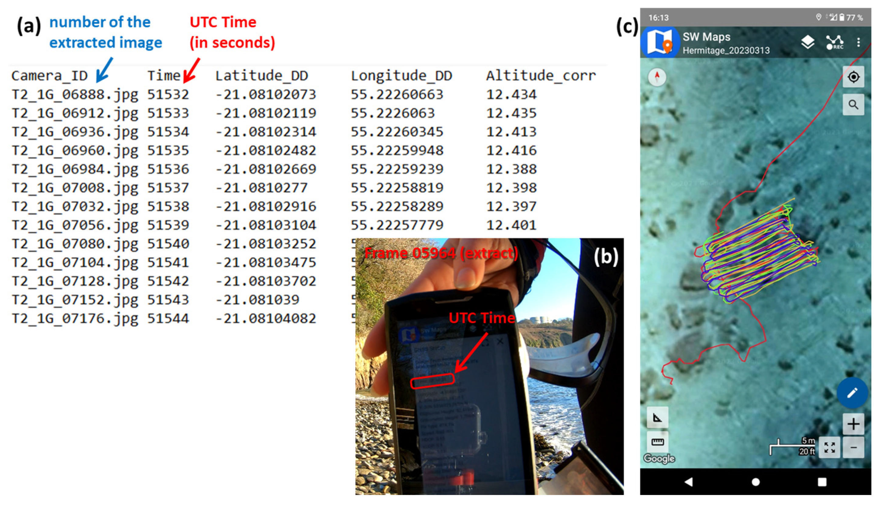
3.3. Practical Aspects of Acquisition and Processing
- In Dellec Bay: gradual variations in bathymetry were expected, with a water height of around 3 to 6 m. The two cameras were therefore pointed at the nadir and spaced as far apart as possible (58 cm). The speed of the platform was around 1.14 km/h.
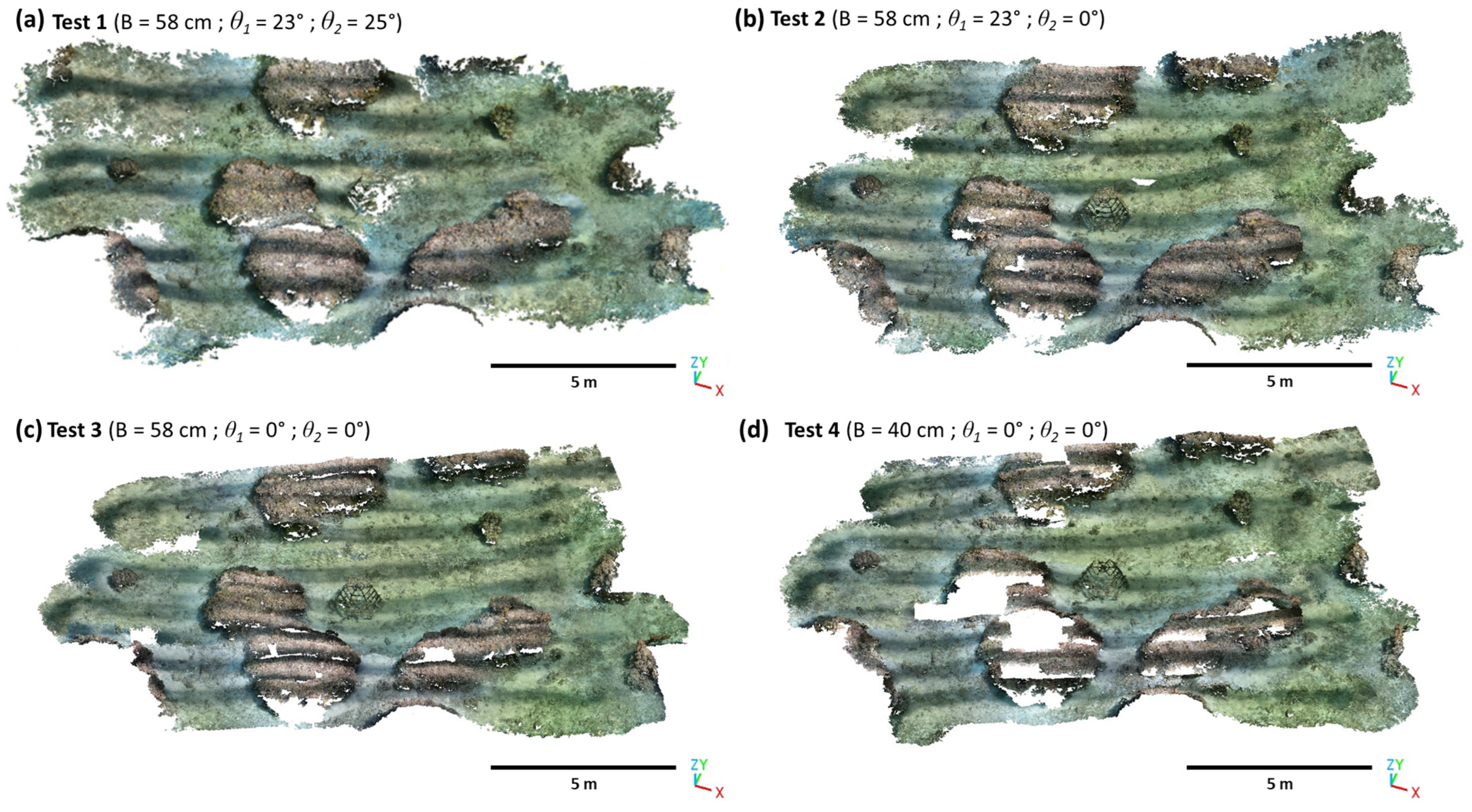
- In the Hermitage reef flat: very shallow depths (around 40 cm to 1 m of water) and sudden variations in bathymetry due to coral heads were expected. In this challenging case, various configurations were tested (Tests 1 to 4 in Table 1). The speed of the platform was around 1.5 km/h (higher than in the previous case, mainly because of the current).
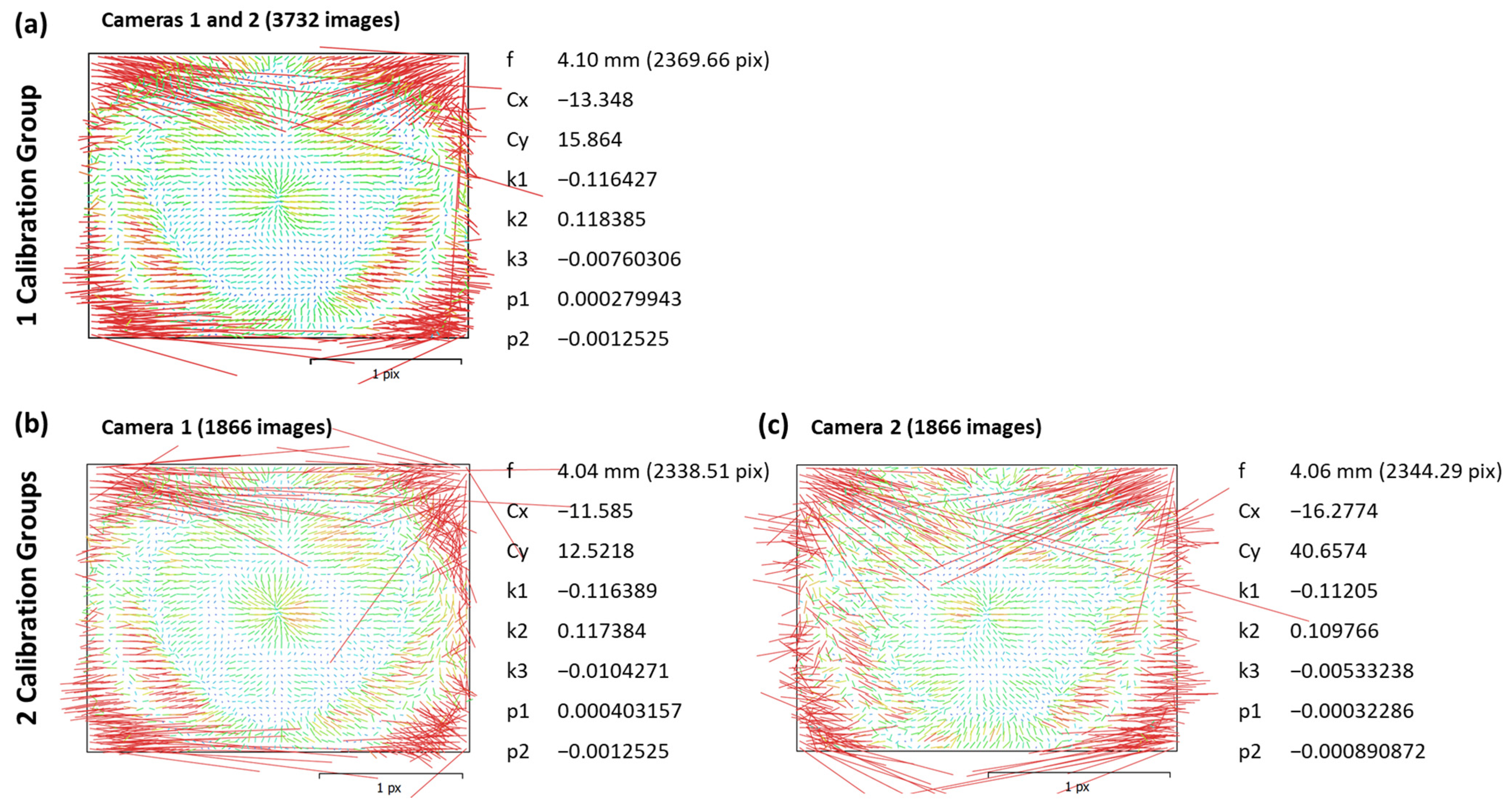
- The first processing step consists of “aligning the images” by bundle adjustment. A SIFT (Scale Invariant Feature Transform) algorithm [55] performed the detection and matching of homologous keypoints in overlapping photographs. From the resulting tie points, the camera external parameters (position, orientation) were computed and/or optimized by aerotriangulation (and the collinearity equations), for both Camera 1 and Camera 2. In Agisoft Metashape, the accuracy was set to “high”, which means that the software works with the photos of the original size. Keypoint limit and tie point limit were set to their default values. The ‘Reference preselection’ was set to ‘Source’. The ‘Guided image matching’ was selected.
- Camera internal parameters are refined by self-calibration, on the basis of knowledge of the accurate position of the cameras and modelling the distortion of the lens with Brown’s distortion model [56]. For this ‘Camera Optimization’ step, the default parameters were kept in Agisoft Metashape.
- A georeferenced dense point cloud is then generated by dense image matching using the estimated camera external and internal parameters. For this step, in Metashape, the ‘Quality’ parameter was set to ‘High’ to obtain more detailed and accurate geometry; the depth filtering mode was set to ‘aggressive’ or ‘moderate’, depending on the level of detail to be preserved.
4. Results
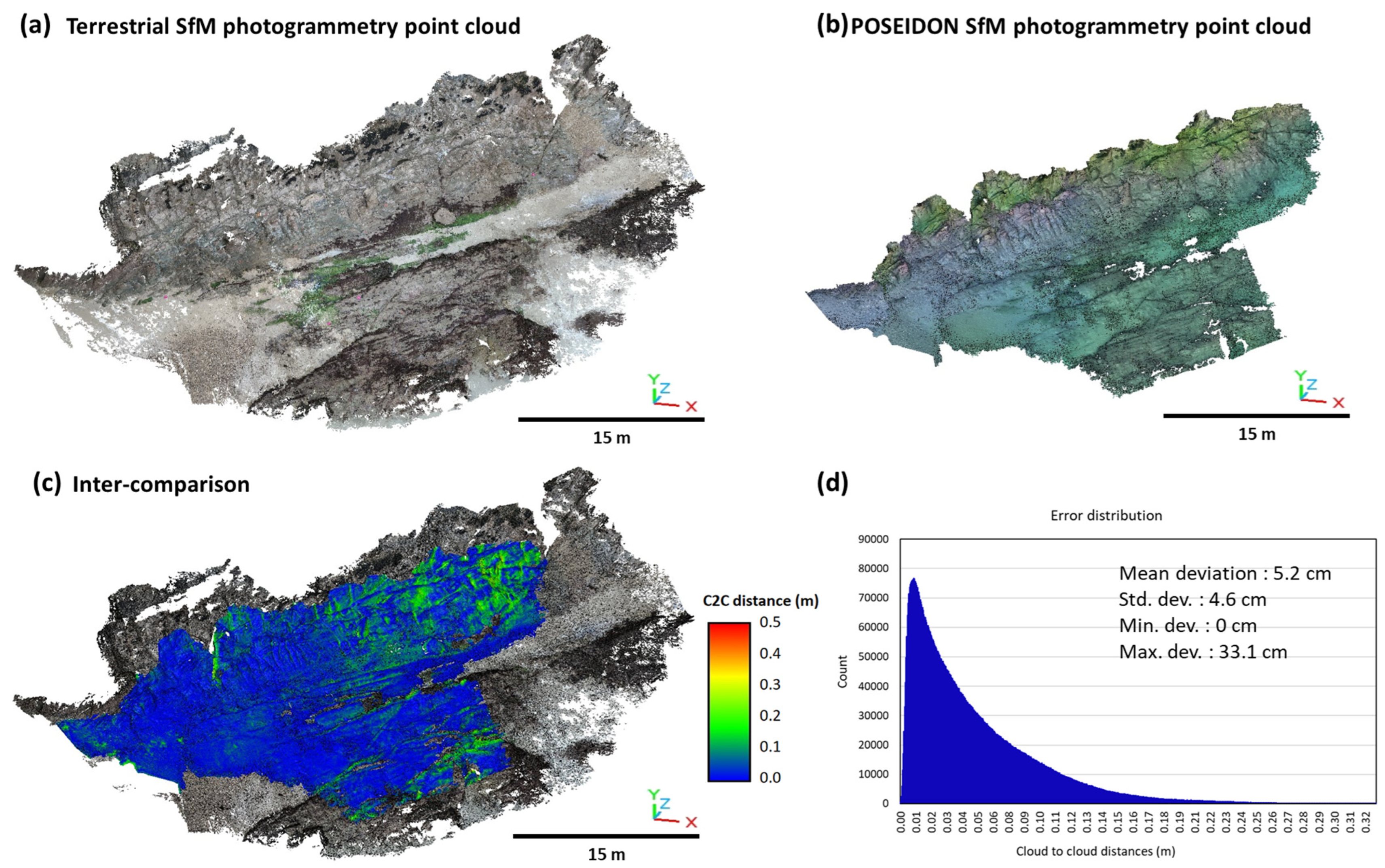
4.1. Dellec Bay
4.2. Hermitage Backreef Zone
5. Discussion
5.1. Main Benefits and Constraints on Using POSEIDON
5.2. POSEIDON Development Options
6. Conclusions
Author Contributions
Funding
Data Availability Statement
Acknowledgments
Conflicts of Interest
References
- Collins, W.T.; Galloway, J.L. Seabed Classification with Multibeam Bathymetry. Sea Technol. 1998, 39, 45–50. [Google Scholar]
- Pandian, P.K.; Ruscoe, J.P.; Shields, M.; Side, J.C.; Harris, R.E.; Kerr, S.A.; Bullen, C.R. Seabed Habitat Mapping Techniques: An Overview of the Performance of Various Systems. Mediterr. Mar. Sci. 2009, 10, 29. [Google Scholar] [CrossRef]
- Borrelli, M.; Smith, T.L.; Mague, S.T. Vessel-Based, Shallow Water Mapping with a Phase-Measuring Sidescan Sonar. Estuaries Coasts 2022, 45, 961–979. [Google Scholar] [CrossRef]
- Allouis, T.; Bailly, J.-S.; Pastol, Y.; Le Roux, C. Comparison of LiDAR Waveform Processing Methods for Very Shallow Water Bathymetry Using Raman, near-Infrared and Green Signals. Earth Surf. Process. Landf. 2010, 35, 640–650. [Google Scholar] [CrossRef]
- Yang, F.; Qi, C.; Su, D.; Ding, S.; He, Y.; Ma, Y. An Airborne LiDAR Bathymetric Waveform Decomposition Method in Very Shallow Water: A Case Study around Yuanzhi Island in the South China Sea. Int. J. Appl. Earth Obs. Geoinf. 2022, 109, 102788. [Google Scholar] [CrossRef]
- Szafarczyk, A.; Toś, C. The Use of Green Laser in LiDAR Bathymetry: State of the Art and Recent Advancements. Sensors 2022, 23, 292. [Google Scholar] [CrossRef] [PubMed]
- Sous, D.; Bouchette, F.; Doerflinger, E.; Meulé, S.; Certain, R.; Toulemonde, G.; Dubarbier, B.; Salvat, B. On the Small-scale Fractal Geometrical Structure of a Living Coral Reef Barrier. Earth Surf. Process. Landf. 2020, 45, 3042–3054. [Google Scholar] [CrossRef]
- Fritsch, N.; Fromant, G.; Hurther, D.; Caceres, I. Coarse Sand Transport Processes in the Ripple Vortex Regime under Asymmetric Nearshore Waves. JGR-Ocean, 2023; in press. [Google Scholar]
- Raoult, V.; David, P.A.; Dupont, S.F.; Mathewson, C.P.; O’Neill, S.J.; Powell, N.N.; Williamson, J.E. GoPros™ as an Underwater Photogrammetry Tool for Citizen Science. PeerJ 2016, 4, e1960. [Google Scholar] [CrossRef]
- Jaud, M.; Kervot, M.; Delacourt, C.; Bertin, S. Potential of Smartphone SfM Photogrammetry to Measure Coastal Morphodynamics. Remote Sens. 2019, 11, 2242. [Google Scholar] [CrossRef]
- Fabris, M.; Fontana Granotto, P.; Monego, M. Expeditious Low-Cost SfM Photogrammetry and a TLS Survey for the Structural Analysis of Illasi Castle (Italy). Drones 2023, 7, 101. [Google Scholar] [CrossRef]
- Girod, L.; Nuth, C.; Kääb, A.; Etzelmüller, B.; Kohler, J. Terrain Changes from Images Acquired on Opportunistic Flights by SfM Photogrammetry. Cryosphere 2017, 11, 827–840. [Google Scholar] [CrossRef]
- Bryson, M.; Duce, S.; Harris, D.; Webster, J.M.; Thompson, A.; Vila-Concejo, A.; Williams, S.B. Geomorphic Changes of a Coral Shingle Cay Measured Using Kite Aerial Photography. Geomorphology 2016, 270, 1–8. [Google Scholar] [CrossRef]
- Feurer, D.; Planchon, O.; El Maaoui, M.A.; Ben Slimane, A.; Boussema, M.R.; Pierrot-Deseilligny, M.; Raclot, D. Using Kites for 3-D Mapping of Gullies at Decimetre-Resolution over Several Square Kilometres: A Case Study on the Kamech Catchment, Tunisia. Nat. Hazards Earth Syst. Sci. 2018, 18, 1567–1582. [Google Scholar] [CrossRef]
- Jaud, M.; Delacourt, C.; Le Dantec, N.; Allemand, P.; Ammann, J.; Grandjean, P.; Nouaille, H.; Prunier, C.; Cuq, V.; Augereau, E.; et al. Diachronic UAV Photogrammetry of a Sandy Beach in Brittany (France) for a Long-Term Coastal Observatory. ISPRS Int. J. Geo-Inf. 2019, 8, 267. [Google Scholar] [CrossRef]
- James, M.R.; Robson, S. Straightforward Reconstruction of 3D Surfaces and Topography with a Camera: Accuracy and Geoscience Application: 3D Surfaces and Topography with a Camera. J. Geophys. Res. Earth Surf. 2012, 117, 03017. [Google Scholar] [CrossRef]
- Bessin, Z.; Jaud, M.; Letortu, P.; Vassilakis, E.; Evelpidou, N.; Costa, S.; Delacourt, C. Smartphone Structure-from-Motion Photogrammetry from a Boat for Coastal Cliff Face Monitoring Compared with Pléiades Tri-Stereoscopic Imagery and Unmanned Aerial System Imagery. Remote Sens. 2023, 15, 3824. [Google Scholar] [CrossRef]
- Wright, A.E.; Conlin, D.L.; Shope, S.M. Assessing the Accuracy of Underwater Photogrammetry for Archaeology: A Comparison of Structure from Motion Photogrammetry and Real Time Kinematic Survey at the East Key Construction Wreck. J. Mar. Sci. Eng. 2020, 8, 849. [Google Scholar] [CrossRef]
- Urbina-Barreto, I.; Garnier, R.; Elise, S.; Pinel, R.; Dumas, P.; Mahamadaly, V.; Facon, M.; Bureau, S.; Peignon, C.; Quod, J.-P.; et al. Which Method for Which Purpose? A Comparison of Line Intercept Transect and Underwater Photogrammetry Methods for Coral Reef Surveys. Front. Mar. Sci. 2021, 8, 636902. [Google Scholar] [CrossRef]
- Ventura, D.; Mancini, G.; Casoli, E.; Pace, D.S.; Lasinio, G.J.; Belluscio, A.; Ardizzone, G. Seagrass Restoration Monitoring and Shallow-Water Benthic Habitat Mapping through a Photogrammetry-Based Protocol. J. Environ. Manag. 2022, 304, 114262. [Google Scholar] [CrossRef]
- Del Savio, A.A.; Luna Torres, A.; Vergara Olivera, M.A.; Llimpe Rojas, S.R.; Urday Ibarra, G.T.; Neckel, A. Using UAVs and Photogrammetry in Bathymetric Surveys in Shallow Waters. Appl. Sci. 2023, 13, 3420. [Google Scholar] [CrossRef]
- He, J.; Lin, J.; Ma, M.; Liao, X. Mapping Topo-Bathymetry of Transparent Tufa Lakes Using UAV-Based Photogrammetry and RGB Imagery. Geomorphology 2021, 389, 107832. [Google Scholar] [CrossRef]
- Dietrich, J.T. Bathymetric Structure-from-Motion: Extracting Shallow Stream Bathymetry from Multi-View Stereo Photogrammetry: Bathymetric Structure-From-Motion. Earth Surf. Process. Landf. 2017, 42, 355–364. [Google Scholar] [CrossRef]
- Burns, J.H.R.; Delparte, D.; Gates, R.D.; Takabayashi, M. Utilizing Underwater Three-Dimensional Modeling to Enhance Ecological and Biological Studies of Coral Reefs. Int. Arch. Photogramm. Remote Sens. Spat. Inf. Sci. 2015, XL-5/W5, 61–66. [Google Scholar] [CrossRef]
- Urbina-Barreto, I. New Quantitative Indices from 3D Modeling by Photogrammetry to Monitor Coral Reef Environments. Ph.D. Thesis, Université de la Réunion, Saint-Denis, France, 2020. [Google Scholar]
- David, C.G.; Kohl, N.; Casella, E.; Rovere, A.; Ballesteros, P.; Schlurmann, T. Structure-from-Motion on Shallow Reefs and Beaches: Potential and Limitations of Consumer-Grade Drones to Reconstruct Topography and Bathymetry. Coral Reefs 2021, 40, 835–851. [Google Scholar] [CrossRef]
- Casella, E.; Lewin, P.; Ghilardi, M.; Rovere, A.; Bejarano, S. Assessing the Relative Accuracy of Coral Heights Reconstructed from Drones and Structure from Motion Photogrammetry on Coral Reefs. Coral Reefs 2022, 41, 869–875. [Google Scholar] [CrossRef]
- Green, J.; Gainsford, M. Evaluation of Underwater Surveying Techniques. Int. J. Naut. Archaeol. 2003, 32, 252–261. [Google Scholar] [CrossRef]
- Costa, E.; Guerra, F.; Vernier, P. Self-Assembled ROV and Photogrammetric Surveys with Low Cost Techniques. Int. Arch. Photogramm. Remote Sens. Spat. Inf. Sci. 2018, XLII-2, 275–279. [Google Scholar] [CrossRef]
- Price, D.M.; Robert, K.; Callaway, A.; Lo Lacono, C.; Hall, R.A.; Huvenne, V.A.I. Using 3D Photogrammetry from ROV Video to Quantify Cold-Water Coral Reef Structural Complexity and Investigate Its Influence on Biodiversity and Community Assemblage. Coral Reefs 2019, 38, 1007–1021. [Google Scholar] [CrossRef]
- Menna, F.; Nocerino, E.; Nawaf, M.M.; Seinturier, J.; Torresani, A.; Drap, P.; Remondino, F.; Chemisky, B. Towards Real-Time Underwater Photogrammetry for Subsea Metrology Applications. In Proceedings of the OCEANS 2019-Marseille, Marseille, France, 17–20 June 2019; IEEE: Marseille, France, 2019; pp. 1–10. [Google Scholar]
- Teague, J.; Scott, T. Underwater Photogrammetry and 3D Reconstruction of Submerged Objects in Shallow Environments by ROV and Underwater GPS. J. Mar. Sci. Res. Technol. 2017. [Google Scholar]
- Wu, Y.; Ta, X.; Xiao, R.; Wei, Y.; An, D.; Li, D. Survey of Underwater Robot Positioning Navigation. Appl. Ocean Res. 2019, 90, 101845. [Google Scholar] [CrossRef]
- Luo, Q.; Yan, X.; Ju, C.; Chen, Y.; Luo, Z. An Ultra-Short Baseline Underwater Positioning System with Kalman Filtering. Sensors 2020, 21, 143. [Google Scholar] [CrossRef] [PubMed]
- Leon, J.X.; Roelfsema, C.M.; Saunders, M.I.; Phinn, S.R. Measuring Coral Reef Terrain Roughness Using ‘Structure-from-Motion’ Close-Range Photogrammetry. Geomorphology 2015, 242, 21–28. [Google Scholar] [CrossRef]
- Ventura, D.; Dubois, S.F.; Bonifazi, A.; Jona Lasinio, G.; Seminara, M.; Gravina, M.F.; Ardizzone, G. Integration of Close-range Underwater Photogrammetry with Inspection and Mesh Processing Software: A Novel Approach for Quantifying Ecological Dynamics of Temperate Biogenic Reefs. Remote Sens. Ecol. Conserv. 2021, 7, 169–186. [Google Scholar] [CrossRef]
- Raber, G.T.; Schill, S.R. Reef Rover: A Low-Cost Small Autonomous Unmanned Surface Vehicle (USV) for Mapping and Monitoring Coral Reefs. Drones 2019, 3, 38. [Google Scholar] [CrossRef]
- Bonhommeau, S. Projet PLANCHA. Available online: https://ocean-indien.ifremer.fr/en/Projects/Technological-innovations/PLANCHA-2021-2023 (accessed on 3 July 2023).
- InfoClimat. Climatologie Mensuelle/Observations-Météo/Archives, in Brest-Guipavas Station and Le Port station. Available online: https://www.infoclimat.fr/ (accessed on 5 July 2023).
- Cordier, E.; Lézé, J.; Join, J.-L. Natural Tidal Processes Modified by the Existence of Fringing Reef on La Reunion Island (Western Indian Ocean): Impact on the Relative Sea Level Variations. Cont. Shelf Res. 2013, 55, 119–128. [Google Scholar] [CrossRef]
- Westoby, M.J.; Brasington, J.; Glasser, N.F.; Hambrey, M.J.; Reynolds, J.M. ‘Structure-from-Motion’ Photogrammetry: A Low-Cost, Effective Tool for Geoscience Applications. Geomorphology 2012, 179, 300–314. [Google Scholar] [CrossRef]
- Javernick, L.; Brasington, J.; Caruso, B. Modeling the Topography of Shallow Braided Rivers Using Structure-from-Motion Photogrammetry. Geomorphology 2014, 213, 166–182. [Google Scholar] [CrossRef]
- Carrivick, J.; Smith, M.; Quincey, D. Structure from Motion in the Geosciences; Wiley, Blackwell: Chichester, UK; Ames, IA, USA, 2016; ISBN 978-1-118-89584-9. [Google Scholar]
- Eltner, A.; Sofia, G. Structure from Motion Photogrammetric Technique. In Developments in Earth Surface Processes; Elsevier: Amsterdam, The Netherlands, 2020; Volume 23, pp. 1–24. ISBN 978-0-444-64177-9. [Google Scholar]
- Elhadary, A.; Rabah, M.; Ghanim, E.; Mohie, R.; Taha, A. The Influence of Flight Height and Overlap on UAV Imagery over Featureless Surfaces and Constructing Formulas Predicting the Geometrical Accuracy. NRIAG J. Astron. Geophys. 2022, 11, 210–223. [Google Scholar] [CrossRef]
- Dai, F.; Feng, Y.; Hough, R. Photogrammetric Error Sources and Impacts on Modeling and Surveying in Construction Engineering Applications. Vis. Eng. 2014, 2, 2. [Google Scholar] [CrossRef]
- Neyer, F.; Nocerino, E.; Gruen, A. Image Quality Improvements in low-cost underwater photogrammetry. Int. Arch. Photogramm. Remote Sens. Spatial Inf. Sci. 2019, XLII-2/W10, 135–142. [Google Scholar] [CrossRef]
- James, M.R.; Robson, S. Mitigating Systematic Error in Topographic Models Derived from UAV and Ground-Based Image Networks: Mitigating Systematic Error in Topographic Models. Earth Surf. Process. Landf. 2014, 39, 1413–1420. [Google Scholar] [CrossRef]
- Jaud, M.; Passot, S.; Allemand, P.; Le Dantec, N.; Grandjean, P.; Delacourt, C. Suggestions to Limit Geometric Distortions in the Reconstruction of Linear Coastal Landforms by SfM Photogrammetry with PhotoScan® and MicMac® for UAV Surveys with Restricted GCPs Pattern. Drones 2019, 3, 2. [Google Scholar] [CrossRef]
- Jaud, M.; Bertin, S.; Beauverger, M.; Augereau, E.; Delacourt, C. RTK GNSS-Assisted Terrestrial SfM Photogrammetry without GCP: Application to Coastal Morphodynamics Monitoring. Remote Sens. 2020, 12, 1889. [Google Scholar] [CrossRef]
- Štroner, M.; Urban, R.; Seidl, J.; Reindl, T.; Brouček, J. Photogrammetry Using UAV-Mounted GNSS RTK: Georeferencing Strategies without GCPs. Remote Sens. 2021, 13, 1336. [Google Scholar] [CrossRef]
- Bertin, S.; Floc’h, F.; Le Dantec, N.; Jaud, M.; Cancouët, R.; Franzetti, M.; Cuq, V.; Prunier, C.; Ammann, J.; Augereau, E.; et al. A Long-Term Dataset of Topography and Nearshore Bathymetry at the Macrotidal Pocket Beach of Porsmilin, France. Sci. Data 2022, 9, 79. [Google Scholar] [CrossRef] [PubMed]
- Le Réseau Centipède RTK. Available online: https://docs.centipede.fr/ (accessed on 4 December 2023).
- Delsol, S. POSEIDON-Processing 2023. Available online: https://github.com/sDelsol (accessed on 4 December 2023).
- Lowe, D.G. Distinctive Image Features from Scale-Invariant Keypoints. Int. J. Comput. Vis. 2004, 60, 91–110. [Google Scholar] [CrossRef]
- Agisoft Metashape User Manual-Professional Edition, Version 1.7; Agisoft LLC: Saint Petersburg, Russia, 2021. Available online: https://www.agisoft.com/pdf/metashape-pro_1_7_en.pdf (accessed on 29 September 2023).
- Tournadre, V.; Pierrot-Deseilligny, M.; Faure, P.H. UAV LINEAR PHOTOGRAMMETRY. Int. Arch. Photogramm. Remote Sens. Spat. Inf. Sci. 2015, XL-3/W3, 327–333. [Google Scholar] [CrossRef]
- Luhmann, T.; Fraser, C.; Maas, H.-G. Sensor Modelling and Camera Calibration for Close-Range Photogrammetry. ISPRS J. Photogramm. Remote Sens. 2016, 115, 37–46. [Google Scholar] [CrossRef]
- Nesbit, P.; Hugenholtz, C. Enhancing UAV–SfM 3D Model Accuracy in High-Relief Landscapes by Incorporating Oblique Images. Remote Sens. 2019, 11, 239. [Google Scholar] [CrossRef]
- Huang, W.; Jiang, S.; Jiang, W. Camera Self-Calibration with GNSS Constrained Bundle Adjustment for Weakly Structured Long Corridor UAV Images. Remote Sens. 2021, 13, 4222. [Google Scholar] [CrossRef]


| Configuration | Baseline | Camera Orientation (±2°) | Constraints on Trajectory | |
|---|---|---|---|---|
| Test 1 |  | 58 cm | θ1 = 23° θ2 = 25° | Inter-transect distance: 0.9–1 m Return transects: yes |
| Test 2 | 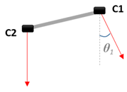 | 58 cm | θ1 = 23° θ2 = 0° (nadir) | Inter-transect distance: 0.9–1 m Return transects: yes |
| Test 3 | 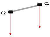 | 58 cm | θ1 = 0° (nadir) θ2 = 0° (nadir) | Inter-transect distance: 0.9–1 m Return transects: no |
| Test 4 | 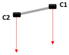 | 40 cm | θ1 = 0° (nadir) θ2 = 0° (nadir) | Inter-transect distance: 0.9–1 m Return transects: no |
| Agisoft Metashape Processing Step | Used Parameters |
|---|---|
| Image alignment | Accuracy: High Generic preselection Reference preselection: Source Key point limit: 40,000 Tie point limit: 10,000 Exclude stationary tie points Guided image matching |
| Optimize cameras | Default parameters |
| Build dense point cloud | Quality: High Depth filtering: Aggressive/Moderate (depending on the environment) Calculate point colours Calculate point confidence |
| Number of Photos Aligned | Number of Points | Modelled Surface Area | Native Mean Point Density | |
|---|---|---|---|---|
| Test 1 | 2230 of 2863 (78%) | 508,103,069 | 230 m2 | 2.2 × 10⁶ pts/m2 |
| Test 2 | 2862 of 3732 (77%) | 588,004,876 | 210 m2 | 2.8 × 10⁶ pts/m2 |
| Test 3 | 2924 of 3524 (84%) | 492,951,386 | 156 m2 | 3.2 × 10⁶ pts/m2 |
| Test 4 | 2140 of 2630 (81%) | 436,343,004 | 148 m2 | 2.9 × 10⁶ pts/m2 |
| Point Cloud Compared to Test 2 | Mean Distance (cm) | Standard Deviation (cm) |
|---|---|---|
| Test 1 | −1.7 | 6.3 |
| Test 3 | 1.3 | 6.2 |
| Test 4 | 0.3 | 7.8 |
Disclaimer/Publisher’s Note: The statements, opinions and data contained in all publications are solely those of the individual author(s) and contributor(s) and not of MDPI and/or the editor(s). MDPI and/or the editor(s) disclaim responsibility for any injury to people or property resulting from any ideas, methods, instructions or products referred to in the content. |
© 2023 by the authors. Licensee MDPI, Basel, Switzerland. This article is an open access article distributed under the terms and conditions of the Creative Commons Attribution (CC BY) license (https://creativecommons.org/licenses/by/4.0/).
Share and Cite
Jaud, M.; Delsol, S.; Urbina-Barreto, I.; Augereau, E.; Cordier, E.; Guilhaumon, F.; Le Dantec, N.; Floc’h, F.; Delacourt, C. Low-Tech and Low-Cost System for High-Resolution Underwater RTK Photogrammetry in Coastal Shallow Waters. Remote Sens. 2024, 16, 20. https://doi.org/10.3390/rs16010020
Jaud M, Delsol S, Urbina-Barreto I, Augereau E, Cordier E, Guilhaumon F, Le Dantec N, Floc’h F, Delacourt C. Low-Tech and Low-Cost System for High-Resolution Underwater RTK Photogrammetry in Coastal Shallow Waters. Remote Sensing. 2024; 16(1):20. https://doi.org/10.3390/rs16010020
Chicago/Turabian StyleJaud, Marion, Simon Delsol, Isabel Urbina-Barreto, Emmanuel Augereau, Emmanuel Cordier, François Guilhaumon, Nicolas Le Dantec, France Floc’h, and Christophe Delacourt. 2024. "Low-Tech and Low-Cost System for High-Resolution Underwater RTK Photogrammetry in Coastal Shallow Waters" Remote Sensing 16, no. 1: 20. https://doi.org/10.3390/rs16010020
APA StyleJaud, M., Delsol, S., Urbina-Barreto, I., Augereau, E., Cordier, E., Guilhaumon, F., Le Dantec, N., Floc’h, F., & Delacourt, C. (2024). Low-Tech and Low-Cost System for High-Resolution Underwater RTK Photogrammetry in Coastal Shallow Waters. Remote Sensing, 16(1), 20. https://doi.org/10.3390/rs16010020