Abstract
In recent years, deep learning methods utilizing convolutional neural networks have been extensively employed in hyperspectral image classification (HSI) applications. Nevertheless, while a substantial number of stacked 3D convolutions can indeed achieve high classification accuracy, they also introduce a significant number of parameters to the model, resulting in inefficiency. Furthermore, such intricate models often exhibit limited classification accuracy when confronted with restricted sample data, i.e., small sample problems. Therefore, we propose a spectral–spatial double-branch network (SSDBN) with an attention mechanism for HSI classification. The SSDBN is designed with two independent branches to extract spectral and spatial features, respectively, incorporating multi-scale 2D convolution modules, long short-term memory (LSTM), and an attention mechanism. The flexible use of 2D convolution, instead of 3D convolution, significantly reduces the model’s parameter count, while the effective spectral–spatial double-branch feature extraction method allows SSDBN to perform exceptionally well in handling small sample problems. When tested on 5%, 0.5%, and 5% of the Indian Pines, Pavia University, and Kennedy Space Center datasets, SSDBN achieved classification accuracies of 97.56%, 96.85%, and 98.68%, respectively. Additionally, we conducted a comparison of training and testing times, with results demonstrating the remarkable efficiency of SSDBN.
1. Introduction
Hyperspectral images (HSIs) typically encompass tens or even hundreds of bands with rich spatial and spectral information [1]. Hyperspectral techniques can be used for hyperspectral imaging [2]. HSI classification refers to the process of categorizing land cover or objects within a scene using hyperspectral image data. It represents a critical task in HSI analysis and it finds a wide array of applications in fields such as vegetation cover monitoring [3], change detection [4], and atmospheric environmental studies [5].
Considerable attention has been paid to the study of HSI classification. Many effective methods have been devised to address the HSI classification task. Early methods, in particular, include traditional approaches like support vector machine (SVM) [6], k-nearest neighbor [7], and multinomial logistic regression [8]. These methods primarily concentrate on the spectral information of HSIs while overlooking the high spatial correlation within them. This oversight results in the loss of valuable spatial information, consequently limiting the classification accuracy. To utilize both spectral and spatial information, Huo et al. [9] successfully extracted both spectral and spatial details from HSIs. This was achieved by incorporating SVM and Gabor filters. Fang et al. [10] applied a method of clustering HSIs into numerous superpixels. This effectively leverages both spectral and spatial information through multiple kernels. Tarabalka et al. [11] applied probabilistic SVM for pixel-by-pixel HSI classification. They improved results by incorporating spatial contextual information into the classification process through Markov random field regularization. While these methods enhance classification accuracy, they all rely on manually designed feature extraction techniques. These techniques involve complex modeling procedures, limited feature expression capability, and weak generalization capability. This makes them insufficient to meet higher classification requirements.
In recent years, there have been continuous breakthroughs in deep learning in various fields such as target detection [12], image classification [13], and natural language processing [14]. This has made the utilization of deep learning methods to extract deep features from HSIs a viable option. A large number of research results show that deep learning methods are better at extracting higher-level features than traditional methods. These deep features can characterize more complex and abstract structural information, resulting in a significant enhancement of HSI classification accuracy. For example, Chen et al. [15] proposed a stacked autoencoder to obtain useful high-level features for HSI. Li et al. [16] introduced deep belief networks (DBN) to HSI feature extraction and classification. They employed the restricted Boltzmann machine as the hierarchical framework for DBN and the results proved that the DBN method can achieve excellent performance. However, the above methods flatten the input into vectors in the spatial feature extraction stage, which can lead to some loss of spatial information.
To address this problem, convolutional neural network (CNN)-based approaches were applied to the field of HSI classification [17,18,19]. Hu et al. [17] used 1D CNNs for HSI classification. They represented the hundreds of bands of HSI as one-dimensional vectors, focusing solely on spectral features and neglecting spatial features. Makantasis et al. [18] applied 2D CNNs for spatial feature extraction in HSI. They combined principal component analysis and multilayer perceptron to construct high-level features encoding both spectral and spatial information. Chen et al. [19] used 3D CNNs to construct a finite element model. They addressed the common problem of imbalance between finite samples of HSIs and high-dimensional features. This was achieved through the use of regularization and dropout to avoid overfitting. Finally, their approach effectively extracted spectral and spatial features of HSIs. Roy et al. [20] proposed a hybrid spectral CNN (HybridSN), where 3D CNNs extract joint spectral–spatial features of spectral bands and 2D CNNs further learn the spatial representation at the abstraction level. The results demonstrated that the hybrid CNN performed better than 3D CNN or 2D CNN alone for classification. He et al. [21] proposed a multi-scale 3D CNN (M3D-CNN) for HSI classification. The model jointly learned 2D multi-scale spatial features and 1D spectral features from HSI in an end-to-end manner. This approach led to advanced classification results. To mitigate the decline of deep learning accuracy, Zhong et al. [22] designed a spectral–spatial residual network (SSRN). The SSRN incorporates spectral and spatial residual blocks, extracting rich spectral features and spatial contextual discriminative features from HSI. The residual blocks are connected to other 3D convolutional layers through constant mapping, which alleviates the training difficulty of the network. Mei et al. [23] proposes a spectral–spatial attention network for hyperspectral image classification. It introduces recurrent neural network (RNN) and CNN with attention mechanisms. The attention-equipped RNN captures spectral correlations within a continuous spectrum. Meanwhile, the attention-equipped CNN focuses on saliency features and spatial relationships among neighboring pixels in the spatial dimension. Li et al. [24] applied a band attention module and a spatial attention module to alleviate the effects of redundant bands and interfering pixels. They extracted spectral and spatial features through multi-scale convolution. Ma et al. [25] proposed a two-branch multi-attention mechanism network (DBMA). The network utilizes attention mechanisms to refine the feature map, resulting in optimal classification results. Attention mechanisms are increasingly employed in HSI classification tasks. In [26], Xu et al. combined shallow and deep features using a multi-level feature fusion strategy. This approach enabled the model to leverage multi-scale information and achieve better adaptability for HSI classification. As seen, the models used in HSI classification are becoming increasingly complex and parameterized. They achieve high accuracy with sufficient samples but may exhibit a less-than-optimal performance in the presence of small sample problems.
To address the above challenges, we propose the spectral–spatial double-branch network (SSDBN) with attention mechanisms for HSI classification. This network consists of two independent branches—one for spectral and the other for spatial feature extraction. Additionally, we utilize advanced spectral attention and spatial attention modules to obtain classification results. On the spectral branch, we employ 1D convolution and long short-term memory (LSTM) for extracting spectral features. Simultaneously, on the spatial branch, we utilize serial multi-scale 2D convolution for extracting spatial features. The paper’s main contributions are as follows:
(1) We propose the spectral–spatial double-branch network (SSDBN) for HSI classification. This network is designed as an end-to-end HSI classification system that incorporates attention mechanisms, LSTM, and multi-scale 2D convolution. It discards multi-scale 3D convolution and serially employs multiple multi-scale 2D convolution modules. Moreover, the network fuses the outputs of multi-level multi-scale modules to extract spatial features and it utilizes the spectral sequence processing module (SSPM) and LSTM modules to extract spectral features. The whole network can maintain an excellent classification performance while significantly reducing the number of parameters;
(2) We invoke state-of-the-art lightweight spectral and spatial attention modules, resulting in negligible overhead and a simple yet efficient enough structure;
(3) The proposed algorithm attains superior classification results on three public datasets with small sample data, and the time for training and testing are also ahead of other deep learning algorithms.
The rest of the paper is organized as follows: in Section 2, we describe the detailed structure of the proposed SSDBN. In Section 3, we introduce the three datasets used in the experiments. In Section 4 and Section 5, we provide and analyze the results of the comparison and ablation experiments, respectively. Finally, we conclude the full paper and suggest directions for future work in Section 6.
2. Methodology
The proposed overall framework of the SSDBN is shown in Figure 1. HSI can be viewed as a 3D cube of shape H × W × B, where H, W, and B represent the height, width, and number of bands, respectively. First, the HSI is cut into 3D cubes of 9 × 9 × B. Then, the 3D cubes are divided into training, validation, and testing sets according to the set scale. The training set is employed to fit the sample data and train different models, the validation set is utilized to select the optimal model, and the performance of the model is evaluated by the testing set in the prediction phase. To determine whether the model converges in the training phase, the difference between the predicted and true values is usually measured using a cross-entropy loss function, which is defined as:
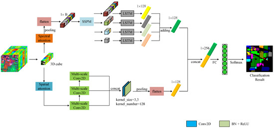
Figure 1.
Architecture of the proposed model.
These 3D cubes are subsequently directed to the spectral and spatial branches, then the spectral and spatial feature maps obtained, respectively, are fused for classification. The SSDBN mainly includes the following modules: multi-scale 2D convolution, SSPM, LSTM, and an attention mechanism. The multi-scale 2D convolution module consists of four parallel 2D convolution kernels for extracting spatial information and three serial multi-scale 2D convolution modules for multi-layer feature fusion, to achieve full extraction of spatial features. The SSPM module processes the spectral sequences before input to the LSTM to enhance the performance of the LSTM layer. The LSTM is employed to capture spectral features from four spectral subsequences, and the attention mechanism serves to enhance the classification accuracy and speed up the model fitting. Each module is elaborated upon below.
2.1. RNN and LSTM
RNNs [27] perform the same task for each element in a sequence, and the output element depends on the previous element or state. Due to their remarkable capacity for encoding contextual information, RNNs have found extensive application in addressing sequence classification problems [28].
The structure diagram of an RNN is depicted in Figure 2. When provided with a set of sequences, the computation of a recurrent neural network can be represented by the following equations:
where b and c denote the bias vectors. W, U, and V are the weight matrices. , , and are the input, hidden, and output values at moment t, respectively. is the activation function and, in general, the function is chosen.
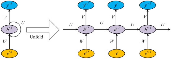
Figure 2.
Architecture of an RNN.
For the classification task, by adding the activation function, the final predicted model output can be obtained as:
where is the activation function, typically .
The loss function of RNN is usually chosen as cross entropy [29], and the loss function of the RNN model at moment t can be written as:
where and denote the label and predicted label of the ith data at moment t, respectively. N represents the number of input samples.
Then, taking into account all moments t, the loss function is defined as:
Since the RNN model is related to a time series, its parameters are optimized by the backpropagation through time, rather than using the back-propagation algorithm directly.
However, RNNs inevitably face the issue of gradient disappearance or explosion during backpropagation, so it is difficult to handle long sequences of data. To address this thorny problem, ref. [30] proposed the LSTM, which can avoid the gradient vanishing of traditional RNN, addresses the issue of long dependencies in RNNs, and is widely applied to various tasks, such as natural language processing [31] and financial market change prediction [32]. The general structure of LSTM is depicted in Figure 3.
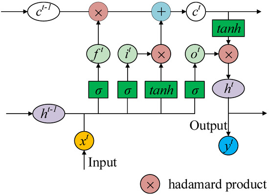
Figure 3.
Overall structure of an LSTM model.
The LSTM adds a cell state c to preserve the long-term state and controls the long-term state c through these three gates that act as control switches: forget gate f, input gate i, and output gate o. The forget gate determines how much of the cell state from the previous moment is preserved to the current moment ; the information in the cell state is discarded selectively, which is determined by the value of the sigmoid function, with 0 indicating all discard and 1 indicating all retention. The input gate determines how much of the input to the network at the current moment is preserved to the cell state at the current moment , selectively recording the input information into the cell state, and the output gate controls how much of the cell state at the current moment is output to the current output value of LSTM. The forward propagation of one LSTM cell at time t is calculated as follows:
where , , , and are the corresponding weight matrices, and , , , and are bias vectors. is the sigmoid function with the expression and function values between 0 and 1, is the hyperbolic tangent function with the expression and function values between and 1, and * is the hadamard product, indicating pixelwise multiplication.
2.2. SSPM
LSTM can achieve satisfactory results in extracting contextual information between adjacent sequence data, but HSI usually has tens or even hundreds of consecutive and highly correlated bands, so directly inputting such complex spectral sequences into LSTM for feature extraction will often lead to unsatisfactory results. In our proposed method, a processing strategy combining 1D convolution and average pooling is used to process the spectral sequences into four subsequences of different sizes by SSPM before inputting them into the LSTM module, which can extract useful spectral features in the LSTM module to compensate for its lack of performance and also makes the sequences shorter, reducing the time cost of the whole model. The illustration of SSPM is shown in Figure 4.
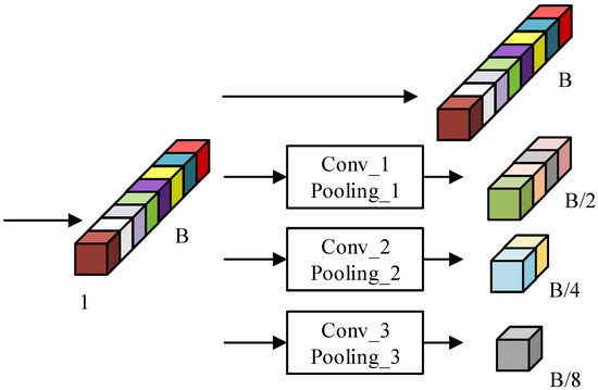
Figure 4.
Illustration of SSPM. The spectral sequence of size B is processed through four paths into four subsequences of size B, B/2, B/4, and B/8, where the subsequence of size B is identical to the original spectral sequence. Conv_1, Conv_2, and Conv_3 are all 1D convolutions with kernel_number = 1 and kernel_ size = 3. Pooling_1, Pooling_2 and Pooling_3 are 1D average pooling layers with kernel_sizes of 2, 4, and 8 and strides of 2, 4, and 8, respectively.
2.3. Multi-Scale 2D Convolution
Multi-scale convolution involves utilizing convolution kernels of various sizes simultaneously to learn multi-scale information [33]. The multi-scale information can be applied to address relevant classification problems because of the rich contextual information in the multi-scale structure [34]. In the HSI classification problem, it is currently popular to use multi-scale 3D convolutional blocks to build HSI classification network models and obtain excellent classification results [35]. To decrease the number of parameters and build a more lightweight network, the multi-scale 2D convolutional module is proposed, which consists of four convolutional kernels of different sizes in parallel. The structure of the proposed multi-scale 2D convolution module is shown in Figure 5. Compared to 3D convolution, one key advantage of using 2D convolution is that it operates across bands without considering the pixel’s position in each band. This approach reduces the model’s parameter count, lowers computational complexity, and mitigates the risk of overfitting during training. For hyperspectral images with numerous bands, the effectiveness of 2D convolution in capturing spectral information is evident. Therefore, the design choice of employing 2D convolution instead of 3D convolution contributes to enhanced model efficiency, reduced computational load, and decreased model complexity while maintaining performance.
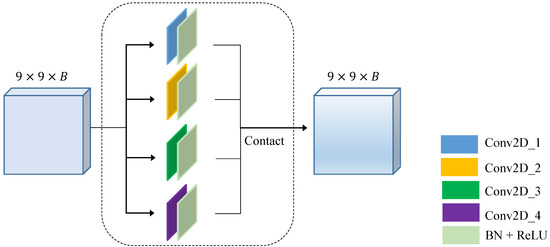
Figure 5.
Illustration of the multi-scale information extraction operation in this paper; the structure of the multi-scale 2D convolution module used is marked with a black dashed box.
The detailed parameter settings for this multi-scale 2D convolution module are shown in Table 1. We set several sets of parameters and, after testing, we chose this succinct set as it was sufficiently balanced for the accuracy and efficiency of the HSI classification task to meet our requirements for building a succinct network. In general, just one multi-scale 2D convolution module does not sufficiently extract the effective features of the HSI data, and we can choose to serialize several such modules. In this paper, the number of multi-scale modules is set to 3. The reason for choosing 3 will be demonstrated in the ablation experiments in later parts of the paper.

Table 1.
Parameters of multi-scale 2D convolution.
The input data of shape 9 × 9 × B is sent to the multi-scale convolution module. Since each multi-scale convolution performs the corresponding padding operation during feature extraction, the outputs of the four 2D convolutions are of equal size and, by concatenating these four outputs in the channel dimension, the resulting output size is equal to the input size, i.e., 9 × 9 × B.
2.4. Attention Mechanism
The significance of different spectral bands and spatial pixels in feature extraction varies, and the attention mechanism allows for a selective focus on regions abundant in feature information while considering non-essential areas less. For spectral classification, each pixel can be depicted as a continuous spectral profile containing rich spectral features, and we can use the channel attention mechanism to focus on the interrelationship between the bands of features. In spatial classification, the spatial attention mechanism can be used to increase the weights of compelling pixels and focus on the spatial relationships of features. These two modules are described in detail below.
2.4.1. Spectral Attention Module
Most existing research employs intricate attention modules to attain improved performance, and the increase in model complexity inevitably consumes a large number of computational resources. Wang et al. [36] proposed an effective channel attention (ECA) module that requires only a small number of additional parameters to deliver significant performance gains, which can effectively alleviate the tension between performance and complexity. The structure of this ECA module is shown in Figure 6.

Figure 6.
Diagram of the ECA module. The given input data will first go through global average pooling channel by channel to obtain the aggregated features. ECA will consider each channel and its k nearest neighbors to complete the computation of channel weights by fast 1D convolution. k is determined adaptively by mapping the channel dimension B.
Since the purpose of the ECA module is to properly capture local cross-channel information interactions, the approximate range of channel interaction information (i.e., k) needs to be determined. The optimal range of optimized information interactions (i.e., k) can be tuned manually for convolutional blocks with a different number of channels in various CNN architectures, but manual tuning by cross-validation can be computationally resource intensive. In recent studies, group convolution has been successfully used in CNN architectures [37] where high-dimensional (low-dimensional) channels are proportional to long-distance (short-distance) convolution for a fixed number of groups. Similarly, the coverage of cross-channel information interactions (i.e., k) should also be proportional to the number of channel dimensions B. In other words, there may be a mapping between k and B:
The simplest mapping is linear mapping. However, since linear functions have limitations in terms of representing certain relevant features and the channel dimension B is usually set to a power of 2. Therefore, a nonlinear mapping relationship can be represented by extending the linear function to an exponential function with a base of 2, i.e.:
Therefore, given the channel dimension B, the convolution kernel size k can be calculated smoothly by setting the values of and b.
2.4.2. Spatial Attention Module
The spatial attention mechanism aims to identify regions within the feature map that deserve focused attention. The convolutional block attention module (CBAM) [38] is a simple but efficient lightweight attention module. In the spatial dimension, given an feature F, two channel descriptions are first obtained by averaging pooling and max pooling in one channel dimension, respectively, and these two descriptions are stitched together by channels. Then, after a 2D convolution with the sigmoid activation function, the obtained weights are multiplied with the input features to obtain the adaptive refinement features. The spatial attention module used in the proposed method is schematically shown in Figure 7.

Figure 7.
Diagram of the CBAM module.
3. Datasets and Experimental Setting
3.1. Datasets
In this paper, we utilize three publicly available hyperspectral datasets—the Indian Pines (IP), Pavia University (UP), and Kennedy Space Center (KSC) datasets—to validate the accuracy and efficiency of the proposed method.
IP: This dataset was collected using the Airborne Visible Imaging Spectrometer (AVIRIS) in Northwest Indiana, USA, and consists of 200 spectral bands in the wavelength range of 0.4 µm to 2.5 µm after removal of the absorption band, with a spatial resolution of 20 m. Included in the dataset are 145 × 145 pixels and 16 land cover classes.
UP: This dataset was acquired at the University of Pavia in northern Italy with the Reflection Optical System Imaging Spectrometer (ROSIS) sensor. It comprises 103 spectral bands in the wavelength range of 0.43 µm to 0.86 µm with a spatial resolution of 1.3 m, the dataset contains 610 × 340 pixels and 9 land cover classes.
KSC: This dataset was collected by the AVIRIS sensor at the Kennedy Space Center, Florida, and comprises 224 bands and 512 × 340 pixels, with 176 bands remaining after water vapor noise removal. Additionally, it has a spectral coverage of 0.4 µm to 2.5 µm, with a spatial resolution of 18m and a total of 13 land coverage categories.
In the HSI classification task, the size of the training samples significantly impacts the classification accuracy. Generally, a larger training sample size leads to higher accuracy. However, more sample data also means increased time consumption and computational complexity. To assess the effectiveness of our model in addressing the small sample problem, we used minimal training and test sample sizes for each dataset in our experiments. For the Indian Pines and KSC datasets, we select 5% of the samples for training and 5% of the samples for validation. For the Pavia University dataset, with sufficient samples, we select only 0.5% of the samples for training and 0.5% of the samples for validation because of the very large number of training sample points. The training, validation, and test samples for the three datasets used for the experiments are listed in Table 2, Table 3 and Table 4, and the false-color images and ground truth maps are shown in Figure 8, Figure 9 and Figure 10.

Table 2.
The samples for each category of training, validation, and testing for the IP dataset.

Table 3.
The samples for each category of training, validation, and testing for the UP dataset.

Table 4.
The samples for each category of training, validation, and testing for the KSC dataset.

Figure 8.
Detailed information about the IP dataset. (a) False-color image. (b) Ground truth. (c) Labels illustration.
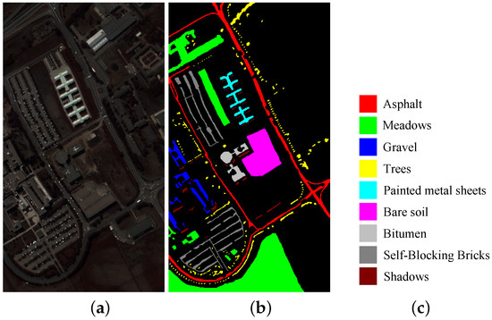
Figure 9.
Detailed information of the UP dataset. (a) False-color image. (b) Ground truth. (c) Labels illustration.

Figure 10.
Detailed information of the KSC dataset. (a) False-color image. (b) Ground truth. (c) Labels illustration.
3.2. Experimental Setting
To evaluate the proposed algorithm’s effectiveness, it was compared with five different methods in the literature: (1) support vector machine based on a radial basis function kernel (SVM-RBF) [6]; (2) multi-scale 3D deep convolutional neural network (M3D-CNN) [21]; (3) spectral–spatial residual network (SSRN) [22]; (4) 3D-2D CNN feature hierarchy (HybridSN) [20]; (5) double-branch multi-attention mechanism network (DBMA) [25].
We set the batch size to 64, the learning rate to 0.0001, and used the Adam optimizer to train the network. The algorithm’s classification performance was evaluated by OA, AA, and Kappa coefficients, where OA is the ratio of correctly classified pixels to total pixels, AA is the average classification accuracy across all categories, and the Kappa coefficient is a statistical measure of the consistency of classification results with ground truth. Higher values of these three indicate better classification results, and we also recorded the training time and testing time of each method to assess its efficiency. To fairly compare the experimental results, all experiments in this paper were conducted on the same platform configured with 64 GB RAM and NVIDIA GeForce RTX 2080Ti GPU, based on the Ubuntu 16.04.9 x64 operating system and the Pytorch framework.
4. Results of Experiment
The results of classifying the three datasets using different methods are shown in Table 5, Table 6 and Table 7, with the highest accuracy in each category marked in bold, and the false-color images, ground truth maps, and classification prediction maps for the different methods for the datasets are shown in Figure 11, Figure 12 and Figure 13.

Table 5.
Classification results of different algorithms on IP dataset.

Table 6.
Classification results of different algorithms on UP dataset.

Table 7.
Classification results of different algorithms on KSC dataset.
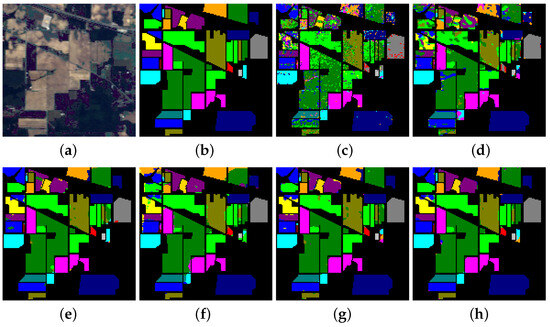
Figure 11.
Classification maps on IP dataset. (a) False-color image. (b) Ground truth. (c) SVM-RBF. (d) M3D-CNN. (e) SSRN. (f) HybridSN. (g) DBMA. (h) Proposed.
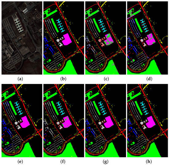
Figure 12.
Classification maps on UP dataset. (a) False-color image. (b) Ground truth. (c) SVM-RBF. (d) M3D-CNN. (e) SSRN. (f) HybridSN. (g) DBMA. (h) Proposed.
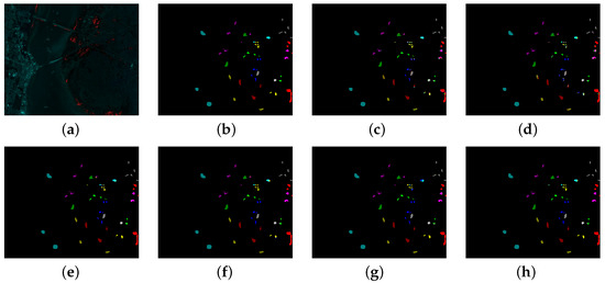
Figure 13.
Classification maps on KSC dataset. (a) False-color image. (b) Ground truth. (c) SVMRBF. (d) M3D-CNN. (e) SSRN. (f) HybridSN. (g) DBMA. (h) Proposed.
4.1. Results on the IP Dataset
As evident in Table 5, for the IP dataset, the proposed method achieved the best classification results with 97.56% for OA, 97.48% for AA, and 97.22% for the Kappa coefficient, the best results for all three metrics. Although our method could not achieve the highest classification accuracy for every category, the accuracy of each category exceeded 91% by performing the classification with our method, which shows that our method is effective at extracting features for different classes. Taking the 15th class Buildings-Grass-Trees-Drives as an example, the accuracies achieved by other methods were 70.29% (SVM-RBF), 88.93% (M3D-CNN), 96.13% (SSRN), 68.87% (HybridSN), and 89.17% (DBMA), while our method obtained an accuracy of 98.47%, with a performance improvement of 2.34–28.18%, and for the class 10 Soybean-notill and class 11 Soybean-mintill, the performance improvement of our method was 2.11–25.52% and 1.46–25.56%, respectively. Compared to other methods, our proposed method improved OA by 0.64–22.82%, AA by 0.41–24.23%, and the Kappa coefficient by 0.73–26.25%.
4.2. Results on the UP Dataset
As the sample size of the UP dataset was large enough, only 0.5% of the training sample was selected in order to verify that our model could achieve excellent results even on small samples. The overall and various classification results for the UP dataset using different methods are shown in Table 6. Both the SSRN and DBMA-based methods have two separate branches for extracting spatial and spectral features, and are more adaptable to the dataset, with OAs of 95.32% and 95.53%, AAs of 94.20% and 94.40%, and Kappa coefficients of 93.81% and 94.07%, respectively. Our proposed approach extends this advantage by invoking superior attention mechanisms and data enhancement methods to improve model performance, with final classification results of 96.85%, 95.25%, and 95.82% for OA, AA, and Kappa coefficients, respectively.
4.3. Results on the KSC Dataset
As observed in Table 7, our proposed method achieved the best results for the classification of the KSC dataset, with the three metrics OA, AA, and Kappa coefficients results being 98.68%, 98.10%, and 98.53%, respectively. The SVM-RBF-based method, due to the loss of spatial information, cannot combine both spatial and spectral information for classification, and it achieves the worst result with an OA of 88.25%. the sample size of the KSC dataset is relatively small, and complex models such as DBMA may overfit the training data, resulting in its OA being inferior to the model constituting the simpler HybridSN, while our proposed model uses multi-scale 2D convolution and multi-layer information fusion strategies to fully extract spatial features in the spatial branch, and a CNN combined with LSTM in the spectral branch to extract and integrate spectral features several times; then, we combined spatial and spectral features to complete the final classification. Compared with other comparison methods, OA improves by 1.21–10.87%.
4.4. Comparison of Running Times of Different Algorithms
The comparative experimental results presented above demonstrate that our proposed algorithm excels in terms of accuracy. To further verify its efficiency, we conducted a comparison of the training and testing times for each algorithm. The time consumption for each algorithm on the IP, UP, and KSC datasets is provided in Table 8, Table 9 and Table 10 (the training time is measured in a total time of 200 epochs). Furthermore, we conducted a comparative analysis of the trainable parameters among CNN-based algorithms to verify the efficiency of our proposed approach. The number of trainable parameters for each algorithm is presented in Table 11.

Table 8.
Training and testing consumption time for different algorithms using 5% training samples on the IP dataset.

Table 9.
Training and testing consumption time for different algorithms using 0.5% training samples on the UP dataset.

Table 10.
Training and testing consumption time for different algorithms using 5% training samples on the KSC dataset.

Table 11.
Trainable parameter for different algorithms using the same hyperparameter.
Since SVM-RBF is a conventional algorithm that does not involve convolutional operations, it took the least time in the comparison experiments for all three datasets. Both SSRN and DBMA have two separate spatial and spectral branches and contain numerous 3D convolutions, which have a large number of parameters and generally take a longer time. Although HybridSN and M3D-CNN are faster than our algorithm, our approach achieved superior accuracy. Moreover, in the comparison of the number of trainable parameters of the model, our proposed model has the fewest parameters among the CNN-based algorithms, which further indicates that the proposed algorithm has higher efficiency. In summary, our algorithm effectively balances accuracy and efficiency.
5. Discussion
In this section, the proposed algorithm is further evaluated by sensitivity analysis. Sensitivity analysis is a method used to assess the response of a model to variations in input parameters. In fields such as air pollution [39,40], sensitivity analysis is crucial for understanding the stability and robustness of systems and identifying key factors. Firstly, for the three datasets, various proportions of training samples are chosen to be infused into the network. The classification results demonstrate that the proposed method consistently performs well, regardless of whether the training samples are large or small. The method’s advantages are particularly pronounced when dealing with relatively small training sample sizes. Secondly, ablation experiments that remove the attention module demonstrate that the attention mechanism contributes to the performance improvement of our method. Thirdly, the number of serial multi-scale convolutional modules is varied for experimental comparison, and it is shown that the best classification OA is obtained by choosing three multi-scale convolutional modules, with neither too many nor too few being optimal.
5.1. Impact of Different Proportions of Training Samples
In this section, we investigate the effect of varying proportions of training samples on the classification results. For the IP and KSC datasets, we choose 1%, 3%, 5%, 8%, and 10% of the labeled samples as training data. For the UP dataset, we select 0.1%, 0.5%, 1%, 5%, and 10% of the labeled samples as training data. Figure 14 illustrates the OA of different models with different proportions of training samples.

Figure 14.
OA of different methods with different proportions of training samples on the datasets of (a) IP, (b) UP, and (c) KSC.
Figure 12 shows that, in cases with a limited number of training samples, our method yields superior classification results and outperforms the other methods. As the training samples increase, the performance of each model improves; when there are enough training samples, the different models achieve near-perfect results with minimal differences, and our method is not weaker than the other methods.
5.2. Impact of the Attention Mechanism
To verify that the attention mechanism has an enhancing effect on classification performance, we conducted the following comparison experiments: removing both spatial and spectral attention modules (no-att), removing the spatial attention module but keeping the spectral attention module (spec-att), removing the spectral attention module but keeping the spatial attention module (spa-att), and keeping both spatial and spectral attention modules (both-att). The results of the comparison experiments are shown in Figure 15.
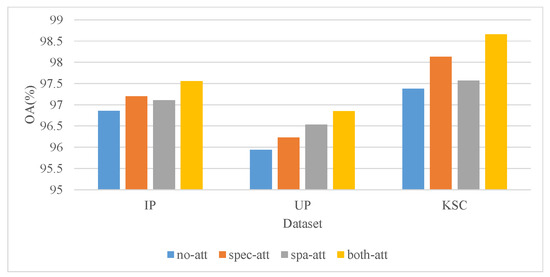
Figure 15.
Impact of the attention mechanism.
The results in the figure illustrate that adding both the spatial attention mechanism module and the spectral attention mechanism module improves the classification accuracy of the HSI. On all three datasets, adding the spectral attention mechanism alone improves OA by 0.29–0.75%, adding the spatial attention mechanism alone improves OA by 0.19–0.59%, and adding both the spatial and spectral attention mechanisms improves OA by 0.7–1.28%, respectively. Overall, the attention mechanism contributes positively to enhanced classification accuracy.
5.3. Impact of the Number of Multi-Scale Convolutional Modules
The results of the experiments shown in Figure 16 confirm that the best results are achieved when the number of multi-scale convolutional feature extraction modules is 3. When the number is too small, spatial features are not fully extracted, while when the number is too large, the model is too complex and prone to overfitting. In the process of increasing the number of multi-scale feature extraction modules from 1 to 5, the OA value exhibits a trend of increasing and then decreasing, and reached a peak when it equals 3.
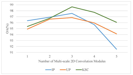
Figure 16.
OA results using different numbers of multi-scale modules.
In short, the results of the sensitivity analysis are as follows: firstly, for different proportions of training samples, our algorithm consistently maintains a superior performance, with the OA increasing and stabilizing with higher proportions of training samples. Secondly, spatial and spectral attention modules enhance the algorithm’s accuracy. Additionally, the number of multi-scale convolution modules needs to be maintained at an appropriate value for the model to achieve optimal performance. Similar to existing algorithms, hyperparameters such as learning rate and the number of hidden units in the LSTM layer need to be kept at suitable values for the model to attain optimal performance.
6. Conclusions
We propose an efficient and lightweight HSI classification framework, SSDBN, which comprises two branches for the extraction of spectral and spatial features, respectively. In the spectral branch, the spectral features are extracted by a combination of a spectral attention mechanism, SSPM, and LSTM modules. In the spatial branch, the spatial features are extracted by the spatial attention mechanism and the multi-scale 2D convolution module, and the output of the multi-level multi-scale module is fused to enhance the classification performance. Comparative experimental results on three popular HSIs demonstrate that our framework outperforms current state-of-the-art algorithms, especially in the case of few samples, and also improves in terms of efficiency due to the abandonment of 3D convolution in favor of 2D convolution, where the parameters of the model are greatly reduced. Therefore, we consider that our proposed algorithm is a qualified HSI classification method. Moreover, the hyperspectral classification work conducted in this paper employs publicly available datasets, and the categories and distribution of ground objects are relatively straightforward compared to real-world scenarios. Consequently, there is a need to supplement the validation of practical application effects using more complex and challenging datasets. Our future work will involve applying the proposed framework to other more complex HSIs and to study more efficient lightweight models for complex HSIs.
Author Contributions
Conceptualization, Y.Z. and J.K.; writing—original draft preparation, Z.C.; writing—review and editing, X.L. and J.K.; project administration, Y.Z. and J.K. All authors have read and agreed to the published version of the manuscript.
Funding
This research was Supported by National Key R&D Program of China (No: 2022YFF0711700), National Cryosphere Desert Data Center (E01Z790201), Research and Development in Artificial Intelligence Data Fusion and Demonstration of Digital Empowerment Applications.
Data Availability Statement
Publicly available datasets were analyzed in this study. This data can be found here https://paperswithcode.com/dataset/indian-pines (accessed on 30 October 2023).
Conflicts of Interest
The authors declare no conflicts of interest.
References
- Mou, L.; Zhu, X.X. Learning to pay attention on spectral domain: A spectral attention module-based convolutional network for hyperspectral image classification. IEEE Trans. Geosci. Remote Sens. 2019, 58, 110–122. [Google Scholar] [CrossRef]
- Tang, Y.; Song, S.; Gui, S.; Chao, W.; Cheng, C.; Fan, F.; Qin, R. Active and Low-Cost Hyperspectral Imaging for the Spectral Analysis of a Low-Light Environment. Sensors 2023, 23, 1437. [Google Scholar] [CrossRef] [PubMed]
- Awad, M.; Jomaa, I.; Arab, F. Improved capability in stone pine forest mapping and management in lebanon using hyperspectral chris-proba data relative to landsat etm+. Photogramm. Eng. Remote 2014, 80, 725–731. [Google Scholar] [CrossRef]
- Marinelli, D.; Bovolo, F.; Bruzzone, L. A novel change detection method for multitemporal hyperspectral images based on binary hyperspectral change vectors. IEEE Trans. Geosci. Remote Sens. 2019, 57, 4913–4928. [Google Scholar] [CrossRef]
- Nolin, A.W.; Dozier, J. A hyperspectral method for remotely sensing the grain size of snow. Remote Sens. Environ. 2000, 74, 207–216. [Google Scholar] [CrossRef]
- Melgani, F.; Bruzzone, L. Classification of hyperspectral remote sensing images with support vector machines. IEEE Trans. Geosci. Remote Sens. 2004, 42, 1778–1790. [Google Scholar] [CrossRef]
- Huang, K.; Li, S.; Kang, X.; Fang, L. Spectral–spatial hyperspectral image classification based on knn. Sens. Imaging 2016, 17, 1–13. [Google Scholar] [CrossRef]
- Li, J.; Bioucas-Dias, J.M.; Plaza, A. Semisupervised hyperspectral image segmentation using multinomial logistic regression with active learning. IEEE Trans. Geosci. Remote Sens. 2010, 48, 4085–4098. [Google Scholar] [CrossRef]
- Huo, L.Z.; Tang, P. Spectral and spatial classification of hyperspectral data using SVMs and gabor textures. In Proceedings of the 2011 IEEE International Geoscience and Remote Sensing Symposium, Vancouver, BC, Canada, 24–29 July 2011; pp. 1708–1711. [Google Scholar]
- Fang, L.; Li, S.; Duan, W.; Ren, J.; Benediktsson, J.A. Classification of hyperspectral images by exploiting spectral–spatial information of superpixel via multiple kernels. IEEE Trans. Geosci. And Remote Sens. 2015, 53, 6663–6674. [Google Scholar] [CrossRef]
- Tarabalka, Y.; Fauvel, M.; Chanussot, J.; Benediktsson, J.A. Svm- and mrf-based method for accurate classification of hyperspectral images. IEEE Geosci. Remote Sens. Lett. 2010, 7, 736–740. [Google Scholar] [CrossRef]
- Redmon, J.; Divvala, S.; Girshick, R.; Farhadi, A. You only look once: Unified, real-time object detection. In Proceedings of the IEEE Conference on Computer Vision and Pattern Recognition, Las Vegas, NV, USA, 27–30 June 2016; pp. 779–788. [Google Scholar]
- Szegedy, C.; Liu, W.; Jia, Y.; Sermanet, P.; Reed, S.; Anguelov, D.; Erhan, D.; Vanhoucke, V.; Rabinovich, A. Going deeper with convolutions. In Proceedings of the IEEE Conference on Computer Vision and Pattern Recognition, Boston, MA, USA, 7–12 June 2015; pp. 1–9. [Google Scholar]
- Bordes, A.; Glorot, X.; Weston, J.; Bengio, Y. Joint learning of words and meaning representations for open-text semantic parsing. In Artificial Intelligence and Statistics; PMLR: La Palma, Canary Islands, Spain, 2012; pp. 127–135. [Google Scholar]
- Chen, Y.; Lin, Z.; Zhao, X.; Wang, G.; Gu, Y. Deep learning-based classification of hyperspectral data. IEEE J. Sel. Top. Appl. Earth Obs. Remote Sens. 2014, 7, 2094–2107. [Google Scholar] [CrossRef]
- Li, T.; Zhang, J.; Zhang, Y. Classification of hyperspectral image based on deep belief networks. In Proceedings of the 2014 IEEE International Conference on Image Processing (ICIP), Paris, France, 27–30 October 2014; pp. 5132–5136. [Google Scholar]
- Hu, W.; Huang, Y.; Wei, L.; Zhang, F.; Li, H. Deep convolutional neural networks for hyperspectral image classification. J. Sens. 2015, 2015, 258619. [Google Scholar] [CrossRef]
- Makantasis, K.; Karantzalos, K.; Doulamis, A.; Doulamis, N. Deep supervised learning for hyperspectral data classification through convolutional neural networks. In Proceedings of the 2015 IEEE International Geoscience and Remote Sensing Symposium (IGARSS), Milan, Italy, 26–31 July 2015; pp. 4959–4962. [Google Scholar]
- Chen, Y.; Jiang, H.; Li, C.; Jia, X.; Ghamisi, P. Deep feature extraction and classification of hyperspectral images based on convolutional neural networks. IEEE Trans. Geosci. Remote Sens. 2016, 54, 6232–6251. [Google Scholar] [CrossRef]
- Roy, S.K.; Krishna, G.; Dubey, S.R.; Chaudhuri, B.B. Hybridsn: Exploring 3-d–2-d cnn feature hierarchy for hyperspectral image classification. IEEE Geosci. Remote Sens. Lett. 2019, 17, 277–281. [Google Scholar] [CrossRef]
- He, M.; Li, B.; Chen, H. Multi-scale 3d deep convolutional neural network for hyperspectral image classification. In Proceedings of the 2017 IEEE International Conference on Image Processing (ICIP), Beijing, China, 17–20 September 2017; pp. 3904–3908. [Google Scholar]
- Zhong, Z.; Li, J.; Luo, Z.; Chapman, M. Spectral–spatial residual network for hyperspectral image classification: A 3-d deep learning framework. IEEE Trans. Geosci. Remote Sens. 2017, 56, 847–858. [Google Scholar] [CrossRef]
- Mei, X.; Pan, E.; Ma, Y.; Dai, X.; Huang, J.; Fan, F.; Du, Q.; Zheng, H.; Ma, J. spectral–spatial Attention Networks for Hyperspectral Image Classification. Remote Sens. 2019, 11, 963. [Google Scholar] [CrossRef]
- Li, Z.; Zhao, X.; Xu, Y.; Li, W.; Zhai, L.; Fang, Z.; Shi, X. Hyperspectral image classification with multiattention fusion network. IEEE Geosci. Remote Sens. Lett. 2021, 19, 5503305. [Google Scholar] [CrossRef]
- Ma, W.; Yang, Q.; Wu, Y.; Zhao, W.; Zhang, X. Double-branch multi-attention mechanism network for hyperspectral image classification. Remote Sens. 2019, 11, 1307. [Google Scholar] [CrossRef]
- Xu, Y.; Du, B.; Zhang, F.; Zhang, L. Hyperspectral image classification via a random patches network. ISPRS J. Photogramm. Remote 2018, 142, 344–357. [Google Scholar] [CrossRef]
- Sherstinsky, A. Fundamentals of recurrent neural network (rnn) and long short-term memory (lstm) network. Phys. Nonlinear Phenom. 2020, 404, 132306. [Google Scholar] [CrossRef]
- Zuo, Z.; Shuai, B.; Wang, G.; Liu, X.; Wang, X.; Wang, B.; Chen, Y. Learning contextual dependence with convolutional hierarchical recurrent neural networks. IEEE Trans. Image Process. 2016, 25, 2983–2996. [Google Scholar] [CrossRef] [PubMed]
- Hang, R.; Liu, Q.; Hong, D.; Ghamisi, P. Cascaded recurrent neural networks for hyperspectral image classification. IEEE Trans. Geosci. Remote Sens. 2019, 57, 5384–5394. [Google Scholar] [CrossRef]
- Hochreiter, S.; Schmidhuber, J. Long short-term memory. Neural Comput. 1997, 9, 1735–1780. [Google Scholar] [CrossRef] [PubMed]
- Gers, F.A.; Schmidhuber, E. Lstm recurrent networks learn simple context-free and context-sensitive languages. IEEE Trans. Neural Netw. 2001, 12, 1333–1340. [Google Scholar] [CrossRef] [PubMed]
- Bukhari, A.H.; Raja, M.A.Z.; Sulaiman, M.; Islam, S.; Shoaib, M.; Kumam, P. Fractional neuro-sequential arfima-lstm for financial market forecasting. IEEE Access 2020, 8, 71326–71338. [Google Scholar] [CrossRef]
- He, N.; Paoletti, M.E.; Haut, J.M.; Fang, L.; Li, S.; Plaza, A.; Plaza, J. Feature extraction with multi-scale covariance maps for hyperspectral image classification. IEEE Trans. Geosci. Remote Sens. 2018, 57, 755–769. [Google Scholar] [CrossRef]
- Gong, H.; Li, Q.; Li, C.; Dai, H.; He, Z.; Wang, W.; Li, H.; Han, F.; Tuniyazi, A.; Mu, T. multi-scale information fusion for hyperspectral image classification based on hybrid 2d-3d cnn. Remote Sens. 2021, 13, 2268. [Google Scholar] [CrossRef]
- Gong, Z.; Zhong, P.; Yu, Y.; Hu, W.; Li, S. A cnn with multi-scale convolution and diversified metric for hyperspectral image classification. IEEE Trans. Geosci. Remote Sens. 2019, 57, 3599–3618. [Google Scholar] [CrossRef]
- Wang, Q.; Wu, B.; Zhu, P.; Li, P.; Zuo, W.; Hu, Q. ECA-net: Efficient channel attention for deep convolutional neural networks, 2020 IEEE. In Proceedings of the CVF Conference on Computer Vision and Pattern Recognition (CVPR), Seattle, WA, USA, 13–19 June 2020; pp. 11531–11539. [Google Scholar]
- Zhang, X.; Shang, S.; Tang, X.; Feng, J.; Jiao, L. Spectral partitioning residual network with spatial attention mechanism for hyperspectral image classification. IEEE Trans. Geosci. Remote Sens. 2022, 60, 5507714. [Google Scholar] [CrossRef]
- Woo, S.; Park, J.; Lee, J.-Y.; Kweon, I.S. CBAM: Convolutional block attention module. In Proceedings of the European Conference on Computer Vision (ECCV), Munich, Germany, 8–14 September 2018; pp. 3–19. [Google Scholar]
- Todorov, V.; Dimov, I. Unveiling the Power of Stochastic Methods: Advancements in Air Pollution Sensitivity Analysis of the Digital Twin. Atmosphere 2023, 14, 1078. [Google Scholar] [CrossRef]
- Todorov, V.; Dimov, I.; Ostromsky, T.; Dimov, I.; Zlatev, Z.; Georgieva, R.; Poryazov, S. Optimized Quasi-Monte Carlo Methods Based on Van der Corput Sequence for Sensitivity Analysis in Air Pollution Modelling. In Recent Advances in Computational Optimization: Results of the Workshop on Computational Optimization WCO 2020; Springer: Cham, Switzerland, 2022; pp. 389–405. [Google Scholar]
Disclaimer/Publisher’s Note: The statements, opinions and data contained in all publications are solely those of the individual author(s) and contributor(s) and not of MDPI and/or the editor(s). MDPI and/or the editor(s) disclaim responsibility for any injury to people or property resulting from any ideas, methods, instructions or products referred to in the content. |
© 2024 by the authors. Licensee MDPI, Basel, Switzerland. This article is an open access article distributed under the terms and conditions of the Creative Commons Attribution (CC BY) license (https://creativecommons.org/licenses/by/4.0/).