Abstract
Hyperspectral images (HSIs) are widely used to identify and characterize objects in scenes of interest, but they are associated with high acquisition costs and low spatial resolutions. With the development of deep learning, HSI reconstruction from low-cost and high-spatial-resolution RGB images has attracted widespread attention. It is an inexpensive way to obtain HSIs via the spectral reconstruction (SR) of RGB data. However, due to a lack of consideration of outdoor solar illumination variation in existing reconstruction methods, the accuracy of outdoor SR remains limited. In this paper, we present an attention neural network based on an adaptive weighted attention network (AWAN), which considers outdoor solar illumination variation by prior illumination information being introduced into the network through a basic 2D block. To verify our network, we conduct experiments on our Variational Illumination Hyperspectral (VIHS) dataset, which is composed of natural HSIs and corresponding RGB and illumination data. The raw HSIs are taken on a portable HS camera, and RGB images are resampled directly from the corresponding HSIs, which are not affected by illumination under CIE-1964 Standard Illuminant. Illumination data are acquired with an outdoor illumination measuring device (IMD). Compared to other methods and the reconstructed results not considering solar illumination variation, our reconstruction results have higher accuracy and perform well in similarity evaluations and classifications using supervised and unsupervised methods.
1. Introduction
Compared with RGB images, HSIs are characterized by the combination of spatial and spectral information. Due to numerous spectral bands, HSIs can capture the spectral distribution, which is helpful to describe the detailed spectral characteristics of the scene. The abundant spectral information of HSIs is beneficial to numerous applications such as those for object detection [1,2,3], classification [4,5,6], segmentation [7], face recognition [8] and other aspects.
Although hyperspectral devices have many obvious advantages, the following factors limit their further application: (1) due to the complexity of their optical systems, most hyperspectral devices are too heavy to be mounted on portable platforms, such as drones and hand-held cameras [9]; (2) hyperspectral devices are expensive and not easily affordable [10]; and (3) the long-term acquisition of HSIs results in spatial and spectral degradation, which is unsuitable for rapid acquisition or scenes with moving objects [11].
Compared to hyperspectral devices, RGB cameras have the advantages of smaller sizes, lighter weights, shorter imaging times, higher signal-to-noise ratios, and minor geometric deformations [12]. The reconstruction of HSIs using RGB images can overcome many of the limitations of existing hyperspectral instruments and combine the advantages of HSIs and RGB images. In this way, high-precision and high-quality HSIs can be obtained using low-cost equipment, and the spectral resolutions of existing RGB cameras can be improved [11].
The essence of reconstructing HSIs from RGB images is to learn the mapping relationship of the spectral dimension between corresponding pixels. This is a sick problem [13]. Prior to the rise of deep learning, there was a lot of research on learning the mapping of RGB images to the the corresponding HSIs. Some early methods for RGB spectral recovery images relied on linear models that adopted statistical analysis strategies, which assumed that 3–10 basis functions can usually represent HSIs. Then, most methods were based on PCA [14,15] or the matrix R approach [16]. However, sparse coding approaches outperformed them quickly [17,18]. In recent years, with the development of computer hardware and the abundance of datasets, deep learning methods have caused wide concern. Deep learning has shown outstanding ability in image generation [19,20,21], and Goodfellow et al. [19] introduced generative adversarial networks (GANs), a framework that significantly advanced image generation. GANs employ adversarial training between a generator and a discriminator, leading to the synthesis of realistic images by mapping random noise to the target data distribution. Isola et al. [20] make a significant contribution to image generation through conditional adversarial networks. It introduces an effective approach for image-to-image translation, enabling the synthesis of realistic and high-quality images in various visual domains. Dong et al. [21] propose an accelerated super-resolution convolutional neural network (SRCNN). Their work focuses on enhancing the efficiency of super-resolution tasks, providing a valuable advancement in generating high-quality and detailed images. A series of CNN-based SR models is also presented to learn a mapping function from a single RGB image to its corresponding HSI [22,23,24,25,26,27]. Xiong et al. [24] present an innovative contribution with an HSCNN, a convolutional neural network (CNN) designed for the recovery of hyperspectral images from spectral projections. This work addresses the challenge of reconstructing high-quality hyperspectral imagery from limited spectral information, offering advancements in the field of image recovery. Kaya et al. [22] focus on spectral estimation from a single RGB image in real-world scenarios, addressing the challenges posed by diverse environmental conditions. Arad et al. [23] emphasize spectral reconstruction from RGB images and foster benchmarking in the field. Fu et al. [25] introduce a novel approach for coded hyperspectral image reconstruction, leveraging deep external and internal learning methods. Their work enhances the efficiency of spectral recovery processes. Shi et al. [26] present an HSCNN+, an advanced CNN-based method for hyperspectral recovery from RGB images. Their contribution lies in the development of an effective model for reconstructing hyperspectral information, demonstrating superior performance in comparison to existing methods. Li et al. [27] propose a progressive spatial–spectral joint network for hyperspectral image reconstruction, introducing a novel approach that integrates spatial and spectral information progressively.
Illumination is an important source of error in SR. It mainly causes the variation in the intensity and angle of incident light. Nguyen et al. show the reconstruction result without considering the illumination is not robust, so the white balance method is used to improve the accuracy of the result and make the result more robust [28]. This variation will affect the radiance of objects. Fu et al. prove that illumination has an impact on the accuracy of reconstructed images. They improve the model to reconstruct high-precision hyperspectral images under different illumination conditions [13]. In order to improve the accuracy of reconstruction, some methods have considered the effect of illumination on SR. Chi et al. develop an approach by leveraging optimized wide-band filtered illumination [29]. Nguyen et al. present a strategy to model the mapping relationship between RGB values which are acquired by camera and scene spectral by using training images [28].
However, due to a lack of consideration of outdoor solar illumination variation in existing reconstruction methods, the accuracy of outdoor SR remains limited, especially for long-term HS imaging. To address this weakness, we develop an attention network based on prior inter-frame illumination variation information. Our network is based on AWAN [10], which performs well in SR. AWAN consists of a dual residual attention block (DRAB) and a patch-level second-order non-local (PSNL) module. It can not only allow abundant low-frequency information to be bypassed to enhance feature correlation learning but also capture long-range spatial contextual information. The outdoor solar illumination is fed into the network via a basic 2D block. As a weighted attention mechanism, the weights can guide the network to generate HSIs in which the solar illumination variation is corrected. Finally, to make full use of the low-frequency features of RGB images, we sum the output of AWAN and RGB features after a layer of convolution.
The main contributions of this paper are summarized as follows.
(1) The consideration of the impact of solar illumination variation on UAV hyperspectral imaging. To minimize the influence of illumination variation on SR, we conduct relative illumination correction on the push-broom line of each hyperspectral image to generate HSI and RGB data, which are not affected by solar illumination variation. This method of reconstruction closely represents the outdoor situations of imaging.
(2) The presentation of an attention network framework based on prior inter-frame outdoor solar illumination variation information. The backbone of the proposed network is based on an AWAN. The illumination information is introduced into the network as prior information via the basic 2D block to reconstruct HSIs from RGB images more accurately.
(3) The collection of hyperspectral dataset with a spectral range of 400–1000 nm using an unmanned aerial vehicle (UAV). The dataset contains 120 images and labels of illumination information. The illumination information precisely corresponds to GPS time. Compared to all existing datasets, our dataset is for UAV reconstruction that considers outdoor solar illumination variation. It can provide support for research into outdoor spectral imaging, processing, and analysis in the future.
2. Related Works
In order to intuitively present the changes in characteristics of the outdoor observed object or region, it is necessary to consider the effects of solar illumination and atmospheric factors during imaging to improve the accuracy of SR.
2.1. Influence of Outdoor Illumination Variation
Scholars consider the influence of illumination, and the experimental results show that illumination is an important factor in spectral reconstruction. A stable light source is generally used for illumination in laboratories, so there are no influences from atmospheric variation. The intensity and incident angle of outdoor illumination change over time, which causes variation in the radiance received by sensors and multiple scattering between objects [30,31,32]. Ximena et al. [33] studied the influence of incident illumination on spectral data acquisition at different times and dates. J. Pablo et al. [34] evaluated the effects of push-broom hyperspectral cameras on imaging under various outdoor illumination conditions.
Some methods have considered the effect of illumination on spectral reconstruction. Nguyen et al. [28] present a radial basis function network that uses white balancing to reconstruct spectral reflectance images from single RGB images. This white-balance step helps to make the approach robust to input images captured under illumination conditions that are not represented in the training data. To obtain multispectral reflectance information, Park et al. propose a multiplexed illumination technique to recover the continuous spectral information for each scene point using a linear model for spectral reflectance [35]. All above methods try to remove or reduce the illumination effect and conduct SR. However, variation in outdoor solar illumination is ignored.
2.2. Influence of Time Measurements Mismatch
Jong-Min et al. [36] composed a dual ASD FieldSpec® 3 system with two mutually calibrated ASD spectrometers. This system simultaneously used two radiometers for mutual calibration and wireless synchronization and also simultaneously collected the reference spectra of standard boards and the spectra of sample targets. The main purpose of the system is to eliminate the errors caused by the variation in illumination conditions when the measurement time is not strictly synchronized. Burkart et al. [37] use two marine optical spectrometers: one mounted on a multirotor UAV to measure the spectra of ground objects and the other to measure standard plates on the ground. This method calculates reflection coefficients through the continuous measurement of target and Lambert reference panels. All of the above scholars take into account the influence of outdoor solar illumination variation on HS measurement calculations and aim to reduce the errors caused by solar illumination variation and target measurement time asynchronicity. It only takes a short time to collect RGB images of scenes. However, HSIs are acquired by spatial push-broom or band-wise models; this way takes a long time. Due to the longer acquisition times, outdoor solar illumination variation becomes a source of errors in SR. In real imaging scenes, solar illumination variation cannot be ignored in spectral reconstruction.
To conduct high-precision SR, it is necessary to consider changes in the environment during the acquisition period. If these variations are not considered, the reconstructed results can only represent the virtual HS information at the moments when the RGB images are taken rather than being closely representative of the real results collected by HS instruments under real conditions. During the process of SR, differences in acquisition times are mainly caused by the frame frequency limits of spectroscopic systems and detectors. The imaging times of HS cameras are usually longer than those of RGB cameras. Generally, the instruments used for spectral acquisition extend acquisition times to improve the signal-to-noise ratio (SNR). It is necessary to consider the real imaging environment during HSI reconstruction from RGB images. The purpose of SR is to obtain hyperspectral curves via high-cost acquisition methods and analyze the composition properties of substances, which is very important to ensure the accuracy of SR [13,18,38,39,40,41].
CNN-based reconstruction algorithms do not depend too much on specific instrument acquisition systems. Nie et al. [42] advocate a network which based on U-net to learn the filter response functions in the infinite space of nonnegative and smooth curves. Li et al. [10] develop a deep adaptive weighted attention network for SR. This model is proposed to adaptively recalibrate channel-wise feature responses by exploiting adaptive weighted feature statistics. Fu et al. [13] present an efficient network that can jointly select the optimal camera spectral response (CSR) and learn mapping functions to recover HSIs from single RGB images captured with an algorithmically selected camera. Xiong et al. [24] propose a general deep-learning network framework for spectral reconstruction and achieve good results for coded aperture snapshot spectral imaging (CASSI). Zhang et al. [43] present a pixel-aware deep function-mixture network for super-resolution spectral information that can flexibly handle pixels from different categories or spatial positions within HSIs. Han et al. [44] obtained super-resolution spectral information using a spectral reconstruction CNN, which can use the available RGB images to predict the high-frequency content of fine spectral wavelengths in narrowband intervals. Yan et al. [39] introduce a novel framework based on U-Net (C2H-Net), which can reconstruct HSIs using prior information about the classification and location of objects, especially for targets with similar RGB features.
3. Data and Method
3.1. Data
We evaluate the proposed network on our VIHS dataset. The VIHS dataset comprises natural HSIs and the corresponding illumination information. The dataset includes 16 scenes, 100 images for training, 10 images for testing, and 10 images for validation. Several test images are presented in Figure 1.

Figure 1.
Sample images from the our VIHS dataset.
3.1.1. Illumination Data
The outdoor illumination measuring device (IMD) which is used in this study consists of an ASD, optical fibers, and a cosine corrector (Figure 2). In addition, the solar irradiance at each moment is recorded using GPS time, which is convenient for time matching each frame of data collected by the hyperspectral camera. The cosine corrector can increase the accuracy of solar downward radiation measurement [45]. The spectral resolution obtained by the ASD is 1 nm. To ensure that the solar illumination can be measured by the ASD and the HSIs have the same spectral resolution, the spectral resampling method is adopted to preprocess the illumination data. Figure 3 shows the outdoor solar illumination variation over time.
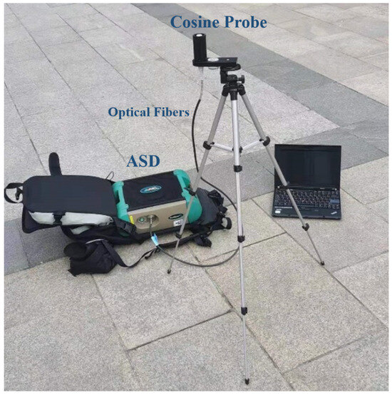
Figure 2.
The outdoor variant illumination measuring device (IMD).
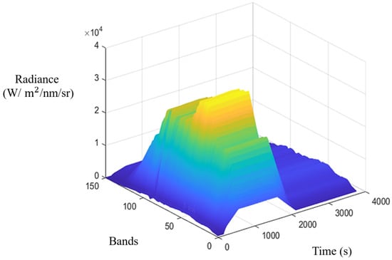
Figure 3.
The example of outdoor solar illumination variation over time.
3.1.2. HSI Data
The raw HSIs in the VIHS dataset are taken on a portable HS camera (Corning® microHSI™ 410 SHARK [46]) with a spatial resolution of 1364 pixels, a spectral resolution of 4 nm, and 150 spectral bands from 400 to 1000 nm. When we collect the images, the camera is mounted on a UAV. The flight height is 100 m. The solar irradiance observation equipment is placed in a wide-view area. We use the calibration coefficient of the instrument to convert the image digital number (DN) values into radiance and obtain the hyperspectral radiance images. The GPS time is recorded when each frame is acquired by the camera, which can be used to match the time recorded by the IMD.
The processing of each scene of hyperspectral image consists of three parts. Firstly, the first frame of the hyperspectral radiance image is taken as the standard frame, and the IMD time corresponding to this frame is taken as the standard time. The illumination value of standard time is used as the reference, and the illumination correction coefficients are obtained by dividing the illumination value of IMD corresponding to other frame time. Secondly, we take the standard frame as the benchmark, the remaining frames of the hyperspectral radiance image are corrected by the coefficients to obtain the hyperspectral radiance image which is not affected by illumination. The purpose of this step is to obtain RGB image that is not affected by solar illumination variation. All kinds of images have been cropped to a size of 512 × 482 to be consistent with the existing reconstructed dataset.
3.1.3. RGB Data
RGB images of the VIHS dataset are resampled directly from the hyperspectral radiance image that is not affected by illumination under CIE-1964 Standard Illuminant. Since the hyperspectral radiance image not affected by illumination is corrected with illumination, the generated RGB is actually illumination independent. This is in line with the characteristics of general RGB cameras, i.e., no push-broom, less time, and near-instantaneous imaging.
3.2. Method
In this section, we first formulate the problem. Then, the SR is presented. Finally, we provide the learning details.
3.2.1. Formulation
When acquiring an image using a RGB or monochromatic camera, the radiance Y at the location of RGB is:
where denotes the CSR function. represents that spectral radiance of HSI at the location . However, when HS data are collected outdoors, changes with push-broom time. Then, we calculate the illumination correction coefficients as below:
denotes the illumination value of imaging moment t. represents the illumination value of standard time, which is treated as the reference. In this process, the illumination I needs to be resampled to remain consistent with the spectral resolution of HSI.
We can represent the radiance with the illumination correction as follows:
t is the imaging time with the frame of each HSI. In reality, the discrete representation is the formula below:
where represents the wavelength at the n-th spectral band, usually . According to the above formula, illumination is an important factor for SR.
3.2.2. Architecture of Network
The entire network structure is shown in Figure 4. The network consists of two convolutions, a basic 2D block (as shown in Figure 5), and a backbone AWAN (as shown in Figure 6), which was proposed by Li et al. [10] and performs well for spectral reconstruction.
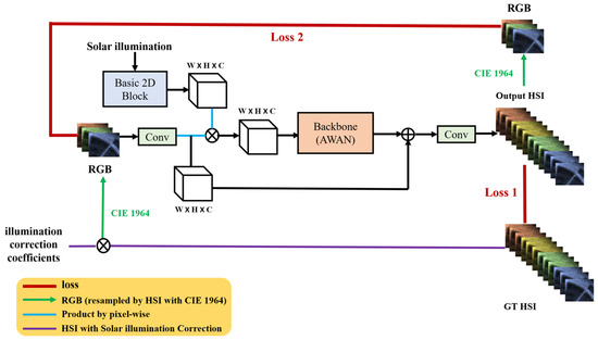
Figure 4.
The whole network architecture for SR.

Figure 5.
The architecture of basic 2D block.

Figure 6.
The architecture of AWAN.
We add the illumination data to our network via the basic 2D block, as shown in Figure 5. The basic 2D block consists of two convolutions and a ReLU. The convolutions are used to extract illumination features and the ReLU is used for the nonlinear activation function.
The AWAN consists of 12 dual residual attention blocks (DRABs) (as shown in Figure 7) and a PSNL module (as shown in Figure 8). Each DRAB consists of a residual module, convolutional operations with different kernel sizes, and adaptive weighted channel attention (AWCA), as shown in Figure 9. Long and short skip connections are contained in the block. This module can make full use of the abundant low-frequency information in the input images and enhance feature correlation learning. The AWCA module is adopted for stronger feature correlation.

Figure 7.
The architecture of DRAB.

Figure 8.
The architecture of PSNL.

Figure 9.
The architecture of AWCA.
Given a set of intermediate feature maps , the size of the feature map is . The number of feature maps is C. is reshaped to , and we reshape to . Then, softmax is adopted to normalize , and we multiply with , and adaptive weighted pooling can be represented as below:
where is the channel-wise descriptors. In order to exploit the aggregated information of adaptive weighted pooling, AWAC employs sigmoid and two convolutional layers. The final channel map is computed as:
where and denote two convolutional layers. and represent sigmoid and ReLU, respectively. Then, we assign the channel feature map to rescale the input . The output feature map of the AWAC module is obtained as follows:
The AWCA module can adjust channel-wise features to adaptively recalibrate, thereby enhancing the network’s representation capabilities.
The PSNL is used to model distant region relationships simultaneously. The inputs for the PSNL are divided into four sub-feature maps (, where a = 1, 2, 3, 4). When the sub-feature map is fed into two convolutions with 1 × 1 kernel size, we obtain the new sub-feature maps and , which we can then reshape and transpose. The spatial attention map can be represented as , where and denote the identity matrix and the all-ones matrix, respectively. Then, we compute as below:
Then, the is fed to a convolution . We obtain the final output .
The purple line in Figure 4 shows that the illumination correction is performed before resampling HSIs into RGB images, which aims to greatly restore the situation of RGB imaging. To simplify the network, this operation is finished in the preprocessing stage. The green line in the figure represents resampling HSIs into RGB images using the CIE-1964 standard illuminant.
3.2.3. Loss Function
Generally, we adopt the mean relative absolute error (MRAE) as a loss function instead of the mean square error (MSE). As it is affected by illumination and atmospheric factors, the radiance of ground objects in different bands varies greatly and MSE has limitations for this kind of problem. Our HSI reconstruction network can be optimized by minimizing the MRAE between a reconstructed HSI and the corresponding ground truth (GT) image . The formula for MRAE is as below:
i, j represent the row and column of feature maps, respectively, and n denotes the channel.
Li et al. [10] suggest the CSR prior is important for more accurate reconstruction. The CSR function can represent the discrepancies of RGB images resampled from GT HSI and reconstruct HSI more finely; the CSR function is shown as below:
Then, we combine these two loss functions.
where denotes CSR function, which is the CIE-1964 color-matching function. is hyper-parameter. The value of is set to 10 empirically.
4. Experiment
4.1. Experimental Setup
Our approach is implemented in the PyTorch framework with a NVIDIA RTX 3080 GPU. The backbone of our network adopts a pre-trained model which is trained on the NTIRE2020 dataset [23]. The whole model is also trained on our training set. In the training phase, we set the mini-batch size to 16 and the parameters of the Adam optimization algorithm as , , and to minimize our loss. During the training, we crop sample pairs of RGB images and HSIs to . The learning rate is initialized as and the polynomial function is set to decay by the power of 1.5. We stop the network training after 100 epochs. The training and validation loss curves are shown in Figure 10. The RMSE is used to evaluate the validation results more intuitively.
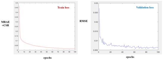
Figure 10.
The training and validation loss curves.
4.2. Evaluation Metrics
We adopt qualitative and quantitative evaluation metrics to compare the differences between our reconstructed results and the GT results.
The overall accuracy is evaluated by MRAE and RMSE.
In order to analyze the similarity of spectral and spatial features between the reconstructed result and GT, Pearson correlation coefficient (CC) [47], and peak signal-to-noise ratio (PSNR), and the absolute error (AE) between the GT and reconstructed result are used to calculate pixel-wise [48].
4.3. Experimental Results
Figure 11 shows the false color reconstruction results of HSCNN+, HRNet [49], our proposed method (with/without considering illumination variation), and the GT results, which are used to demonstrate the reconstruction effect and visual evaluation of image quality. Our method without considering illumination variation uses the AWAN architecture. In terms of visual effects, our reconstructed images are similar to the GT results in color, texture, and shape.
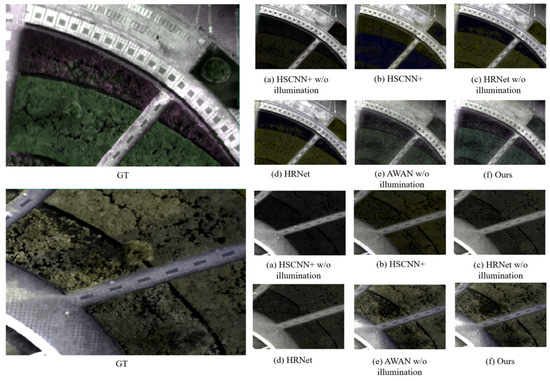
Figure 11.
False color composite of two reconstructed images and GT examples of our dataset. (a) Reconstructed HSI with considering solar illumination variation; (b) reconstructed HSI w/o considering solar illumination variation; (c) GT.
We present an example to analyze the spatial characteristics of the errors. In Figure 12, rows 3, 4, and 5 show the reconstructed images with/without solar illumination variation and the GT images, respectively. It can be seen from the figure that the reconstructed and GT images of the four selected bands are similar. The corresponding AE maps are shown in rows 1 and 2 in Figure 12 and the color distributions of the error graphs present that the reconstruction errors are very small in all four bands. As the value bars of the AE maps show, the reconstructed images without consideration of solar illumination variation have wider error value ranges than the reconstructed results with solar illumination variation.
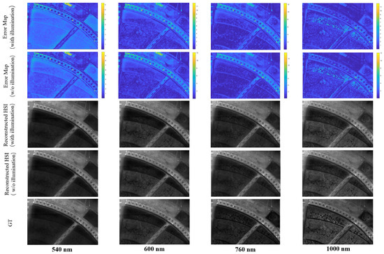
Figure 12.
Spatial characteristics of errors. From top to bottom: AE with considering illumination variation, AE w/o considering solar illumination variation, reconstructed HSI with considering solar illumination variation, reconstructed HSI w/o considering solar illumination variation, and GT. From left to right: 540 nm, 600 nm, 760 nm, and 1000 nm. The scale at the top represents the value of AE.
Table 1 shows the average accuracy of reconstructed HSIs on the test set with different methods with and without considering illumination variation. The MRAE and RMSE values for our reconstructed results with solar illumination variation on our dataset are 0.2298 and 0.0399; the values are lower than those for the reconstructed results without considering solar illumination variation. The RMSE value is reduced by a certain order of magnitude and the MARE is reduced by 0.1493. This demonstrates that the absolute accuracy of the reconstructed HSIs is high and have a better spectral reconstruction effect. The errors between our reconstructed results considering solar illumination variation and the GT results are smaller than those between the reconstructed results without considering solar illumination variation and the GT results. The PSNR and CC values of our reconstructed results considering solar illumination variation are 77.7594 and 0.9496. They are higher than the results without considering solar illumination variation. It can indicate that our reconstructed results considering solar illumination variation are more similar to the GT results. Outdoor solar illumination variation is random and irregular. When the conditions are close to real imaging environments and with real imaging instruments, this random phenomenon affects network learning when the solar illumination variation factor is not considered during reconstruction. Our reconstruction results are better than the listed method (considering or not considering illumination variation) in both qualitative and quantitative aspects. Therefore, we collect illumination data and input them into the model as constraints in the form of vectors, so our model can more accurately map RGB images to HSIs.

Table 1.
Quantitative evelation of reconstruction results.
Figure 13 shows the spectral curves of roads, shrubs, and grass. On the whole, the curves of the reconstructed HSIs considering illumination variation are more similar to the GT curves than those of the reconstructed HSIs without considering illumination variation for all selected objects from our dataset. By comparing the images of the road in Figure 13b, it can be seen that the curve of the reconstructed image considering illumination variation is closer to that of the GT image and that with the increase in wavelength, the accuracy tends to improve gradually. The overall trend is roughly similar for the reconstructed images without considering illumination variation, but the accuracy is significantly lower when the band is nearer to the blue and near-infrared bands. The atmospheric scattering of sunlight in the blue band is relatively strong. With outdoor illumination variation, the intensity of the scattering and the energy received by ground objects in this band also change. These variations affect the reconstruction accuracy. In our study, when illumination variation is considered, the accuracy curves tend to be stable with the increase in wavelength. This is consistent with the law that atmospheric scattering decreases with increasing wavelength. Figure 13c,d compare the spectral reconstruction results for different plant types. By comparing the reconstructed results in Figure 13c, it can be seen that the reconstructed results for grass in different scenes are more stable when illumination is considered. The results without considering illumination variation are quite different from the GT results in terms of both overall trend and value. The reconstructed results obtained with our model are more stable. In Figure 13d, the reconstructed results of shrubs in different scenes are compared. The error curves of the top and bottom images are consistent, and the accuracy is better than when illumination is not considered. By comparing Figure 13c,d, it can be concluded that the reconstruction accuracy and stability within the plant category are greatly improved by considering illumination variation. The above analysis shows that the proposed network has better spatial and spectral adaptability.
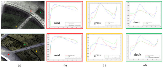
Figure 13.
The spectral curves of GT and reconstructed images from our dataset, both considering and w/o considering solar illumination variation: (a) the original HSI (the red star shows the location of the road, the yellow star shows the location of the grass, and the green star shows the location of the shrub); (b) the spectral curves of the road; (c) the spectral curves of the grass; (d) the spectral curves of the shrub.
4.4. Image Classification and Accuracy Comparison
To further validate the quality of our HSI reconstruction, classification experiments are conducted on the reconstructed HSIs and the GT images. Qualitative visual effects and quantitative accuracy evaluation metrics are employed to evaluate the spatial and spectral consistency between the reconstructed images and the GT images.
We use the support vector machine (SVM) supervised classifier and the iterative self-organizing data analysis algorithm (IsoData) unsupervised classifier. The SVM and IsoData are conducted in ENVI 5.3. We extract the specific targets, namely road, grass, and shrub, from the GT samples using the SVM classifier. The detailed parameters of the IsoData ENVI settings are shown in Table 2.

Table 2.
The detailed parameters of IsoData ENVI setting.
We adopt the classification GT results as the reference for the unsupervised IsoData classification method and quantitatively calculate the similarity index (SI) between the classification results of our reconstructed HSIs and those of the GT images:
where Q is the number of pixels in the same classified category of reconstructed HSI and GT, K denotes the total number of pixels in the whole image. For the SVM classifier, we not only calculate SI between the classification results of our reconstructed HSI and GT but also evaluate the classification accuracy with overall accuracy (OA) and the kappa coefficient (Kappa).
The classification results of unsupervised method IsoData are shown in Figure 14. The classification results of most objects are similar with the classification results of GT from the visual effect.
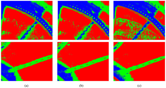
Figure 14.
Unsupervised classification IsoData results based on our dataset. (a) Classification of reconstruction with considering solar illumination variation; (b) classification of reconstruction w/o considering solar illumination variation; (c) GT classification.
Figure 15 shows the classification results from the SVM. Due to the indistinguishability of shrubs and grass, there are some errors in the unsupervised classification.
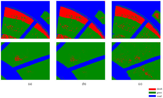
Figure 15.
SVM classification results based on our dataset. (a) Classification of reconstruction with considering solar illumination variation; (b) classification of reconstruction w/o considering solar illumination variation; (c) GT classification.
Then, we calculate the average SI between the classification results of the reconstructed HSIs and those of the GT images, as shown in Figure 14. The IsoData classification SI values for the reconstructed HSIs considering and without considering illumination variation are 81.80% and 80.26%, respectively. The average SI value of the reconstructed HSIs considering illumination variation using the IsoData classifier is 1.54% higher than that of the reconstructed HSIs without considering illumination variation.
Table 3 shows the average classification accuracy and the SI, OA, and Kappa values from the SVM classifier. Using the SVM classification method, the SI value of the reconstructed HSIs considering and without considering illumination variation are 87.76% and 86.12%, respectively. The similarity, OA, and Kappa values of the reconstructed HSIs considering illumination variation are higher than those of the reconstructed HSIs without considering illumination variation. On the whole, the results demonstrate that reconstructed HSIs can be used for classification and that the reconstructed classification results considering illumination variation are better than those without considering illumination variation.

Table 3.
Quantitative classification results of SVM (GT, reconstructed HSI with IV (illumination variation), reconstructed HSI without IV).
In addition, in our method, a softmax layer is used to normalize the feature. To make use of the aggregated information by adaptive weighted pooling, we adopt a simple gating mechanism with sigmoid function. ReLU is essentially a function that takes the maximum value. If the input is negative, it will output 0, and the neuron will not be activated. In future research, we will adopt the adaptive activation functions to improve our network performance [49,50].
5. Conclusions
In this paper, due to the lack of consideration of outdoor solar illumination variation in existing reconstruction methods, we collect a UAV hyperspectral dataset (VIHS) that can alleviate the problem. The dataset provides illumination information labels that correspond precisely to GPS times. Furthermore, our dataset can provide a benchmark for future research into outdoor spectral imaging, processing, and analysis. Additionally, we present an attention network consisting of a basic 2D block and an AWAN comprising 12 DRABs and a PSNL module. Prior illumination information is introduced into our network via the basic 2D block to generate hyperspectral images from RGB images more accurately. We compare our method with other reconstruction methods with/without considering illumination variation, evaluate the effectiveness of our reconstructed results with/without considering illumination variation on real data, and verify the effects of the reconstructed results using supervised and unsupervised classification methods. In future work, we will further explore the physical factors that affect hyperspectral reconstruction under outdoor conditions, such as atmosphere and terrain, to further improve our reconstruction accuracy and allow reconstructed hyperspectral images to be used in more applications.
Author Contributions
Conceptualization, H.L. and L.S.; methodology, L.S., H.L., and J.C. (Junyu Chen); supervision, J.F., Q.W., and J.C. (Jocelyn Chanussot); formal analysis, S.L., J.C. (Junyu Chen), and H.L.; writing—original draft preparation, H.L. and L.S.; writing—review and editing, J.F. and Q.W. All authors have read and agreed to the published version of the manuscript.
Funding
National Key Research and Development Program of China (No. 2022YFF1300201), National Natural Science Foundation of China (No. 42101380). We thank the support of the China Scholarship Council.
Data Availability Statement
Not applicable.
Conflicts of Interest
The authors declare no conflicts of interest. The funders had no role in the design of the study; in the collection, analyses, or interpretation of data; in the writing of the manuscript; or in the decision to publish the results.
References
- Hu, X.; Xie, C.; Fan, Z.; Duan, Q.; Zhang, D.; Jiang, L.; Chanussot, J. Hyperspectral anomaly detection using deep learning: A review. Remote Sens. 2022, 14, 1973. [Google Scholar] [CrossRef]
- Thangavel, K.; Spiller, D.; Sabatini, R.; Amici, S.; Sasidharan, S.T.; Fayek, H.; Marzocca, P. Autonomous Satellite Wildfire Detection Using Hyperspectral Imagery and Neural Networks: A Case Study on Australian Wildfire. Remote Sens. 2023, 15, 720. [Google Scholar] [CrossRef]
- Wu, X.; Hong, D.; Tian, J.; Chanussot, J.; Li, W.; Tao, R. ORSIm Detector: A novel object detection framework in optical remote sensing imagery using spatial-frequency channel features. IEEE Trans. Geosci. Remote Sens. 2019, 57, 5146–5158. [Google Scholar] [CrossRef]
- Hang, R.; Liu, Q.; Hong, D.; Ghamisi, P. Cascaded recurrent neural networks for hyperspectral image classification. IEEE Trans. Geosci. Remote Sens. 2019, 57, 5384–5394. [Google Scholar] [CrossRef]
- Hong, D.; Gao, L.; Yao, J.; Zhang, B.; Antonio, P.; Chanussot, J. Graph convolutional networks for hyperspectral image classification. IEEE Trans. Geosci. Remote Sens. 2020, 59, 5966–5978. [Google Scholar] [CrossRef]
- Peng, J.; Li, L.; Tang, Y. Maximum likelihood estimation-based joint sparse representation for the classification of hyperspectral remote sensing images. IEEE Trans. Neural Netw. Learn. Syst. 2018, 30, 1790–1802. [Google Scholar] [CrossRef]
- Pan, Z.; Healey, G.; Prasad, M.; Tromberg, B. Face recognition in hyperspectral images. IEEE Trans. Pattern Anal. Mach. Intell. 2003, 25, 1552–1560. [Google Scholar]
- Tarabalka, Y.; Chanussot, J.; Benediktsson, J. Segmentation and classification of hyperspectral images using watershed transformation. Pattern Recognit. 2010, 43, 2367–2379. [Google Scholar] [CrossRef]
- Mishra, P.; Nordon, N.; Tschannerl, J.; Lian, G.; Redfern, S.; Marshall, S. Near-infrared hyperspectral imaging for non-destructive classification of commercial tea products. J. Food Eng. 2018, 238, 70–77. [Google Scholar] [CrossRef]
- Li, J.; Wu, C.; Song, R.; Li, Y.; Liu, F. Adaptive weighted attention network with camera spectral sensitivity prior for spectral reconstruction from RGB images. In Proceedings of the IEEE/CVF Conference on Computer Vision and Pattern Recognition Workshops, Seattle, WA, USA, 14–19 June 2020. [Google Scholar]
- Arad, B.; Ben-Shahar, R.; Timofte, R.; Van Gool, L.; Zhang, L.; Yang, M.H. NTIRE 2018 Challenge on Spectral Reconstruction from RGB Images. In Proceedings of the IEEE/CVF Conference on Computer Vision and Pattern Recognition Workshops, Salt Lake City, UT, USA, 18–23 June 2018. [Google Scholar]
- Fu, L.; Gao, F.; Wu, J.; Li, R.; Zhang, Q. Application of consumer RGB-D cameras for fruit detection and localization in field: A critical review. Comput. Electr. Agricul. 2020, 177, 105687. [Google Scholar] [CrossRef]
- Fu, Y.; Zhang, T.; Zheng, Y.; Zhang, D.; Huang, H. Joint Camera Spectral Response Selection and Hyperspectral Image Recovery. IEEE Trans. Pattern Anal. Mach. Intell. 2020, 44, 256–272. [Google Scholar] [CrossRef]
- Jaaskelainen, T.; Parkkinen, J.; Toyooka, S. Vector-subspace model for color representation. JOSA A 1990, 7, 725–730. [Google Scholar] [CrossRef]
- Maloney, L. Evaluation of linear models of surface spectral reflectance with small numbers of parameters. JOSA A 1986, 3, 1673–1683. [Google Scholar] [CrossRef]
- Zhao, Y.; Berns, S. Image-based spectral reflectance reconstruction using the matrix R method. Color Res. Appli. 2007, 32, 343–351. [Google Scholar] [CrossRef]
- Arad, B.; Ben-Shahar, O. Sparse recovery of hyperspectral signal from natural RGB images. In Proceedings of the Computer Vision—ECCV 2016: 14th European Conference, Amsterdam, The Netherlands, 11–14 October 2016. [Google Scholar]
- Fu, Y.; Zheng, Y.; Zhang, L.; Huang, H. Spectral reflectance recovery from a single rgb image. IEEE Trans. Comput. Imag. 2018, 4, 382–394. [Google Scholar] [CrossRef]
- Goodfellow, I.; Pouget-Abadie, J.; Mirza, M.; Xu, B.; Warde-Farley, D. Generative adversarial nets. Adv. Neural Infor. Process. Sys. 2014, 27. [Google Scholar]
- Isola, P.; Zhu, J.; Zhou, T.; Efros, A. Image-to-image translation with conditional adversarial networks. In Proceedings of the IEEE Conference on Computer Vision and Pattern Recognition, Honolulu, HI, USA, 21–26 July 2017. [Google Scholar]
- Dong, C.; Loy, C.; Tang, X. Accelerating the super-resolution convolutional neural network. In Proceedings of the Computer Vision—ECCV 2016: 14th European Conference, Amsterdam, The Netherlands, 11–14 October 2016. [Google Scholar]
- Kaya, B.; Can, Y.; Timofte, R. Towards spectral estimation from a single rgb image in the wild. In Proceedings of the 2019 IEEE/CVF International Conference on Computer Vision Workshop (ICCVW), Seoul, Republic of Korea, 27 October–2 November 2019. [Google Scholar]
- Arad, B.; Ben-Shahar, O.; Timofte, R. Ntire 2020 challenge on spectral reconstruction from rgb images. In Proceedings of the IEEE/CVF Conference on Computer Vision and Pattern Recognition Workshops, Seattle, WA, USA, 13–19 June 2020. [Google Scholar]
- Xiong, Z.; Shi, Z.; Li, H.; Wang, L.; Liu, D.; Wu, F. Hscnn: Cnn-based hyperspectral image recovery from spectrally undersampled projections. In Proceedings of the IEEE International Conference on Computer Vision Workshops, Honolulu, HI, USA, 21–26 July 2017. [Google Scholar]
- Fu, Y.; Zhang, T.; Wang, L.; Zhang, D.; Huang, H. Coded hyperspectral image reconstruction using deep external and internal learning. IEEE Trans. Pattern Anal. Mach. Intell. 2021, 44, 3404–3420. [Google Scholar] [CrossRef]
- Shi, Z.; Chen, C.; Xiong, Z.; Liu, D.; Wu, F. Hscnn+: Advanced cnn-based hyperspectral recovery from rgb images. In Proceedings of the IEEE Conference on Computer Vision and Pattern Recognition Workshops, Salt Lake City, UT, USA, 18–23 June 2018. [Google Scholar]
- Li, T.; Gu, Y. Progressive Spatial–Spectral Joint Network for Hyperspectral Image Reconstruction. IEEE Trans. Geosci. Remote Sens. 2021, 60, 1–14. [Google Scholar] [CrossRef]
- Nguyen, R.; Prasad, D.; Brown, M. Training-Based Spectral Reconstruction from a Single RGB Image. In Proceedings of the Computer Vision—ECCV 2014: 13th European Conference, Zurich, Switzerland, 6–12 September 2014. [Google Scholar]
- Chi, C.; Yoo, H.; Ben-Ezra, M. Multi-Spectral Imaging by Optimized Wide Band Illumination. Int. J. Comput. Vis. 2010, 86, 140–151. [Google Scholar] [CrossRef]
- Asner, G. Cloud cover in Landsat observations of the Brazilian Amazon. Int. J. Remote Sens. 2001, 22, 3855–3862. [Google Scholar] [CrossRef]
- Basnet, B.; Vodacek, A. Tracking land use/land cover dynamics in cloud prone areas using moderate resolution satellite data: A case study in Central Africa. Remote Sens. 2015, 7, 6683–6709. [Google Scholar] [CrossRef]
- Sano, E.; Ferreira, L.; Asner, G.; Steinke, E. Spatial and temporal probabilities of obtaining cloud-free Landsat images over the Brazilian tropical savanna. Int. J. Remote Sens. 2007, 28, 2739–2752. [Google Scholar] [CrossRef]
- Ximena, T. Study of Radiometric Variations in Unmanned Aerial Vehicle Remote Sensing Imagery for Vegetation Mapping. Master’s Thesis, Lund University, Lund, Sweden, 2017. [Google Scholar]
- Pablo, A.J.; Kalacska, M.; Loke, D.; Schläpfer, D.; Coops, N.; Lucanus, O.; Leblanc, G. Assessing the impact of illumination on UAV pushbroom hyperspectral imagery collected under various cloud cover conditions. Remote Sens. Environ. 2021, 258, 112396. [Google Scholar]
- Park, J.; Lee, M.; Grossberg, D.; Nayar, S. Multispectral imaging using multiplexed illumination. In Proceedings of the 2007 IEEE 11th International Conference on Computer Vision, Valparaiso, Chile, 29 July–2 August 2007. [Google Scholar]
- Yeom, J.; Ko, J.; Hwang, J.; Lee, C.; Choi, C.; Jeong, S. Updating absolute radiometric characteristics for KOMPSAT-3 and KOMPSAT-3A multispectral imaging sensors using well-characterized pseudo-invariant tarps and microtops II. Remote Sens. 2018, 10, 697. [Google Scholar] [CrossRef]
- Burkart, A.; Cogliati, S.; Schickling, A.; Rascher, U. A novel UAV-based ultra-light weight spectrometer for field spectroscopy. IEEE Sensors J. 2013, 14, 62–67. [Google Scholar] [CrossRef]
- Fu, Y.; Zou, Y.; Zheng, Y.; Huang, H. Spectral reflectance recovery using optimal illuminations. Opt. Express. 2019, 27, 30502–30516. [Google Scholar] [CrossRef] [PubMed]
- Yan, L.; Wang, X.; Zhao, M.; Kaloorazi, M.; Chen, J.; Rahardja, S. Reconstruction of Hyperspectral Data From RGB Images with Prior Category Information. IEEE Trans. Comput. Imaging 2020, 6, 1070–1081. [Google Scholar] [CrossRef]
- Gao, L.; Hong, D.; Yao, J.; Zhang, B.; Gamba, P.; Chanussot, J. Spectral superresolution of multispectral imagery with joint sparse and low-rank learning. IEEE Trans. Geosci. Remote Sens. 2020, 59, 2269–2280. [Google Scholar] [CrossRef]
- Li, J.; Wu, C.; Song, R.; Xie, W.; Ge, C.; Li, B.; Li, Y. Hybrid 2-D-3-D Deep Residual Attentional Network with Structure Tensor Constraints for Spectral Super-Resolution of RGB Images. IEEE Trans. Geosci. Remote Sens. 2020, 59, 2321–2335. [Google Scholar] [CrossRef]
- Nie, S.; Gu, L.; Zheng, Y.; Lam, A.; Ono, N.; Sato, I. Deeply learned filter response functions for hyperspectral reconstruction. In Proceedings of the IEEE Conference on Computer Vision and Pattern Recognition, Salt Lake City, UT, USA, 18–22 June 2018. [Google Scholar]
- Zhang, L.; Lang, Z.; Wang, P.; Wei, W.; Liao, S.; Shao, L.; Zhang, Y. Pixel-aware deep function-mixture network for spectral super-resolution. In Proceedings of the AAAI Conference on Artificial Intelligence, New York City, NY, USA, 7–12 February 2020. [Google Scholar]
- Han, X.; Shi, B.; Zheng, Y. Residual hsrcnn: Residual hyper-spectral reconstruction cnn from an rgb image. In Proceedings of the 24th International Conference on Pattern Recognition (ICPR), Beijing, China, 20–24 August 2018; pp. 2664–2669. [Google Scholar]
- Bendig, J.; Gautam, D.; Malenovský, Z.; Lucieer, A. Influence of cosine corrector and UAS platform dynamics on airborne spectral irradiance measurements. In Proceedings of the IGARSS 2018 IEEE International Geoscience and Remote Sensing Symposium, Valencia, Spain, 22–27 July 2018. [Google Scholar]
- Bannon, D.; Holasek, R.; Nakanishi, K.; Ziph-Schatzberg, L.; Santman, J.; Woodman, P.; Zacaroli, R.; Wiggins, R. The selectable hyperspectral airborne remote sensing kit (SHARK) as an enabler for precision agriculture. In Proceedings of the Hyperspectral Imaging Sensors: Innovative Applications and Sensor Standards 2017, Warsaw, Poland, 11–14 September 2017. [Google Scholar]
- Kotwal, K.; Chaudhuri, S. A novel approach to quantitative evaluation of hyperspectral image fusion techniques. Inf. Fusion 2013, 14, 5–18. [Google Scholar] [CrossRef]
- Hore, A.; Ziou, D. Image quality metrics: PSNR vs. SSIM. In Proceedings of the 2010 20th International Conference on Pattern Recognition, Istanbul, Turkey, 23–26 August 2010. [Google Scholar]
- Jagtap, A.D.; Kawaguchi, K.; Karniadakis, G.E. Adaptive activation functions accelerate convergence in deep and physics-informed neural networks. J. Comput. Phys. 2020, 404, 109136. [Google Scholar] [CrossRef]
- Raissi, M.; Perdikaris, P.; Karniadakis, G.E. Machine learning of linear differential equations using Gaussian processes. J. Comput. Phys. 2020, 348, 683–693. [Google Scholar] [CrossRef]
Disclaimer/Publisher’s Note: The statements, opinions and data contained in all publications are solely those of the individual author(s) and contributor(s) and not of MDPI and/or the editor(s). MDPI and/or the editor(s) disclaim responsibility for any injury to people or property resulting from any ideas, methods, instructions or products referred to in the content. |
© 2023 by the authors. Licensee MDPI, Basel, Switzerland. This article is an open access article distributed under the terms and conditions of the Creative Commons Attribution (CC BY) license (https://creativecommons.org/licenses/by/4.0/).