Automated Building Height Estimation Using Ice, Cloud, and Land Elevation Satellite 2 Light Detection and Ranging Data and Building Footprints

Abstract

Accurately estimating building heights is crucial for various applications, including urban planning, climate studies, population estimation, and environmental assessment. However, this remains a challenging task, particularly for large areas. Satellite-based Light Detection and Ranging (LiDAR) has shown promise, but it often faces difficulties in distinguishing building photons from other ground objects. To address this challenge, we propose a novel method that incorporates building footprints, relative positions of building and ground photons, and a self-adaptive buffer for building photon selection. We employ the Ice, Cloud, and Land Elevation Satellite 2 (ICESat-2) photon-counting LiDAR, specifically the ICESat-2/ATL03 data, along with building footprints obtained from the New York City (NYC) Open Data platform. The proposed approach was applied to estimate the heights of 17,399 buildings in NYC, and the results showed strong consistency with the reference building heights. The root mean square error (RMSE) was 8.1 m, and for 71% of the buildings, the mean absolute error (MAE) was less than 3 m. Furthermore, we conducted an extensive evaluation of the proposed approach and thoroughly investigated the influence of terrain, region, building height, building density, and parameter selection. We also verified the effectiveness of our approach in an experimental area in Beijing and compared it with other existing methods. By leveraging ICESat-2 LiDAR data, building footprints, and advanced selection techniques, the proposed approach demonstrates the potential to accurately estimate building heights over broad areas.

1. Introduction

Buildings account for 39% of global energy-related carbon emissions, according to reports by the United Nations (UN) and the International Energy Agency (IEA) [1]. With the world’s population projected to approach 10 billion by mid-century, the demand for buildings is expected to double to 415 billion square meters, posing a significant challenge to reduce carbon emissions and meet the Paris Agreement’s goal of limiting global warming to below 2 °C [2]. Building height serves as a critical proxy for understanding vertical structure and morphology, which are essential components when assessing building energy use [3,4]. Additionally, building height has important applications in urban planning [5], disaster management [6,7], environmental surveillance research [8,9], population estimation [10,11,12], and urban climate [13,14].

Nowadays, there are various methods to obtain building height information. Besides obtaining it from cadastral data [15] or three-dimensional (3D) models provided by open-data platforms like 3D CityGML (three-dimensional City Geography Markup Language) model [16] and OpenStreetMap [17]; some researchers also infer height predictors based on factors such as population and local laws and regulations [18]. In addition, building height information can be obtained through mapping technologies such as GPS (Global Positioning System) and total stations [19,20], Light Detection and Ranging (LiDAR) measurement [21,22], synthetic-aperture radar (SAR) measurement [23,24,25], optical remote-sensing measurement [26,27,28], digital surface model (DSM) [29,30], and multi-source data fusion [21,24]. Among these methods, LiDAR is a relatively new technology in the field of earth observation and is known for its high precision of measurement, good orientation, and narrow beam. LiDAR can be carried on different platforms, including ground, backpack, vehicle, unmanned aerial vehicle (UAV) or aircraft, and spaceborne, among others [31]. Spaceborne LiDAR is particularly useful for acquiring building height information from discrete measuring points over a large range and with high accuracy. Currently, several laser data sources are commonly used in space, including Ice, Cloud, and Land Elevation Satellite 1 Geoscience Laser Altimeter System (ICESat-1/GLAS) [32,33]; Ice, Cloud, and Land Elevation Satellite 2 Advanced Topographic Laser Altimeter System (ICESat-2/ATLAS) [21,34,35,36]; Global Ecosystem Dynamics Investigation (GEDI) [37,38]; and Gaofen-7 [39], among which ICESat-2/ATLAS uses photon counting for more precise and effective height data. ICESat-2/ATLAS uses photon counting to determine the measurement position characteristics, including longitude, latitude, and elevation, by measuring the round-trip time of photons and the laser position and attitude angle [34].

Despite its potential for extracting building heights, ICESat-2/ATLAS utilization remains limited. Previous studies have primarily focused on estimating the heights of different numbers of buildings, ranging from 10 to 1000, in various locations [21,35,40,41]. These locations encompass Beijing, China [35]; Hyderabad, India; Paris, France; Vancouver, Canada [41]; Rajasthan, India [40]; and Shanghai, China [21]. However, it is important to note that these studies have notable limitations as they fail to sufficiently account for the spatial characteristics of buildings, ground, and other objects. Estimating building heights in areas surrounded by green belts, vehicles, and viaducts poses a significant challenge. Additionally, accurately determining building height is also hindered by issues related to the building’s structure, density, and terrain factors [21,35,40,41].

New York City, known as NYC, offers an ideal environment for evaluating the accuracy and reliability of building height extraction methods. With its intricate network of diverse building types and complex street layouts, the city poses a formidable challenge for estimating building heights. NYC is located in the northeast of the United States and is one of the most important ports and megacities in the world. The city has a variety of structures, ranging from classic to modern and low-rise buildings to skyscrapers. In addition, street widths in NYC vary by borough, with some streets being very wide and others very narrow. Manhattan’s roads are mostly laid out in a grid pattern, with generally narrow streets. In contrast, Brooklyn and Queens have relatively wider roads and smoother traffic flow. Moreover, NYC has detailed building footprint data for model training and verification. By using ICESat-2/ATLAS data to extract building heights in NYC, the accuracy and reliability of the technology can be verified, and the method could then easily be applied to other cities worldwide.

To address the current challenge, this study aims to establish an automated estimation method that incorporates building footprints, relative positions of building and ground photons, and a self-adaptive buffer for building photon selection. Emphasis is placed on maximizing the retention of precise building photons and ground photons, while effectively mitigating the influence of vegetation, vehicles, and other objects. The study is conducted in New York City using ICESat-2/ATLAS data, along with building footprints obtained from the NYC Open Data platform. An extensive evaluation of the effectiveness of the proposed approach is conducted by investigating the influencing factors, testing in Beijing, and comparison with other existing methods. The resulting methodologies and datasets hold significant potential for application in diverse urban environments.

2. Materials and Methods

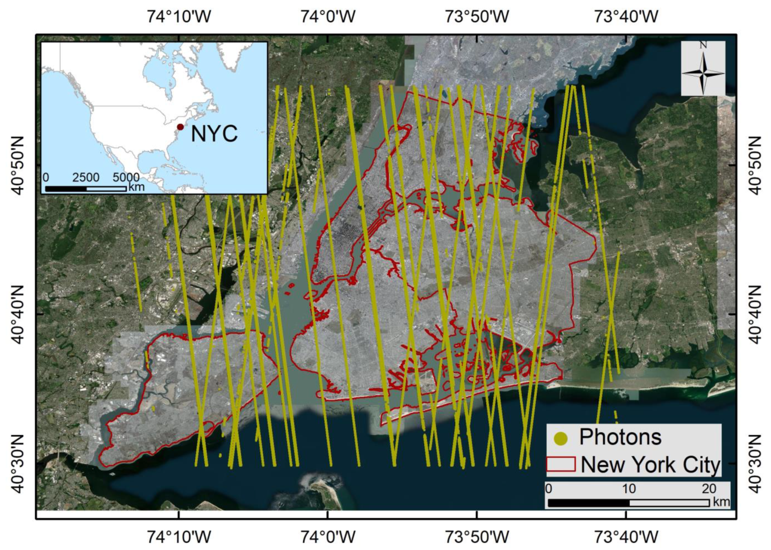
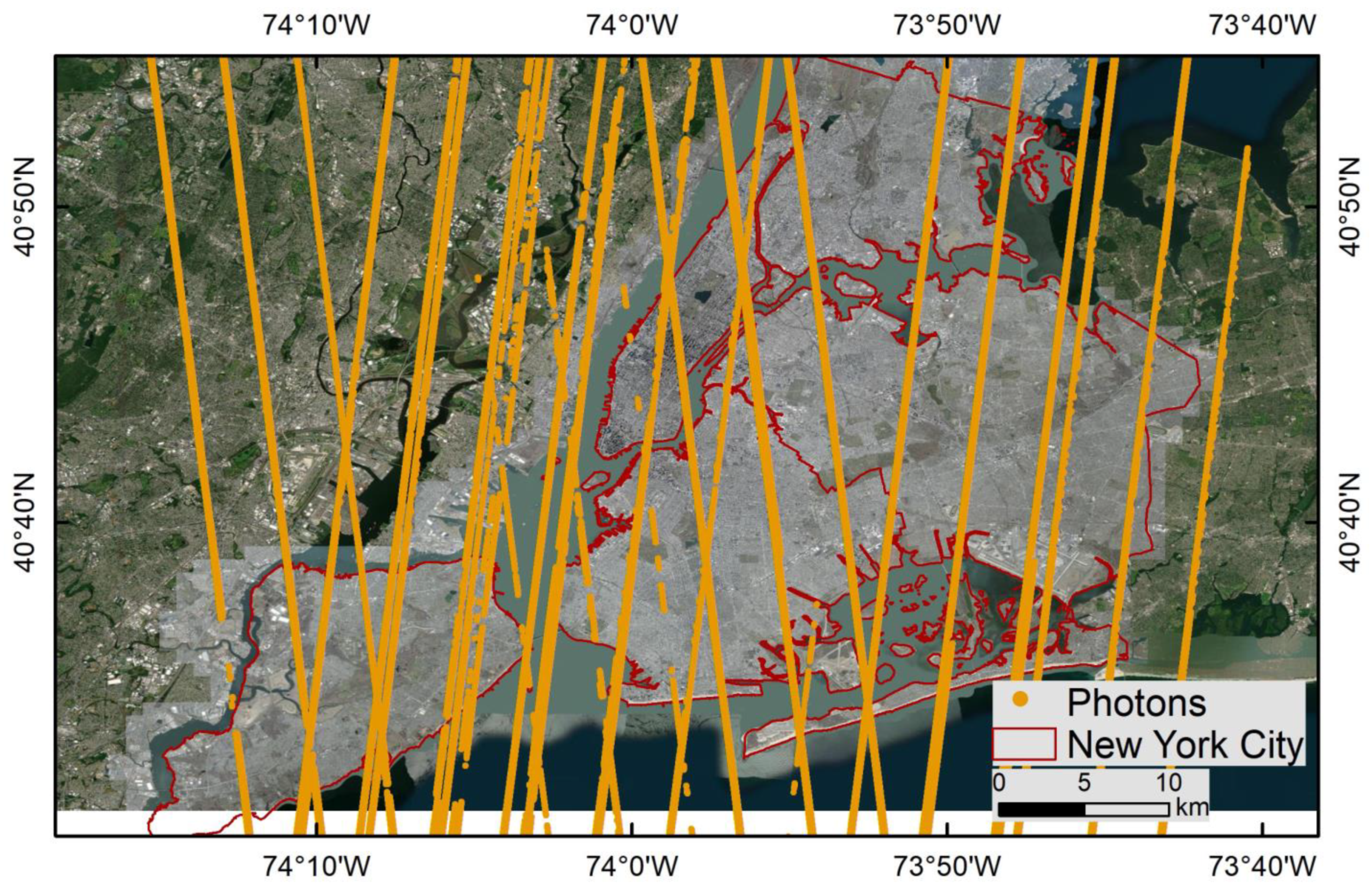
2.1. Study Area

New York City is one of the largest and most important cities in the world, located on the east coast of the United States. With a population exceeding 8,335,897 people in 2022, it is the most populous city in the US [42]. It had a gross regional product of USD 1514 billion in 2021, ranking first in the world [43]. The city covers an area of 300.45 square miles and comprises five boroughs: Manhattan, Brooklyn, Queens, the Bronx, and Staten Island [42]. Each borough has its unique character, architecture, and urban landscape. From the bustling streets and towering skyscrapers of Manhattan to the tree-lined avenues and brownstones of Brooklyn, the city’s diversity is reflected in its boroughs. As of 2018, there were over 1.07 million buildings in New York City, covering approximately 65% of the total area. This was calculated from building footprint data available at https://data.cityofnewyork.us/Housing-Development/Building-Footprints/nqwf-w8eh (accessed on 1 November 2023). Given that the accuracy of building height estimation is influenced by factors such as the environment, pattern, and height of a building, it becomes necessary to consider a greater number of factors in complex environments. New York City, with its rich architectural types, patterns, and heights, serves as an ideal location for experimental study. The intricate and diverse environment of the city ensures that the used methods are tested under realistic and challenging conditions, ultimately enhancing their reliability and generalizability. Figure 1 shows the satellite image of the study area overlaid with multiple beams of the ICESat-2 ground tracks. By establishing a high-precision building height estimation approach in NYC, the compatible model can be applied to various environments and has potential applications for other cities worldwide.

2.2. Data

2.2.1. ICESat-2/ATLAS

The ICESat-2 (Ice, Cloud, and Land Elevation Satellite 2) is a satellite mission launched by NASA (National Aeronautics and Space Administration) in September 2018 [44], equipped with the Advanced Terrain Laser Altimeter System (ATLAS) as its primary instrument. ATLAS uses laser pulses to measure the height of ice caps, glaciers, sea ice, and vegetation canopies on Earth’s surface with unprecedented precision. The ICESat-2 mission data are available to researchers and the public through the National Snow and Ice Data Center (NSIDC, https://nsidc.org/data/icesat (accessed on 1 October 2023)), which currently offers 21 products in 3 levels, including ATL01-21, stored in HDF5 (Hierarchical Data Format version 5) file format. For this study, we are using ATL03 production (Release 005, ATL03 V005), which contains global geo-located photon data comprising time, latitude, longitude, and elevation information for each photon event. This dataset allows us to extract and analyze the height of buildings in New York City.

2.2.2. Building Footprints NYC

Building Footprints NYC is a joint project between the New York City Department of Information Technology and Telecommunications (DoITT), the Department of Buildings (DOB), and the Department of City Planning (DCP). Its goal is to create a detailed map of New York City’s architectural footprint. The project provides information on the location, size, floors, height, number of stories, year of construction, and purpose of buildings in New York City in 2018. The data are available for download on NYC Open Data platform (https://data.cityofnewyork.us/Housing-Development/Building-Footprints/nqwf-w8eh (accessed on 1 November 2023)). We use this data to classify photons into candidate ground photons and building photons. The building extraction results are also verified by this dataset.

2.2.3. Landcover Raster Data (2010)

The high-resolution landcover raster data (2010) for New York City provides a detailed and accurate landcover dataset with 96% overall accuracy and 3-foot spatial resolution. It was created by the University of Vermont (UVM) spatial analysis laboratory using object-based image analysis (OBIA) technology and various remotely sensed and vector geographic information system (GIS) datasets. This data can be obtained from https://data.cityofnewyork.us/Environment/Landcover-Raster-Data-2010-3ft-Resolution/9auy-76zt (accessed on 4 November 2023). The landcover dataset includes seven categories: canopy, grass/shrub, bare earth, water, buildings, roads, and other paved surfaces. We utilize the canopy, grass, and other paved surfaces categories from this dataset for filtering ground points.

2.2.4. World Settlements Footprint (2019)

The World Settlements Footprint (WSF, 2019, https://geoservice.dlr.de/web/maps/eoc:wsf2019 (accessed on 10 November 2023)) is a dataset that provides a global representation of human settlements. It is derived from multi-temporal images captured by the Sentinel-1 and Sentinel-2 satellites in 2019. The images have a resolution of 10 m and an accuracy range of 83–89%. The WSF dataset specifically captures the distribution of buildings. In our analysis, we utilize the WSF data to calculate the density of buildings within a 100 m buffer zone surrounding the building profiles. This allows us to better understand the distribution and concentration of buildings in relation to the analyzed areas.

2.2.5. Digital Elevation Model (DEM)

To assess the accuracy of building height estimation across diverse terrains, we utilized the forest and buildings removed Copernicus DEM (FABDEM) dataset [45]. FABDEM employs a machine-learning technique called the random-forest regression model. This dataset is constructed by removing the height variations caused by buildings and trees from the Copernicus 30 m global (GLO-30) digital elevation model (CopDEM30) dataset.

2.2.6. Test Data

In order to evaluate the applicability of the method, this study opted to perform experiments in Beijing. The building footprint data utilized in the study were derived from network data in 2018 (https://www.dilitanxianjia.com/ (accessed on 1 December 2023)), with the number of floors serving as a means of verification. It was assumed that each floor corresponded to a height of 3 m. The land use data employed in the study were generated through a collaboration between the Environmental Systems Research Institute (ESRI), Impact Observatory, and Microsoft, utilizing Sentinel-2 satellite data with a resolution of 10 m [46].

2.3. Methods

The method for extracting building height using ATL03 photons and building footprint data involves three main stages: preliminary noise removal, extraction of ground and building photon, and accuracy assessment of height estimates. The methodological framework is illustrated in Figure 2.

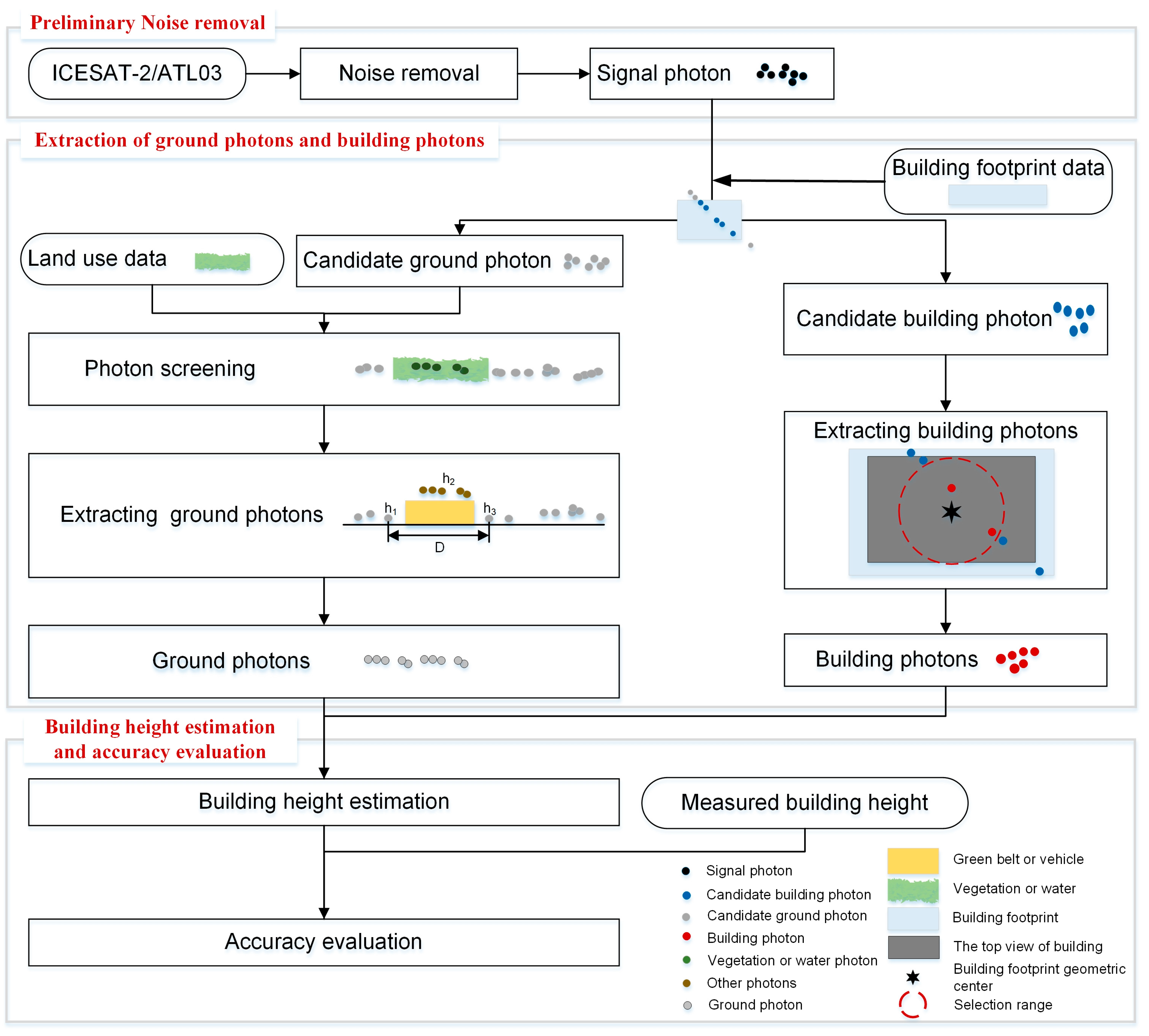
2.3.1. Preliminary Denoising

ATL03 V005 includes two parameters, photon quality (quality_ph) and photon signal confidence (signal_conf_ph), to distinguish between noise and signal photons [47]. These parameters indicate the quality and confidence level of each photon event selected as a signal per surface type (land, ocean, sea ice, land ice, and inland water). The “quality_ph” parameter has four possible values (0, 1, 2, and 3), representing nominal, possible_afterpulse, possible_impulse_response_effect, and possible_tep, respectively. The “signal_conf_ph” parameter has seven possible values (−1, −2, 0, 1, 2, 3, and 4), representing low to high signal confidence, accordingly.

Typically, only photons with quality_ph = 0 and signal_conf_ph = 3 or 4 of a land surface are retained as effective signal photons for further analysis. They are considered to be high-quality signal photons with a high likelihood of being actual signals.

2.3.2. Extracting Building Photons and Ground Photons

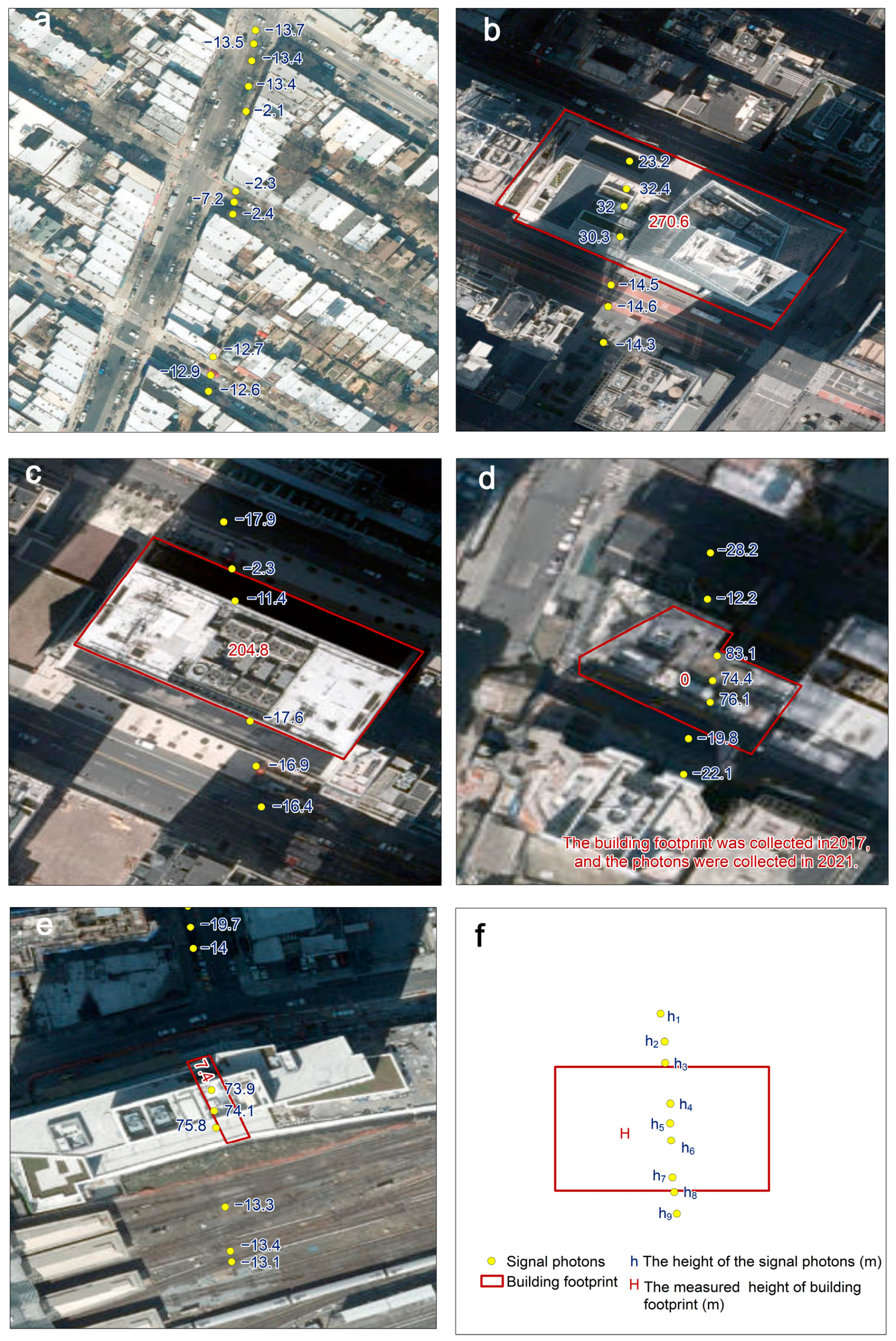
Building photons and ground photons can be obtained initially by classifying signal photons using building footprint data. However, accurately extracting building heights from these photons is challenging due to several issues that need to be addressed:

i.

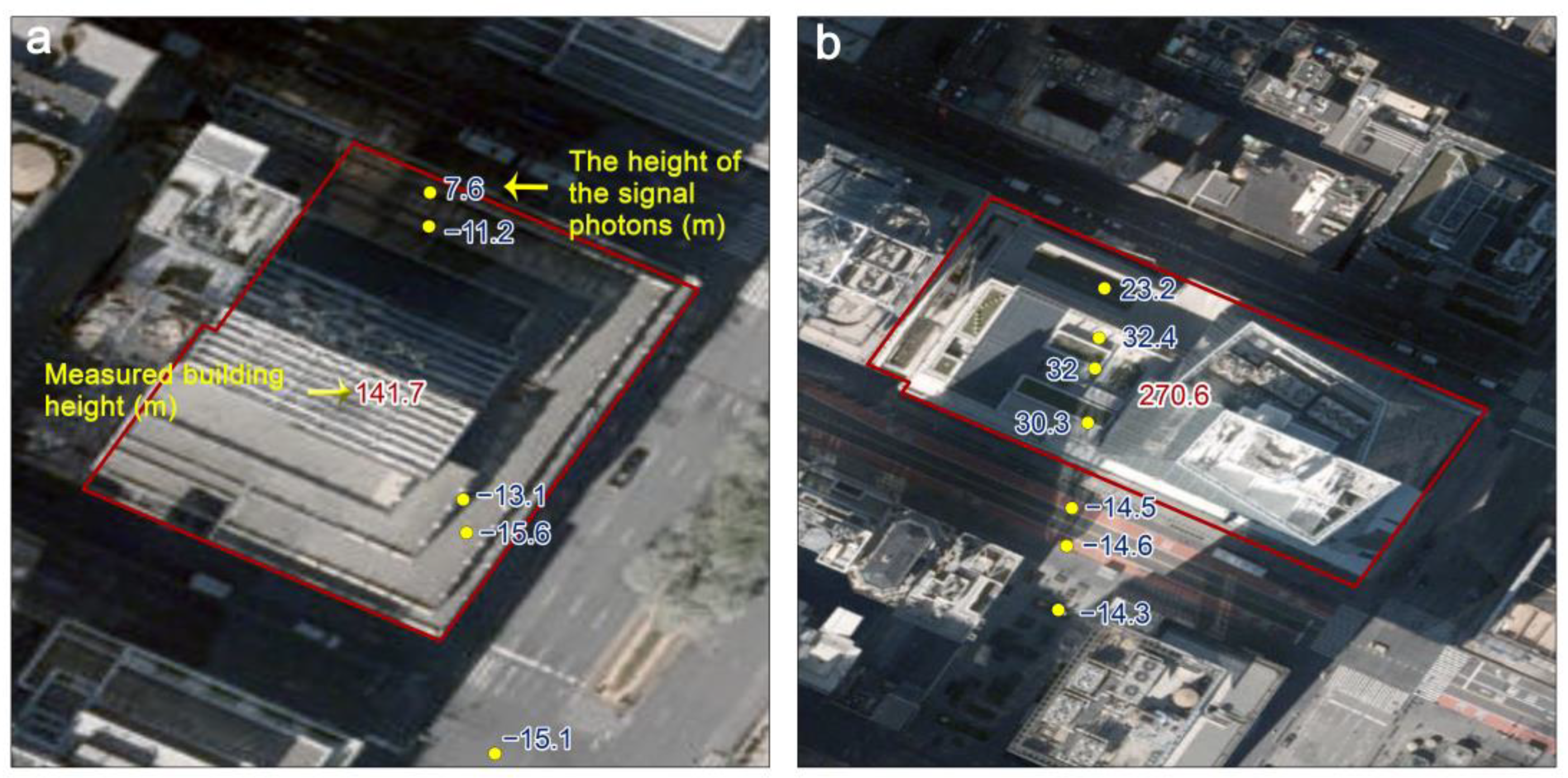
The height of ground photons may not reflect the true base-level height (net ground surface) of the building, leading to discrepancies in building height measurements (Figure 3a). For instance, ground photons may fall on vegetation, depression, or other artificial or natural objects, resulting in a building height that is either lower or higher than the actual building height.

ii.

Laser photons may not hit the highest point of the building, resulting in an inaccurate measurement of the building height (Figure 3b).

iii.

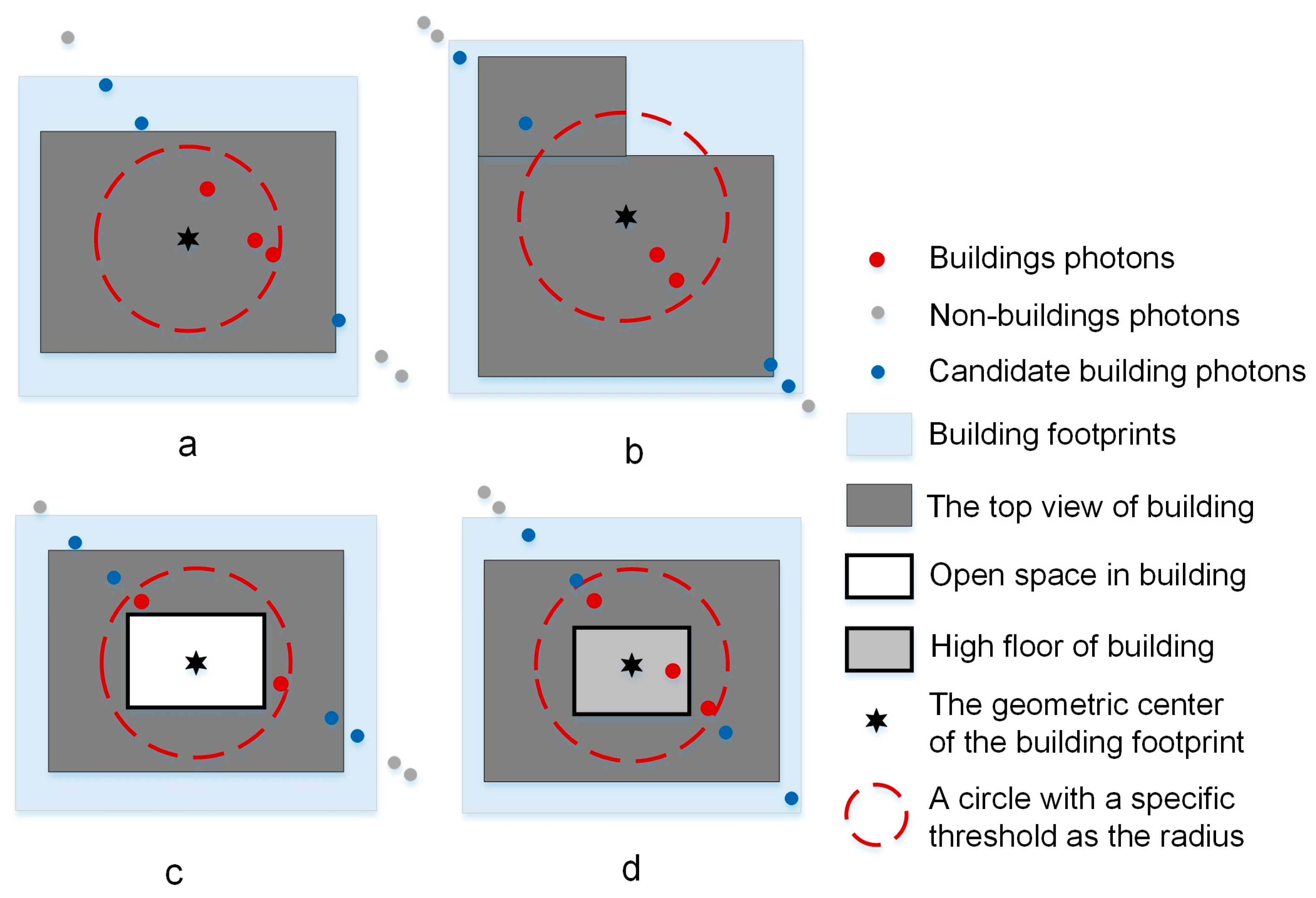
Building photons that fall on the edge of the building’s contour may not necessarily be located on the building itself (Figure 3c).

iv.

Discrepancies in building height measurements can arise due to mismatches between date of building construction, photon acquisition time, and building ground measurement time (Figure 3d). For example, if a building is under construction during field measurement but completed by the time the point cloud is acquired, the height recorded in the point cloud may be greater than the height measured on-site.

v.

Other issues include errors in manual data processing of building footprint data (Figure 3e).

To improve the accuracy of building height measurements, further processing of ground and building points is necessary due to the issues mentioned above. This involves three steps:

(1)

Filtering ground photons

The obtained ground photons from building footprint data classification may not accurately represent the reference heights of adjacent buildings due to inaccuracies as described in problem i above. To solve this problem, we performed three operations:

• Sifting ground photons using landcover raster data to remove points that fell on tree canopy, grass/shrub, and other paved surfaces.
• Applying a density-based radius filtering method with a range of 5 m and at least 3 supporting photons within this range to remove outliers while retaining useful information.
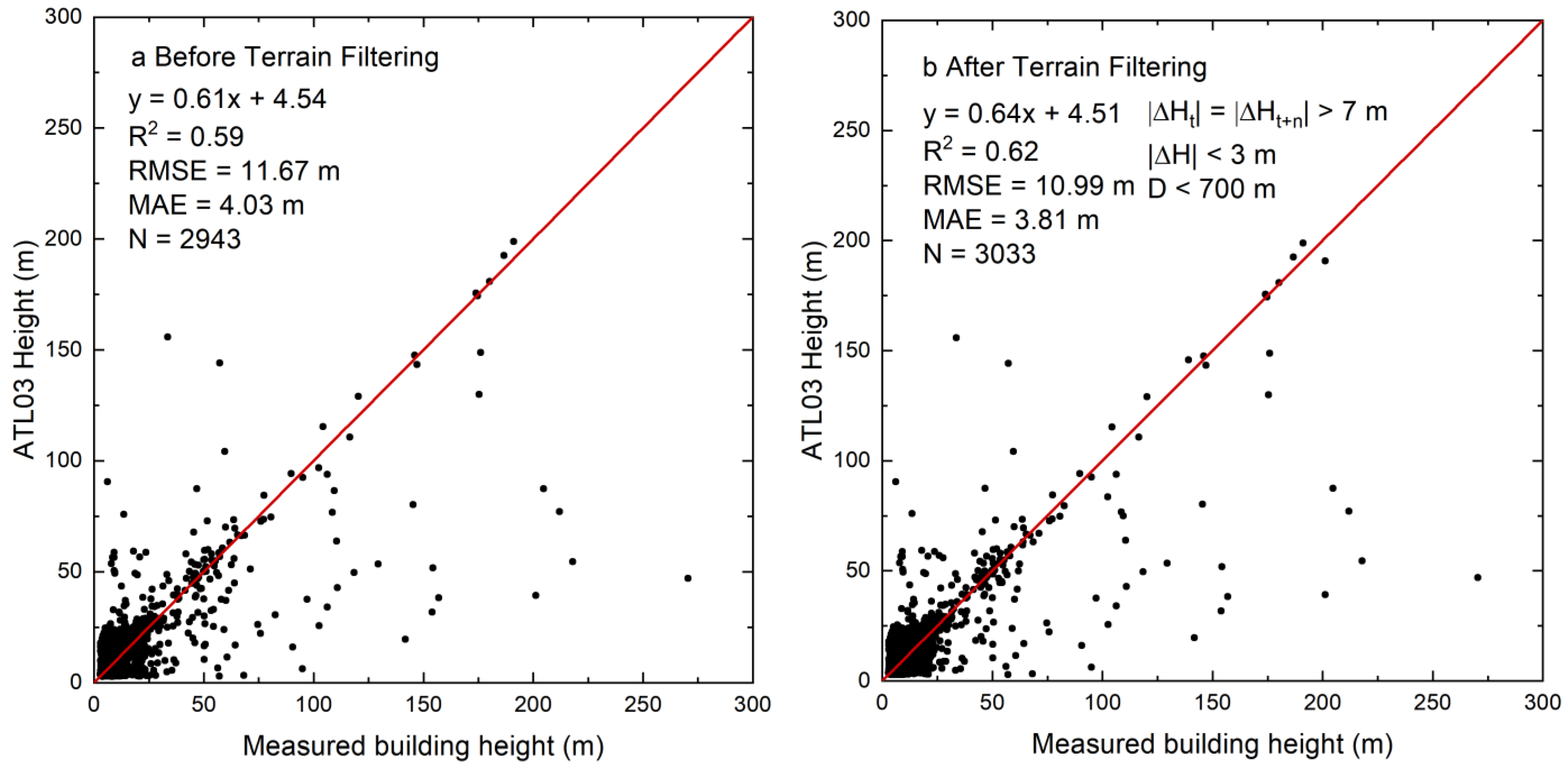
• Calculating the height difference between adjacent photons along the track direction to remove abnormal ground relief. If the absolute value of the height difference between photon t and its next photon was greater than h meters (Formula (1), |∆H_t| > h), the position of the photon t was considered the starting point of terrain relief. Along the track direction, when photon t + n encountered an absolute value of height difference greater than h meters again (Formula (2), |∆H_t+n| > h), the position of the photon t + n was considered as the end point of terrain relief. The distance (D, Formula (4)) between photon t and photon t + n and the height difference between photon t and photon t + n (∆H, Formula (3)) were calculated. If the absolute value of the height difference was less than n meters and the distance was less than m meters (|∆H| < m, D < d), the terrain relief was considered abnormal, and all photons between photon t and photon t + n were removed (Formula (5)).

$$\Delta {\mathrm{H}}_{\mathrm{t}}={\mathrm{H}}_{\mathrm{t}}-{\mathrm{H}}_{\mathrm{t}+1}$$

(1)

$$\Delta {\mathrm{H}}_{\mathrm{t}+\mathrm{n}}={\mathrm{H}}_{\mathrm{t}+\mathrm{n}}-{\mathrm{H}}_{\mathrm{t}+\mathrm{n}+1}$$

(2)

$$\Delta \mathrm{H}={\mathrm{H}}_{\mathrm{t}+\mathrm{n}+1}-{\mathrm{H}}_{\mathrm{t}}$$

(3)

$$\mathrm{D}=\sqrt{{\left({\mathrm{X}}_{\mathrm{t}+\mathrm{n}}-{\mathrm{X}}_{\mathrm{t}}\right)}^2+{\left({\mathrm{Y}}_{\mathrm{t}+\mathrm{n}}-{\mathrm{Y}}_{\mathrm{t}}\right)}^2}$$

(4)

$$(\left|\Delta {\mathrm{H}}_{\mathrm{t}}\right|>\mathrm{h})\cup (\left|\Delta {\mathrm{H}}_{\mathrm{t}+\mathrm{n}}\right|>\mathrm{h})\cup (\left|\Delta \mathrm{H}\right|<\mathrm{m})\cup (\mathrm{D}<\mathrm{d})$$

(5)

The notation used in these formulas includes:

• t: the index of the t-th photon along the track;
• t + n: the index of the (t + n)-th photon along the track;
• H_t: the height of the t-th photon;
• ∆H_t: the height difference between the t-th and (t − 1)-th photons along the track;
• ∆H: the height difference between the (t + n)-th and t-th photons along the track;
• X_t: the abscissa of the t-th photon under the UTM projection;
• Y_t: the ordinate of the t-th photon under the UTM projection;
• D: the Euclidean distance between the t-th and (t + n)-th photons along the track;
• h, m, and d: constant variable.

To determine the optimal values of h, m, and d, we conducted an experiment using a control variable method, randomly selecting 50 tracks that passed through the urban area of New York City (Figure A1). Firstly, we held the d constant and adjusted the values of h and m (

Table 1. Variable threshold (h, m) setting during filtering ground photons.

h (m) (|∆Ht| and |∆Ht+n| > h)	m (m) (|∆H| < m)	d (m) (D < d)
2	5	1000
2	7	1000
2	10	1000
2	13	1000
2	16	1000
3	5	1000
3	7	1000
3	10	1000
3	11	1000
3	13	1000
3	16	1000
4	10	1000
5	7	1000
5	10	1000
5	13	1000
5	16	1000

). We then selected the optimal values of h and m (h_best and m_best) by comparing the resulting accuracy in estimated building height. Once the optimal values of h and m were determined, we held them constant and adjusted the d (

Table 2. Variable threshold (d) setting during filtering ground photons.

h (m) (|∆Ht| and |∆Ht+n| > h)	m (m) (|∆H| < m)	d (m) (D < d)
hbest	mbest	100
hbest	mbest	300
hbest	mbest	500
hbest	mbest	700
hbest	mbest	900
hbest	mbest	1000
hbest	mbest	1100
hbest	mbest	1300

). We selected the final value of d based on the resulting change in precision. This allowed us to evaluate the impact of each parameter on building height accuracy while holding other factors constant.

(2)

Filtering building photons

Accurate placement of building photons is indeed crucial for successful building height extraction and avoiding problems ii and iii. The presence of diverse building types (Figure 4) and non-uniform photon distribution on the ground objects (Figure 3) can pose challenges in this process. To address this, the following method is employed to ensure that the identified building points correspond to actual buildings. Regardless of the shape of the building, the distance between the building photons and the geometric midpoint of the building footprint is calculated. Photons within a distance of less than a certain threshold are retained, while those outside this range are removed (Figure 4).

To optimize the accuracy of building extraction and select the most suitable approach, different candidate thresholds are prepared and tested, ranging from 0 to 12/12 of the minimum building footprint width. The optimal threshold is determined by balancing the accuracy and number of buildings extracted. This iterative process helps improve the accuracy of building extraction and ensures the amount of extracted building heights.

(3)

Building height estimation

The building height estimation process involves using the nearest-neighbor algorithm to predict and reconstruct the ground surface and calculate the difference between building photons and the ground as the height of the building. However, problems ii and iv persisted despite this method. To address these issues, two additional operations were implemented based on the actual situations.

The highest point of the remaining building photons within each filtered building contour is assumed to represent the building’s height. This is on the assumption that the measured height of a building is generally the highest height, and all remaining building photons are valid and reliable after filtering. This is common especially when the top of a building is not flat.

To avoid errors caused by ground photons being misclassified as building photons and resulting in a building height below 2.8 m, a condition is set that the point cloud building height must be greater than 2.8 m. This threshold is based on the fact that typically the lowest roof height is around 2.8 m, ensuring that only valid building points are included in the calculation of building height.

2.3.3. Accuracy Evaluation

To ensure accuracy in the comparison of building heights, we took into account that the building footprint data included structures that were planned but not yet constructed. Consequently, these buildings were measured with a height of less than 2.8 m (Figure 3d). In order to mitigate the height error caused by the time difference, we removed the data corresponding to measured buildings with a height below 2.8 m. This step helped eliminate the potential impact of incomplete construction on the height comparison between the ATL03 building data and the measured building data.

The accuracy of the ATL03 building height extraction was evaluated using several primary indices including determination coefficient (R²), root mean square error (RMSE), mean absolute error (MAE), and bias. The R² was used to measure the goodness-of-fit between the predicted and measured building heights. A higher R² value indicates a better fit between the predicted and measured values. RMSE is another index used to evaluate the accuracy of the predicted building heights. RMSE measures the average deviation between the predicted and measured values. A lower RMSE value indicates a higher degree of accuracy. MAE is the absolute average difference between the predicted and measured values. It provides an indication of the overall magnitude of the prediction errors, regardless of their direction. A lower MAE value also indicates a higher degree of accuracy. Bias represents the systematic difference between the predicted and measured values. A positive bias indicates that the predicted values are consistently higher than the measured values, while a negative bias indicates the opposite. Bias can be calculated as the difference between the mean predicted and measured values.

$${\mathrm{R}}^2=1-\frac{{\displaystyle \sum {\left({\mathrm{H}}_{\mathrm{A}\mathrm{T}\mathrm{L}03}-{\mathrm{H}}_{\mathrm{O}}\right)}^2}}{{\displaystyle \sum {({\mathrm{H}}_{\mathrm{A}\mathrm{T}\mathrm{L}03}-\overline{{\mathrm{H}}_{\mathrm{O}}})}^2}}$$

(6)

$$\mathrm{R}\mathrm{M}\mathrm{S}\mathrm{E}=\sqrt{\frac{{\displaystyle \sum {\left({\mathrm{H}}_{\mathrm{A}\mathrm{T}\mathrm{L}03}-{\mathrm{H}}_{\mathrm{O}}\right)}^2}}{\mathrm{n}}}$$

(7)

$$\mathrm{M}\mathrm{A}\mathrm{E}=\frac{{\displaystyle \sum \left|{\mathrm{H}}_{\mathrm{A}\mathrm{T}\mathrm{L}03}-{\mathrm{H}}_{\mathrm{O}}\right|}}{\mathrm{n}}$$

(8)

$$\mathrm{B}\mathrm{i}\mathrm{a}\mathrm{s}=\frac{{\displaystyle \sum ({\mathrm{H}}_{\mathrm{A}\mathrm{T}\mathrm{L}03}-{\mathrm{H}}_{\mathrm{O}})}}{\mathrm{n}}$$

(9)

The notation used in these formulas includes:

• H_ATL03: estimated building heights based on ATL03 data;
• H_O: observed building height;
• n: number of variables.

In summary, the evaluation of accuracy indices provides useful insights into the performance of the proposed building height extraction method using ATL03 data. The results can help identify any limitations or issues related to the method, as well as suggest possible improvements for future research.

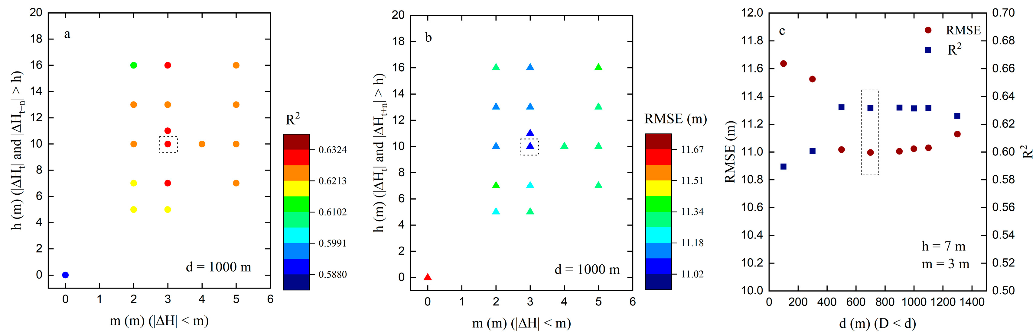
2.4. Parameter Sensitivity Analysis

In this model, the accuracy of building height extraction can be influenced by the parameter thresholds h, m, and d in the ground point filtration process, as well as the parameter thresholds p in the building photon selection process. To assess the impact of threshold changes on the results and evaluate its scalability, we conducted a single-factor sensitivity analysis on the accuracy evaluation index RMSE of the research object.

In this analysis, we kept all other factors constant and only modified one single factor by either 30% or 33% at each time. We then observed the change in the accuracy evaluation index RMSE and calculated the sensitivity of each parameter threshold using Formula (10). The sensitivity coefficient indicates the degree of sensitivity of the variable to the precision evaluation index RMSE. A higher sensitivity coefficient implies a greater sensitivity of the variable to the RMSE.

$$\mathrm{S}\mathrm{V}\mathrm{F}=\frac{\Delta \mathrm{R}\mathrm{M}\mathrm{S}\mathrm{E}}{\Delta \mathrm{F}}$$

(10)

where SVF represents the sensitivity coefficient of the evaluation index to the uncertainty factor F, ΔRMSE represents the percentage change in the evaluation index RMSE when the uncertainty factor F changes by ΔF, and ΔF represents the rate of change (%) of the uncertainty factor F that is being examined.

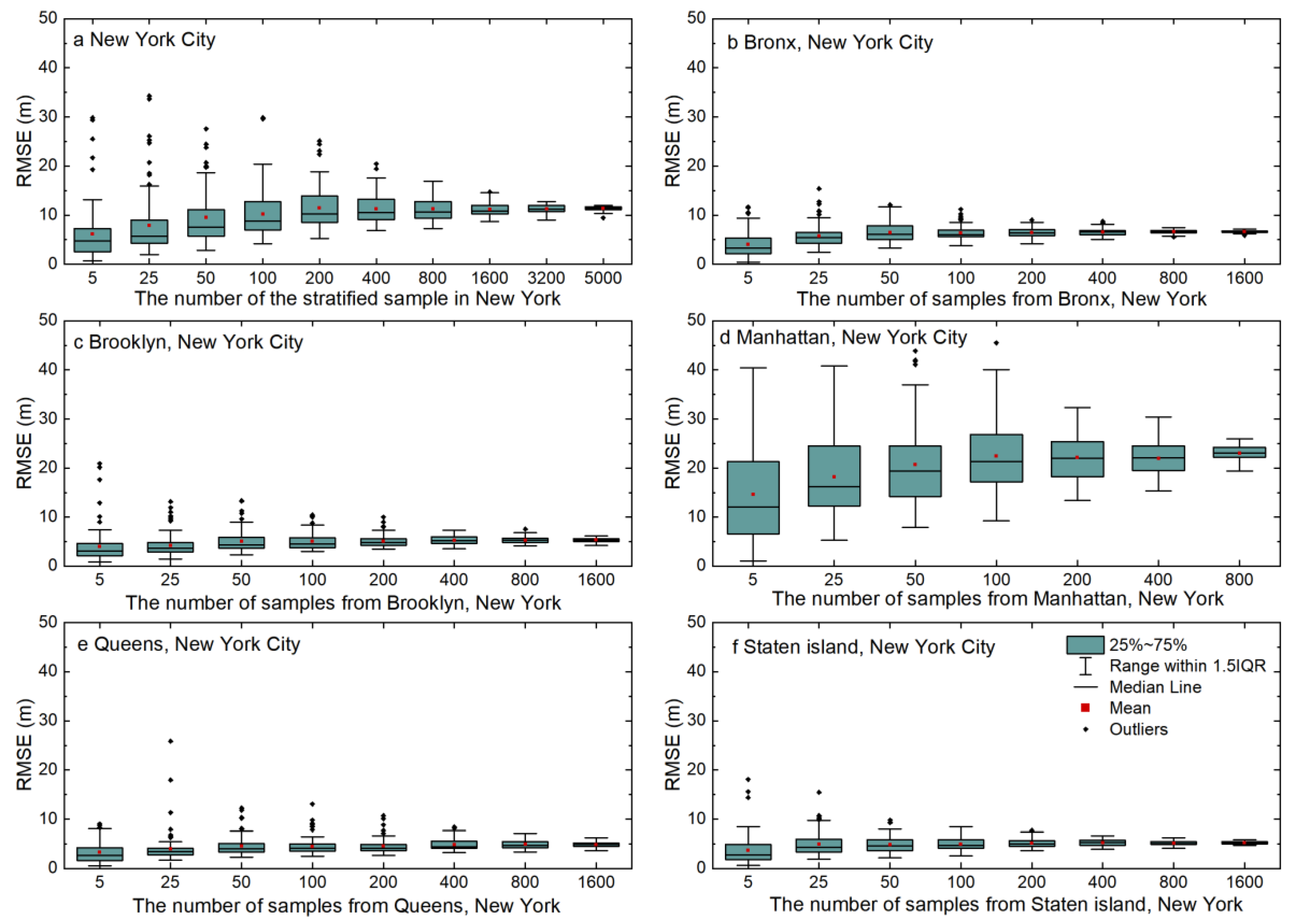
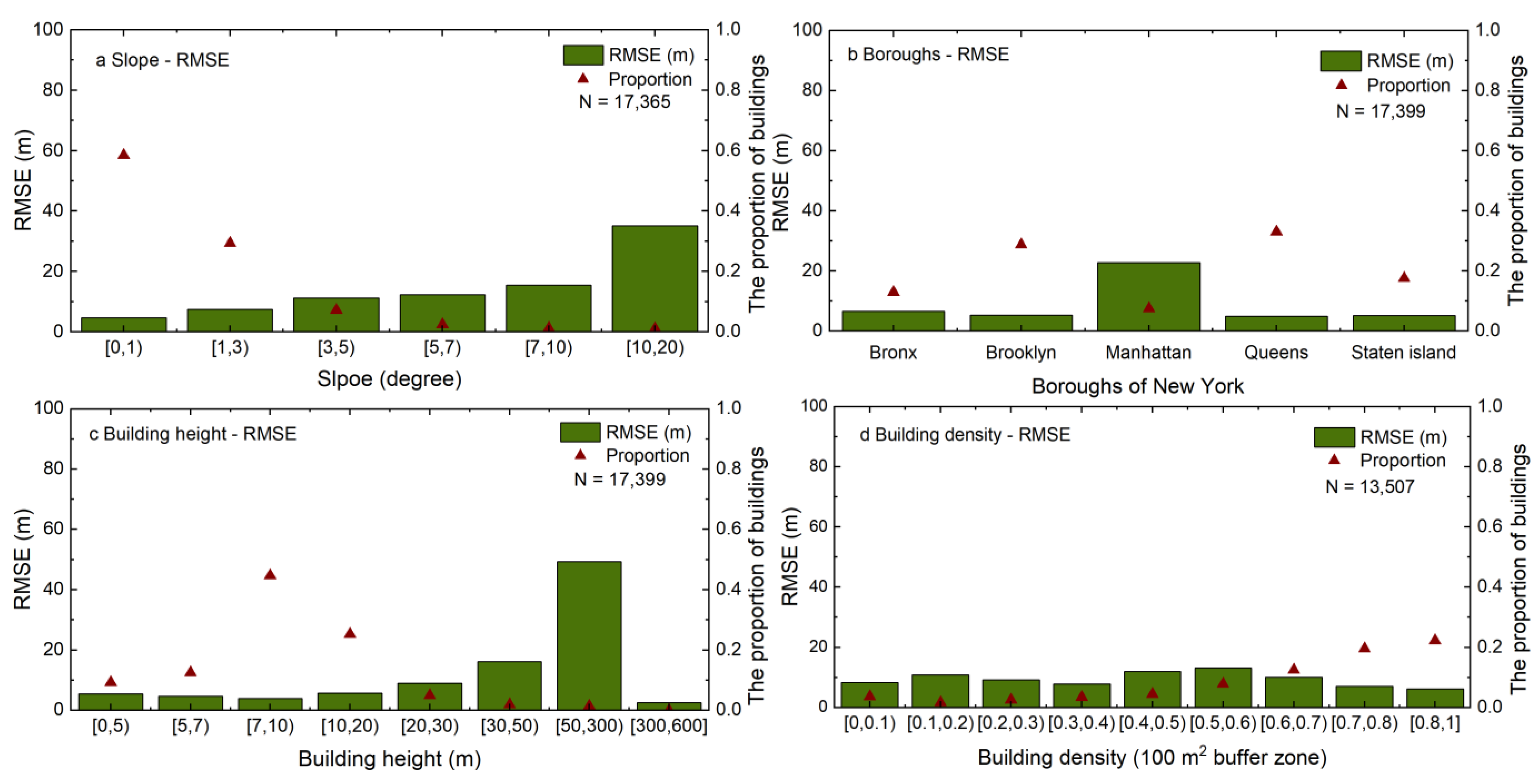
2.5. Analysis of the Influence of Building Number and Building Height Estimation Accuracy

To analyze the influence of the number of buildings on accuracy, we conducted an analysis using a random sampling method with 100 iterations. Two sampling methods were employed:

• Analysis based on New York City’s boroughs: We analyzed the relation between building number and estimation accuracy within each borough.
• Mixed analysis of all New York City boroughs: In each iteration, a fixed number of buildings were selected from each district for the purpose of spatially representativeness, and they were aggregated together to compute an overall accuracy.

3. Results and Discussion

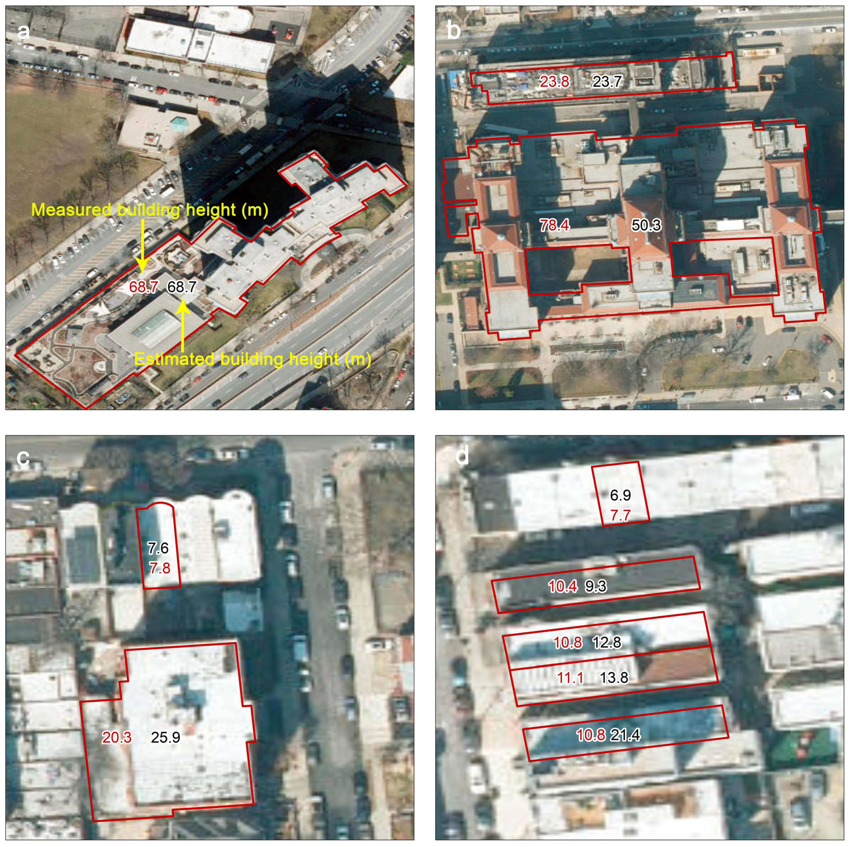
3.1. Building Height Estimation

This study used ATL03 data to extract the heights of 17,399 buildings in New York City and verified the results with the building heights in Building Footprints NYC. Figure 5a shows a linear relationship between the estimated building height from ATL03 and the measured building height from Building Footprints NYC, with an RMSE of 8.1 m and MAE of 3 m. The majority of the buildings (71%) had an absolute difference of less than 3 m, while 93% had a difference of less than 10 m. Furthermore, 69% of the buildings demonstrate a relative error of less than 30% (Figure 5b).

Moreover, this study delved into buildings displaying significant disparities between the estimated and measured heights. This investigation revealed that such differences primarily stem from two underlying issues (Figure 5c,d). The first issue relates to the fact that the ATL03 signal photon does not always align with the highest point of the building (Figure 5c). This is an inherent limitation of satellite-based laser data, which can only provide the height of the photon along its orbital path. Efforts have been made to address this by extracting the maximum height of the building from the available data. The second issue arises from potential recording errors in building footprint during the manual data collection process, which are challenging to completely eliminate (Figure 5d). Buildings in some areas may have changed due to time, but they are probably not updated timely.

Overall, the study demonstrates that the proposed method effectively extracts building heights using ATL03 data.

3.2. The Instability of Model Parameters

3.2.1. Parameters of Ground Photon Screening

Variations in terrain can have a significant impact on the accuracy of building height estimation, especially in regions with high relief. This is because the elevation of surrounding ground photons can influence the accuracy of building height estimates. Terrain fluctuation caused by vegetation or other nearby structures can also create more than 10-m differences in ground height of the adjacent streets, resulting in building height estimation errors (Figure 3a–c). To address this issue, we filter ground points to remove abnormal terrain relief.

It has been observed that the selection of the threshold values has a significant impact on the results obtained. Specifically, when the D < 1000 m, the best results were obtained when |∆H_t| and |∆H_t+n| > 10 m, and |∆H| < 3 m, yielding an RMSE of 11.02 m and an R² of 0.63 (Figure 6a,b). By keeping the same threshold condition of |∆H_t| and |∆H_t+n| > 10 m, and |∆H| < 3 m, and adjusting the value of d, the best result was achieved with the D < 700 m, yielding an RMSE of 10.99 m and an R² of 0.63 (Figure 6c).

Removing abnormal terrain fluctuations improved the results, increasing the R² by 0.03, decreasing the RMSE by 0.68 m, and increasing the number of estimated buildings by 90 (Figure 7). However, some abnormal points remained due to inconsistencies in data between ATL03 photon height and measured data (Figure 7 and Figure A2). Extraction of buildings on complex terrain is challenging and has practical limitations.

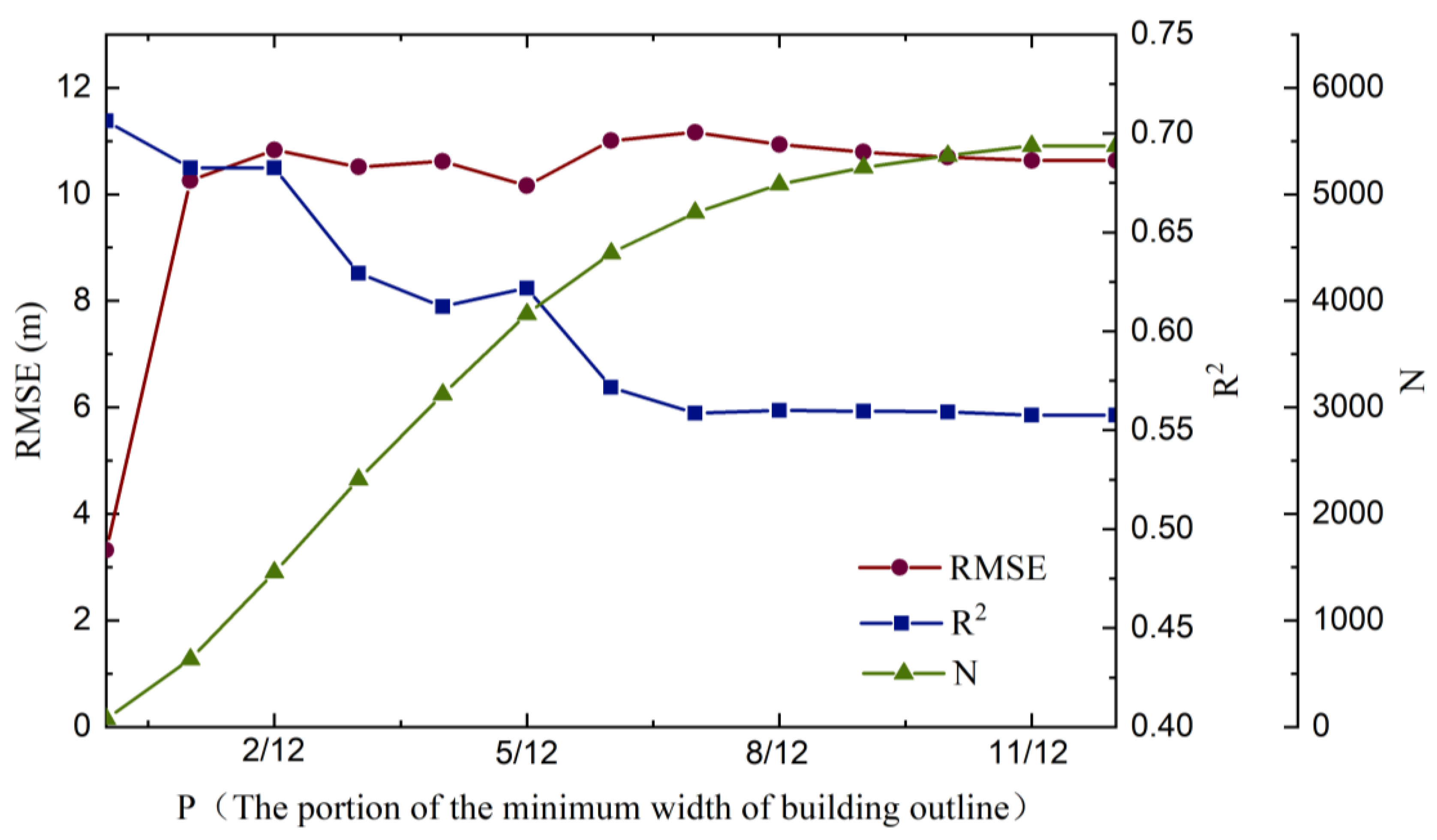
3.2.2. Parameters of Building Photon Screening

Measurement tools and computational limitations methods can cause building silhouettes to not fully overlap with the actual building, leading to errors in classification and height extraction (Figure 3d,e). To reduce these errors, we used statistical techniques to filter the data by calculating the distance between ICESat-2/ATL03 building photons and the building footprint’s geometric center. We reserved appropriate building photons using various distance thresholds and determined the building extraction accuracy (Figure 8). Lowering the distance threshold and only keeping the central photons increased extraction accuracy but reduced the number of extracted buildings significantly. When the distance threshold reduced from 1 to 0, the RMSE of building extraction accuracy increased by 7.4 m, and R² decreased by 0.15. However, the number of extracted building heights reduced dramatically by 98.6% (from 5456 to 75). It should be noted that when there is a building with a ring structure, choosing a smaller threshold value may cause the retained building photons not to fall on the actual building, resulting in incorrect extracted building height. Therefore, it is crucial to choose a reasonable distance threshold to balance the accuracy and number of remaining buildings. A threshold of 5/12 of the minimum building footprint width was finally chosen for a balance between accuracy and the number of extracted buildings, resulting in an RMSE of 10.1 m, an R² of 0.62, and an N of 3877 (Figure 8). It is important to note that the results also have the issues of data consistency raised in question v.

3.2.3. Variable Sensitivity Analysis

Based on the single-factor sensitivity analysis, it was found that the accuracy evaluation index RMSE is most sensitive to the threshold value p, moderately sensitive to threshold h and d, and least sensitive to the m value (

Table 3. Sensitivity coefficient of RMSE to parameters. m, h, d, and p are the parameter thresholds in the model that affect RMSE. ΔF represents the rate of change of the parameter threshold. ΔRMSE represents the rate of change of RMSE when F changes ΔF. SAF is the sensitivity coefficient.

Variables	m		h		d		p
ΔF	33%	−33%	30%	−30%	30%	−30%	33%	−33%
ΔRMSE	2.20%	0.80%	1.40%	2.20%	1.00%	2.40%	−0.60%	−3.50%
SAF	0.07	−0.02	0.05	−0.07	0.03	0.08	−0.02	0.11

). This implies that the error between the true value and the estimated value is primarily influenced by the value of p. Lowering the threshold value p results in a decrease in the RMSE, as the error is reduced. However, this also leads to a decrease in the number of retained building photons and the number of extracted building heights (Figure 8). Additionally, when complex building structures appear, selecting a smaller threshold value p may cause the building photons in the selected area to not align accurately with the actual building. Consequently, the true building height cannot be obtained in such cases. On the other hand, increasing the threshold value p leads to the selection of more building photons, which may improve the RMSE. However, if the threshold value p becomes too large, problem iii arises (Figure 3c). In this case, the filtered building photons may fall on the contour edge of the building, such as vegetation, rather than on the actual building. As a result, there are more significant differences between the estimated building height and the true value, leading to a decrease in the coefficient of determination (R²) and an increase in the RMSE (Figure 8). It is evident that the threshold value p significantly affects both the quantity and quality of the screened building photons. Therefore, careful consideration should be given to selecting an appropriate threshold value p. Balancing the trade-off between reducing the RMSE and ensuring accurate building height estimation is crucial.

Threshold values for h, d, and m play a crucial role in the filtration of ground points. These thresholds are essential in identifying and filtering out ground points that may be located in depressions, vegetation, or viaducts. The presence of these points can distort the surface of the terrain, resulting in inaccurate extraction of building height. Among these thresholds, the threshold value “d” determines the degree to which abnormal relief in the terrain is considered. If the threshold value “d” is set too low, it may fail to identify similar points located on vegetation or other objects as abnormal. Conversely, if the threshold value “d” is set too high, it may mistakenly flag actual topographic relief as abnormal, leading to erroneous building height extraction and a higher RMSE. The threshold value “h” determines the minimum height difference between adjacent ground points that is recognized as an anomaly. Similarly, the threshold value “m” determines the threshold for the termination of a complete anomalous topographic relief. Setting excessively large or small values for h and m can introduce errors in ground surface fitting and increase the RMSE of extracted building height.

3.3. The Expansibility Analysis of the Model

In order to analyze the scalability of the method in different regions, we added a test in Beijing. A typical core urban area within the second ring road in Beijing was chosen as our testing area (Figure A3), and a total of eight buildings were randomly selected for estimation using the data from two tracks of ATL03. The verification data used were the number of building floors from the land register, and it was assumed that each building had a height of 3 m (

Table 4. Accuracy of height estimation of eight buildings in Beijing.

Building No.	Measured Building Height (m)	Estimated Building Height (m)	Absolute Error (m)	Relative Error (%)
1	3	2.96	0.04	1
2	3	3.25	−0.25	8
3	6	6.28	−0.28	5
4	18	18.75	−0.75	4
5	3	3.27	−0.27	9
6	3	4.12	−1.12	37
7	3	4.11	−1.11	37
8	66	68.13	−2.13	3

). The results showed that for both high-rise and low-rise buildings, the absolute error was less than 2.1 m, and the relative error was less than 37%.

Additionally, we calculated the accuracy distribution of building height estimates in New York City based on factors such as slope, region, building density, and height (Figure 9). The analysis revealed several interesting findings. Firstly, it was observed that the majority of buildings (10,172) were situated on terrain characterized by a slope of less than 1 degree, accounting for 58% of the total number. These buildings had the highest accuracy, with an RMSE of 4.7 m (Figure 9a). As the slope increased, the number of buildings decreased along with the accuracy.

Furthermore, the study evaluated the building height estimation accuracy in the five administrative regions of New York individually (Figure 9b). The Queens area exhibited the highest accuracy, with an RMSE of 4.9 m. Notably, the buildings in the Queens area accounted for approximately 33% of the total number of buildings in New York. On the other hand, the Manhattan area had the lowest accuracy, with an RMSE of 22.7 m and comprised 7% of the total number of buildings. The low accuracy in this area can be attributed to the presence of numerous tall buildings. Accurate height estimation relies on the ATL03 signal photon accurately hitting the highest point of a building, which is challenging to guarantee in such cases.

In addition, the study examined the height estimation accuracy of buildings with different heights and densities (Figure 9c,d). It was found that the accuracy decreased with increasing building heights. Buildings below 20 m had higher accuracy, with an RMSE of less than 6 m, and accounted for 91% of the total number. Among these, buildings between 7 and 10 m had the highest accuracy, reaching 3.9 m. The extraction accuracy of different building densities also varied significantly. Moreover, the accuracy of height extraction varied significantly based on building density. Interestingly, the highest density corresponded to the best accuracy, with buildings having a density greater than 0.7 within 100 m² accounting for 42% of the total number and an RMSE below 7 m.

Upon analyzing the complexity of buildings and the accuracy of building height estimation, we have discovered that the accuracy of height estimation is not necessarily dependent on the building structure. Both complex and simple buildings exhibit a mix of accurate and inaccurate height estimations (Figure 10). However, it is important to note that the estimation error may be more pronounced for high-rise buildings with complex structures. This is primarily due to the difficulty in ensuring that the photon accurately falls on the highest point of such intricate buildings.

It is worth noting that the number of buildings does impact the estimation of building height (Figure A4). When the number of buildings is small, the estimated accuracy may exhibit large instability, but the average accuracy tends to be high. However, as the number of buildings increases sufficiently, the estimated accuracy of buildings becomes more stable, albeit with a lower average accuracy.

As a result, our method demonstrates excellent scalability in regions characterized by gradual changes in gradient, dense buildings, and low building heights. However, challenges may arise in areas with complex and tall building structures. This is predominantly attributed to the positioning of ATL03 photons, which are utilized for extracting building height. To mitigate these challenges, it is crucial to employ multiple tracks that sweep through the area, thereby maximizing the photon coverage and enhancing the accuracy of height estimation.

3.4. Comparing to Existing Method of Building Height Based on ICESat-2 Data

To further evaluate the performance of our method, we compared it with existing building height estimation methods based on ICESat-2 data [21,35,40,41,48] (

Table A1. Comparison of building height extraction methods based on ICESat-2 data.

Study	Study Area	The Number of Buildings	Reference Sources	Precision
This study	New York, USA	17,399	BuildingFootprints NYC	RMSE = 8.1 m, MAE = 3 m
Lao’s study [35]	Haidian, Beijing, China	75	The field measurement used Rigel VZ-1000 laser scanning system	RMSE = 0.35–0.45 m
Dandabathula’s study [40]	Jaipur city, India	10	The field measurement used zero-elastic carpenter’s thread (scientific grade)	MAE = 0.13 m
Goud and Bhardwaj’s study [41]	Hyderabad, Paris and Vancouver	30	Determined the number of floors for each sample building utilizing Google Images and Google Earth Pro	RMSE = 2.04 m
Wu and Zhao’s study [48]	Wujiaochang in the Yangpu District of Shanghai, China	468	The Digital Surface Model (DSM) data provided by Shanghai Surveying and Mapping Institute	RMSE = 6.75 m, MAE = 4.70 m
Wu and Zhao’s study [21]	The city center of Shanghai, China	1176	The Digital Surface Model (DSM) data provided by Shanghai Surveying and Mapping Institute	RMSE = 3.23 m, MAE = 2.33 m

). Dandabathula’s and Goud and Bhardwaj’s studies relied on visual interpretation and were not suitable for large-scale building height extraction [40,41]. Lao’s research employs a combination of KD-Tree, random sample consensus (RANSAC) linear fitting, and statistical techniques to differentiate ground photons from building photons, but this approach is challenging to reproduce [35]. On the other hand, Wu and Zhao’s study [21] utilizes the cloth simulation filter (CSF) method in conjunction with building footprint data to effectively separate ATL03 photons from ground and building photons, making it a more easily replicable experiment. To highlight the specific differences between our method and others, we conducted a comparative analysis between our study and Wu and Zhao’s study [21].

For this evaluation, we selected a typical core urban area within the second ring road in Beijing as our testing area (Figure A3). We randomly extracted 18 buildings and used the number of building floors from cadastral data as a verification metric, assuming a uniform height of 3 m for each building. We then compared the accuracy and computational efficiency of our method with that of Wu and Zhao’s study [21]. The results demonstrate that our method exhibits a significant improvement in computational efficiency, reducing the processing time by 209 s. Additionally, the RMSE decreased by 0.8 m compared to Wu and Zhao’s study (

Table 5. Compare the method of this study with that of Wu and Zhao’s study [21].

Comparing Aspects	This Study	Wu and Zhao’s Study [21]
Data requirement	Building footprint data, land use data	Building footprint data
Accuracy (RMSE)	5.1 m	5.9 m
Time cost (seconds)	503.7	712.7

).

Moreover, compared to other methods, our approach fundamentally considers the spatial characteristics of ground objects and data, making it more aligned with real-world scenarios. As a result, our method has broader applicability across different environments.

3.5. Limitations and Further Work

While the automatic method of extracting building height from ICESat-2 assisted by building footprint data is helpful and leads to the possibility of global building extraction, there are limitations. Firstly, time-matching errors can occur during classifying the ATL03 photon cloud using building contour data, as they may be not obtained during the same time period. Secondly, the position of building photons may affect the accuracy of building height extraction. The irregular top structure of buildings means that photons may not fall on the highest point of the building, resulting in a difference in height and potentially leading to inaccuracies in building height extraction. Thirdly, quality in the dataset itself can lead to errors in estimates of building height. Fourthly, the threshold in the model plays a crucial role in determining the accuracy of extracting the height of the building. It is important to set the threshold reasonably to ensure accurate results. Finally, the proposed method can only obtain the height of buildings on the ICESat-2 track due to the cloud point observation character. To address these limitations and obtain a large-scale (national and global) full-coverage high-precision building height dataset, we propose the following two solutions:

(1)

Replacing the building footprint data with Microsoft Bing Maps, which offers global building footprint data (excluding China) and can be accessed at https://github.com/microsoft/GlobalMLBuildingFootprints (accessed on 1 December 2023).

(2)

To construct comprehensive and detailed datasets, it is essential to integrate multiple data sources. Consider the following points:

• Integration of multi-spectral data: This involves incorporating data from various sources such as Landsat, Sentinel, Moderate-Resolution Imaging Spectroradiometer (MODIS), and others. By leveraging the spatial, spectral, or temporal information present in multispectral images, it is possible to build more comprehensive and detailed datasets. Additionally, the fusion of multispectral or hyperspectral image data with LiDAR data enables the creation of datasets that capture changes in building height over time.
• Utilization of advanced machine-learning or deep-learning techniques: The application of techniques like convolutional neural networks (CNN) or recurrent neural networks (RNN) can significantly enhance the classification accuracy of the algorithms. These techniques excel in extracting features efficiently and recognizing patterns. Employing them can greatly improve the effectiveness of the dataset creation process.

4. Conclusions

In this study, we have introduced an automated method that utilizes ICESat-2 photon and building footprint data to extract building heights by selectively retaining high-confidence building and ground photons. We draw several conclusions:

(1)

Consideration of the spatial relationships between buildings and photons. By incorporating the spatial relationships between photons and buildings, ground, and other objects, we enhance the classification accuracy of both ground photons and building photons. The inclusion of spatial context and the use of a self-adaptive buffer for building photon selection improve the confidence of building photon identification. This comprehensive approach leads to improved accuracy in building height estimation;

(2)

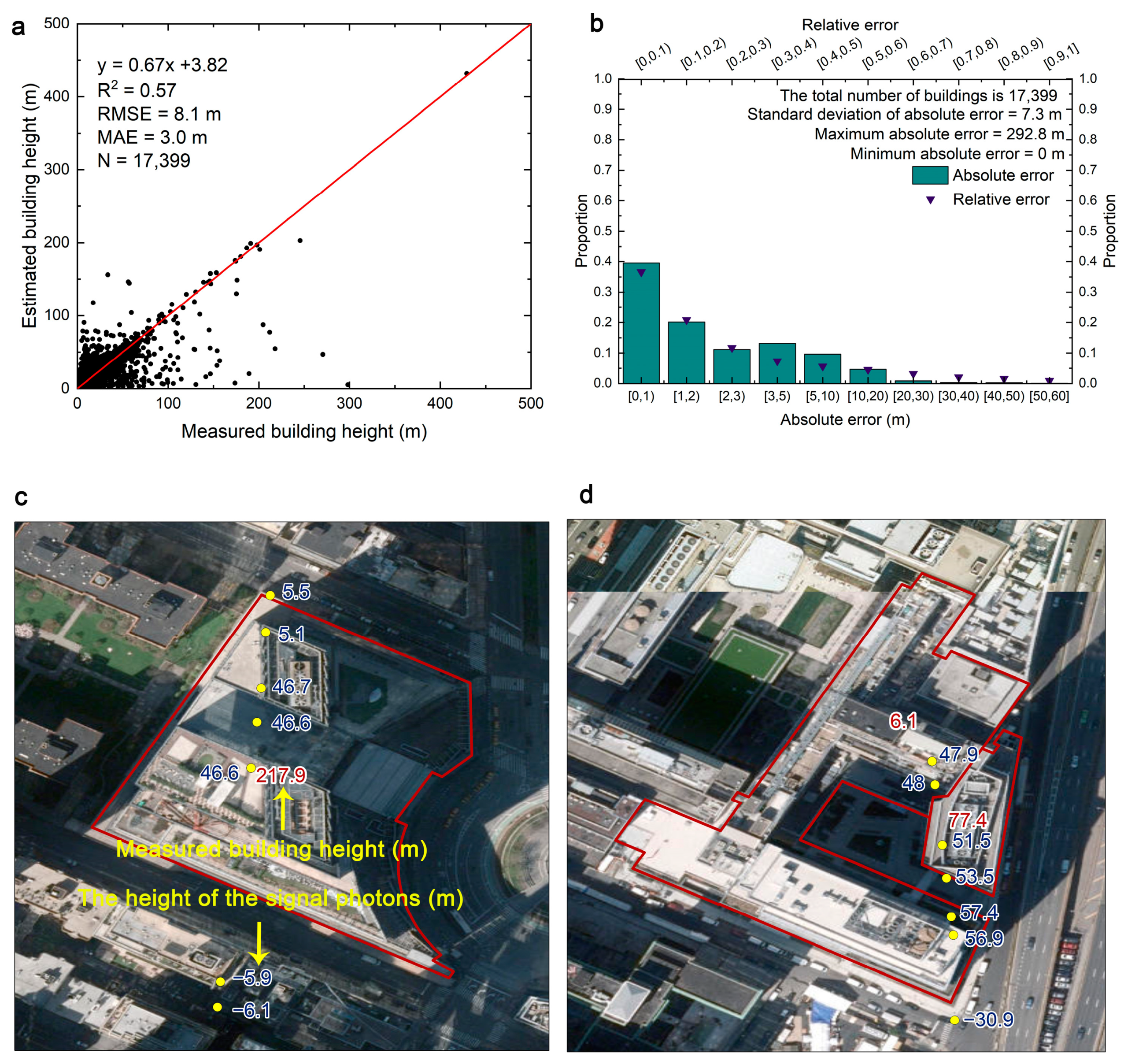
Good performance in New York City. The proposed method was successfully applied to estimate the heights of 17,399 buildings in New York City, achieving an RMSE of 8.1 m. Moreover, approximately 71% of the buildings exhibited an absolute difference of less than 3 m, demonstrating the effectiveness of our approach in a complex urban environment;

(3)

Strong robustness in varied conditions. The method demonstrated suitability for retrieving building heights under diverse conditions; its effectiveness can be extended to various geographical contexts.

However, it is important to acknowledge the limitations inherent in the discrete distribution of buildings obtained from ICESat-2 data. To overcome this limitation, future research should focus on merging multi-source data, such as optical images, SAR images, or digital surface model data, to obtain spatially continuous, large-scale, and high-precision building height datasets.

References

1. United Nations Environment Programme. Global Status Report for Buildings and Construction: Towards a Zero-Emission, Efficient and Resilient Buildings and Construction Sector; United Nations Environment Programme: Nairobi, Kenya, 2020. [Google Scholar]
2. Horowitz, C.A. Paris Agreement. Int. Leg. Mater. 2016, 55, 740–755. [Google Scholar] [CrossRef]
3. Borck, R. Will skyscrapers save the planet? Building height limits and urban greenhouse gas emissions. Reg. Sci. Urban. Econ. 2016, 58, 13–25. [Google Scholar] [CrossRef]
4. Glaeser, E.L.; Kahn, M.E. The greenness of cities: Carbon dioxide emissions and urban development. J. Urban. Econ. 2010, 67, 404–418. [Google Scholar] [CrossRef]
5. Li, M.; Koks, E.; Taubenböck, H.; van Vliet, J. Continental-scale mapping and analysis of 3D building structure. Remote Sens. Environ. 2020, 245, 111859. [Google Scholar] [CrossRef]
6. Kim, T.-Y.; Han, G.-S.; Kang, B.-S.; Lee, K.-H. Development of a risk assessment model against disasters in high-rise buildings and results of a building simulation analysis. J. Asian Arch. Build. Eng. 2022, 21, 249–262. [Google Scholar] [CrossRef]
7. Kumar, A. Review of building regulations for safety against hazards in Indian hill towns. J. Urban. Manag. 2018, 7, 97–110. [Google Scholar] [CrossRef]
8. Wu, T.; Perrings, C.; Kinzig, A.; Collins, J.; Minteer, B.; Daszak, P. Economic growth, urbanization, globalization, and the risks of emerging infectious diseases in China: A review. Ambio 2016, 46, 18–29. [Google Scholar] [CrossRef]
9. Du, Y.; Mak, C.M.; Tang, B.-S. Effects of building height and porosity on pedestrian level wind comfort in a high-density urban built environment. Build. Simul. 2018, 11, 1215–1228. [Google Scholar] [CrossRef]
10. Boo, G.; Darin, E.; Leasure, D.R.; Dooley, C.A.; Chamberlain, H.R.; Lázár, A.N.; Tschirhart, K.; Sinai, C.; Hoff, N.A.; Fuller, T.; et al. High-resolution population estimation using household survey data and building footprints. Nat. Commun. 2022, 13, 1330. [Google Scholar] [CrossRef]
11. Langford, M.; Higgs, G.; Radcliffe, J.; White, S. Urban population distribution models and service accessibility estimation. Comput. Environ. Urban. Syst. 2008, 32, 66–80. [Google Scholar] [CrossRef]
12. Alahmadi, M.; Atkinson, P.; Martin, D. Estimating the spatial distribution of the population of Riyadh, Saudi Arabia using remotely sensed built land cover and height data. Comput. Environ. Urban. Syst. 2013, 41, 167–176. [Google Scholar] [CrossRef]
13. Oke, T.R. City size and the urban heat island. Atmos. Environ. 1973, 7, 769–779. [Google Scholar] [CrossRef]
14. Khandelwal, S.; Goyal, R.; Kaul, N.; Mathew, A. Assessment of land surface temperature variation due to change in elevation of area surrounding Jaipur, India. Egypt. J. Remote Sens. Space Sci. 2018, 21, 87–94. [Google Scholar] [CrossRef]
15. Salvati, L.; Zitti, M.; Sateriano, A. Changes in city vertical profile as an indicator of sprawl: Evidence from a Mediterranean urban region. Habitat. Int. 2013, 38, 119–125. [Google Scholar] [CrossRef]
16. Goetz, M. Towards generating highly detailed 3D CityGML models from OpenStreetMap. Int. J. Geogr. Inf. Sci. 2013, 27, 845–865. [Google Scholar] [CrossRef]
17. OpenStreetMap. OpenStreetMap. Available online: https://www.openstreetmap.org/#map=5/38.007/-95.844 (accessed on 1 December 2023).
18. Biljecki, F.; Ledoux, H.; Stoter, J. Generating 3D city models without elevation data. Comput. Environ. Urban. Syst. 2017, 64, 1–18. [Google Scholar] [CrossRef]
19. Zhou, J.; Luo, C.; Jiang, W.; Yu, X.; Wang, P. Using UAVs and robotic total stations in determining height differences when crossing obstacles. Measurement 2022, 188, 110372. [Google Scholar] [CrossRef]
20. Abdulrahman, F.; Zaia, Y.; Gilyane, S. Height Evaluation and Linear Accuracy of Digital Level, Total station, GPS and Orthophoto. Acad. J. Nawroz Univ. 2018, 7, 27. [Google Scholar] [CrossRef]
21. Zhao, Y.; Wu, B.; Li, Q.; Yang, L.; Fan, H.; Wu, J.; Yu, B. Combining ICESat-2 photons and Google Earth Satellite images for building height extraction. Int. J. Appl. Earth Obs. Geoinf. 2023, 117, 103213. [Google Scholar] [CrossRef]
22. Park, Y.; Guldmann, J.-M. Creating 3D city models with building footprints and LIDAR point cloud classification: A machine learning approach. Comput. Environ. Urban. Syst. 2019, 75, 76–89. [Google Scholar] [CrossRef]
23. Sun, Y.; Mou, L.; Wang, Y.; Montazeri, S.; Zhu, X.X. Large-scale building height retrieval from single SAR imagery based on bounding box regression networks. ISPRS J. Photogramm. Remote Sens. 2022, 184, 79–95. [Google Scholar] [CrossRef]
24. Frantz, D.; Schug, F.; Okujeni, A.; Navacchi, C.; Wagner, W.; van der Linden, S.; Hostert, P. National-scale mapping of building height using Sentinel-1 and Sentinel-2 time series. Remote Sens. Environ. 2021, 252, 112–128. [Google Scholar] [CrossRef]
25. Brunner, D.; Lemoine, G.; Bruzzone, L.; Greidanus, H. Building Height Retrieval From VHR SAR Imagery Based on an Iterative Simulation and Matching Technique. IEEE Trans. Geosci. Remote Sens. 2010, 48, 1487–1504. [Google Scholar] [CrossRef]
26. Li, X.; Zhou, Y.; Gong, P.; Seto, K.C.; Clinton, N. Developing a method to estimate building height from Sentinel-1 data. Remote Sens. Environ. 2020, 240, 111705. [Google Scholar] [CrossRef]
27. Cao, Y.; Huang, X. A deep learning method for building height estimation using high-resolution multi-view imagery over urban areas: A case study of 42 Chinese cities. Remote Sens. Environ. 2021, 264, 112590. [Google Scholar] [CrossRef]
28. Yang, C.; Zhao, S. A building height dataset across China in 2017 estimated by the spatially-informed approach. Sci. Data 2022, 9, 76. [Google Scholar] [CrossRef]
29. Huang, H.; Chen, P.; Xu, X.; Liu, C.; Wang, J.; Liu, C.; Clinton, N.; Gong, P. Estimating building height in China from ALOS AW3D30. ISPRS J. Photogramm. Remote Sens. 2022, 185, 146–157. [Google Scholar] [CrossRef]
30. Misra, P.; Avtar, R.; Takeuchi, W. Comparison of Digital Building Height Models Extracted from AW3D, TanDEM-X, ASTER, and SRTM Digital Surface Models over Yangon City. Remote Sens. 2018, 10, 2008. [Google Scholar] [CrossRef]
31. Bonczak, B.; Kontokosta, C.E. Large-scale parameterization of 3D building morphology in complex urban landscapes using aerial LiDAR and city administrative data. Comput. Environ. Urban. Syst. 2019, 73, 126–142. [Google Scholar] [CrossRef]
32. Cheng, F.; Wang, C.; Wang, J.; Tang, F.; Xi, X. Trend analysis of building height and total floor space in Beijing, China using ICESat/GLAS data. Int. J. Remote Sens. 2011, 32, 8823–8835. [Google Scholar] [CrossRef]
33. Yang, X.; Wang, C.; Xi, X.; Wang, P.; Lei, Z.; Ma, W.; Nie, S. Extraction of Multiple Building Heights Using ICESat/GLAS Full-Waveform Data Assisted by Optical Imagery. IEEE Geosci. Remote Sens. Lett. 2019, 16, 1914–1918. [Google Scholar] [CrossRef]
34. Seidleck, M. The ice, cloud, and land elevation satellite-2—Overview, science, and applications. In Proceedings of the 2018 IEEE Aerospace Conference, Big Sky, MT, USA, 3–10 March 2018; pp. 1–8. [Google Scholar]
35. Lao, J.; Wang, C.; Zhu, X.; Xi, X.; Nie, S.; Wang, J.; Cheng, F.; Zhou, G. Retrieving building height in urban areas using ICESat-2 photon-counting LiDAR data. Int. J. Appl. Earth Obs. Geoinf. 2021, 104, 102596. [Google Scholar] [CrossRef]
36. Han, L.; Li, L.; Chen, H. Evaluation of the Significant Wave Height from HY2B/ALT Using Cryosat2/SIRAL and ICESAT2/ATLAS Data Sets in the Arctic. In Proceedings of the International Geoscience and Remote Sensing Symposium (IGARSS), Brussels, Belgium, 11–16 July 2021; pp. 7572–7575. [Google Scholar]
37. Ma, X.; Zheng, G.; Chi, X.; Yang, L.; Geng, Q.; Li, J.; Qiao, Y. Mapping fine-scale building heights in urban agglomeration with spaceborne lidar. Remote Sens. Environ. 2023, 285, 113392. [Google Scholar] [CrossRef]
38. Liu, A.; Cheng, X.; Chen, Z. Performance evaluation of GEDI and ICESat-2 laser altimeter data for terrain and canopy height retrievals. Remote Sens. Environ. 2021, 264, 112571. [Google Scholar] [CrossRef]
39. Xie, J.; Huang, G.; Liu, R.; Zhao, C.; Dai, J.; Jin, T.; Mo, F.; Zhen, Y.; Xi, S.; Tang, H.; et al. Design and Data Processing of China’s First Spaceborne Laser Altimeter System for Earth Observation: GaoFen-7. IEEE J. Sel. Top. Appl. Earth Obs. Remote Sens. 2020, 13, 1034–1044. [Google Scholar] [CrossRef]
40. Dandabathula, G.; Sitiraju, S.R.; Jha, C.S. Retrieval of building heights from ICESat-2 photon data and evaluation with field measurements. Environ. Res. Inf. Sustain. 2021, 1, 011003. [Google Scholar] [CrossRef]
41. Goud, G.P.S.; Bhardwaj, A. Estimation of Building Heights and DEM Accuracy Assessment Using ICESat-2 Data Products. Eng. Proc. 2021, 10, 37. [Google Scholar] [CrossRef]
42. U.S. Census Bureau. Measuring America’s People, Places, and Economy. Available online: https://www.census.gov/quickfacts/fact/table/newyorkcitynewyork,bostoncitymassachusetts,US/LND110210 (accessed on 1 December 2023).
43. Statista Research Department. Real Gross Domestic Product of New York in the United States from 2000 to 2022. Available online: https://www.statista.com/statistics/188087/gdp-of-the-us-federal-state-of-new-york-since-1997/#statisticContainer (accessed on 1 December 2023).
44. Neumann, T.A.; Martino, A.J.; Markus, T.; Bae, S.; Bock, M.R.; Brenner, A.C.; Brunt, K.M.; Cavanaugh, J.; Fernandes, S.T.; Hancock, D.W.; et al. The Ice, Cloud, and Land Elevation Satellite—2 mission: A global geolocated photon product derived from the Advanced Topographic Laser Altimeter System. Remote Sens. Environ. 2019, 233, 111325. [Google Scholar] [CrossRef]
45. Hawker, L.; Uhe, P.; Paulo, L.; Sosa, J.; Savage, J.; Sampson, C.; Neal, J. A 30 m global map of elevation with forests and buildings removed. Environ. Res. Lett. 2022, 17, 024016. [Google Scholar] [CrossRef]
46. Karra, K.; Kontgis, C.; Statman-Weil, Z.; Mazzariello, J.C.; Mathis, M.; Brumby, S.P. Global land use/land cover with Sentinel 2 and deep learning. In Proceedings of the 2021 IEEE International Geoscience and Remote Sensing Symposium IGARSS, Brussels, Belgium, 11–16 July 2021; pp. 4704–4707. [Google Scholar]
47. Neumann, T.A.; Brenner, A.; Hancock, D.; Robbins, J.; Saba, J.; Harbeck, K.; Gibbons, A.; Lee, J.; Luthcke, S.B.; Rebold, T. ATLAS/ICESat-2 L2A Global Geolocated Photon Data, Version 5; NASA National Snow and Ice Data Center Distributed Active Archive Center: Boulder, CO, USA, 2021. [Google Scholar] [CrossRef]
48. Wu, B.; Huang, H.; Zhao, Y. Utilizing Building Offset and Shadow to Retrieve Urban Building Heights with ICESat-2 Photons. Remote Sens. 2023, 15, 3786. [Google Scholar] [CrossRef]
Figure 1. Map of New York City showing a portion of the ICESat-2 ground tracks. The yellow lines indicate the satellite’s path and represent the photon-counting events collected by the ATLAS instrument (Chambersburg, PA, USA).
Remotesensing 16 00263 g001
Figure 2. The flowchart of building height estimation.
Remotesensing 16 00263 g002
Figure 3. Challenges in extracting building heights using ICESat-2/ATL03 with the aid of building footprints. (ae) highlight problems i–v, and Figure (f) is a legend. Height is measured in meters.
Remotesensing 16 00263 g003
Figure 4. Selection of building photons. In (a), represents a square building, (b) represents an irregular building, (c) portrays a building with an open space in the center, and (d) showcases a multi-story building with varying sizes.
Remotesensing 16 00263 g004
Figure 5. Accuracy of building height estimation. In (a), a scatter plot compares the measured building height of BuildingFootprints NYC with the estimated building height from ATL03. (b) displays the frequency distribution of the absolute difference and relative error between the measured and estimated building heights. Additionally, (c,d) highlight the main instances of outliers observed in (a). Within the figure, the red polygons depict building footprints, while the yellow dots represent photons. The red numbers indicate the height of the building footprint markers, whereas the blue numbers indicate the height of the photon markers, measured in meters.
Remotesensing 16 00263 g005
Figure 6. Accuracy under different parameter settings. Figure (a,b) demonstrate that the threshold d remain unchanged, while the R2 and RMSE vary with the variable thresholds m and h. On the other hand, Figure (c) illustrates that the thresholds m and h remain constant, and the precision RMSE changes with the variable threshold d.
Remotesensing 16 00263 g006
Figure 7. Scatter plot of estimated versus measured building heights before and after abnormal terrain fluctuations were removed. (a) before terrain filtering, (b) after terrain filtering.
Remotesensing 16 00263 g007
Figure 8. Accuracy and number of the estimated building height under different distance thresholds. The distance is represented by the portion of the minimum width of the building footprint between the photons and the geometric center of the building.
Remotesensing 16 00263 g008
Figure 9. Accuracy and number of the estimated building height under different environments. (a) under different slopes, (b) under different Boroughs, (c) under different building heights, (d) under different building densities.
Remotesensing 16 00263 g009
Figure 10. The complexity of buildings and the accuracy of building height estimation. Figure (ad) depict the comparison between the estimated and measured building heights for different levels of complexity in building structures. Within the figure, the red polygons depict building footprints, while the yellow dots represent photons. The red numbers indicate the height of the building footprint markers, whereas the black numbers indicate the height of the photon markers, measured in meters.
Remotesensing 16 00263 g010