Article

Scene Classification Method Based on Multi-Scale Convolutional Neural Network with Long Short-Term Memory and Whale Optimization Algorithm

1
College of Mechanical and Electrical Engineering, Hohai University, Changzhou 213022, China
2
Jiangsu Key Laboratory of Special Robot Technology, Hohai University, Changzhou 213022, China
3
College of Mechanical Engineering, Yangzhou University, Yangzhou 225127, China
*
Author to whom correspondence should be addressed.
Remote Sens. 2024, 16(1), 174; https://doi.org/10.3390/rs16010174
Submission received: 29 October 2023 / Revised: 26 December 2023 / Accepted: 29 December 2023 / Published: 31 December 2023
(This article belongs to the Special Issue Advances in the Application of Lidar)

Abstract

:
Indoor mobile robots can be localized by using scene classification methods. Recently, two-dimensional (2D) LiDAR has achieved good results in semantic classification with target categories such as room and corridor. However, it is difficult to achieve the classification of different rooms owing to the lack of feature extraction methods in complex environments. To address this issue, a scene classification method based on a multi-scale convolutional neural network (CNN) with long short-term memory (LSTM) and a whale optimization algorithm (WOA) is proposed. Firstly, the distance data obtained from the original LiDAR are converted into a data sequence. Secondly, a scene classification method integrating multi-scale CNN and LSTM is constructed. Finally, WOA is used to tune critical training parameters and optimize network performance. The actual scene data containing eight rooms are collected to conduct ablation experiments, highlighting the performance with the proposed algorithm with 98.87% classification accuracy. Furthermore, experiments with the FR079 public dataset are conducted to demonstrate that compared with advanced algorithms, the classification accuracy of the proposed algorithm achieves the highest of 94.35%. The proposed method can provide technical support for the precise positioning of robots.

1. Introduction

With the development of artificial intelligence, robots have evolved to possess comprehensive functionalities, expanded applications and adaptability to complex environments. Robots are utilized in industries, agriculture, household tasks and other fields. In terms of mobility, robots can be categorized into two main types: fixed robots and mobile robots. A fixed robot is typically mounted on a stationary base and its movement depends on joints. On the other hand, a mobile robot can navigate in unrestricted directions, and its ability of real-time locating during task performance becomes imperative. Robot positioning techniques include relative methods based on odometry and inertial navigation, and absolute methods such as navigation beacons, graphic matching, global scene features, Global Positioning System (GPS) and probabilistic positioning.
Based on the sensor type utilized, scene classification methods are typically categorized into two types: visual-based methods and laser-based methods. Visual-based methods generally use deep learning for scene recognition through object detection and the construction of semantic maps. With the development of target detection and semantic segmentation methods such as Region with Convolutional Neural Network (R-CNN), Fast R-CNN, Faster R-CNN, You Only Look Once (YOLO) and Single Shot MultiBox Detector (SSD) [1,2,3,4,5], visual-based methods have made significant progress. Sünderhauf proposed the integration of an SSD target detection method and unsupervised three-dimensional (3D) segmentation algorithm and applied it in RGB-D Simultaneous Localization and Mapping (SLAM) [6], establishing an instance-level, object-oriented semantic octree map [7]. Sharma proposed a novel SLAM [8]. By combining geometry-based techniques with object detection, indoor scenes were represented as graphs of objects. Other methods focus on direct scene classification. Ni proposed an improved Faster R-CNN and residual attention module to classify five outdoor scenes, and the accuracy could reach 94.76% [9]. Li achieved an accuracy of 56.2% on the SUN RGB-D dataset by using Multi Attending Path Neural Network (MAPNet) [10], surpassing Song’s algorithm [11]. Recently, Mosella-Montoro and Zhou used a graph convolution neural network for scene classification [12,13]. These methods primarily rely on local semantic cues. However, insensitive computation is required in the process of image recognition for these methods.
On the other hand, laser-based methods are constantly being studied. Since 3D laser LiDAR captures rich spatial information [14], 3D scene classification is often utilized. Chen proposed LiDAR-based Semantic SLAM, which adds semantic constraints to improve the robustness and accuracy of localization [15]. The semantic information in the scanned data is effectively extracted through neural network, and the tags are generated to obtain the semantic map. Compared with 3D LiDAR, 2D LiDAR is more frequently used in indoor scenes. Kosnar developed a shape-matching method based on 2D range data, suitable for position recognition in robot mapping environments [16]. Recently, machine learning has been employed in 2D laser scene classification. Mozos used the range data and extracted the features, such as the average and standard deviation of the beam length, to distinguish doorways, corridors and rooms with an AdaBoost algorithm [17]. Sousa recognized the rooms and corridors by using an SVM algorithm to recognize rooms and a single corridor, achieving an accuracy of 80% [18]. Park proposed a method of location classification using range scanning, and used 2D-PCA to extract features from a 2D diagonal distance histogram [19]. Kaleci proposed a probabilistic method based on laser distance, classifying indoor environments as rooms, corridors and doors. This method employs clustering of raw 2D laser measurements to distinguish structures, and uses K-means and LVQ methods to classify robot positions [20]. Shi presented an approach to classify the environment around a robot based on laser range and bearing. The perceived information together with a partial understanding of the geometric structure of the environment were then applied to accumulatively build a labeled semantic grid map [21]. Kaleci introduced a rule-based doorway detection algorithm which combines K-means clustering and template matching classification methods. It results in a semantic classification approach for indoor environments using 2D range information [22]. These methods accomplish detection by using designed features and range data, yet they lack the capability to extract features automatically.
As computational power continues to evolve, deep learning has become a valuable tool in the realm of classifying scenes using 2D laser. Kaleci proposed a point-based deep learning architecture called 2DLaserNet, which uses the ordered relationships between successive points in the point cloud generated from 2D laser readings to learn the geometric characteristics corresponding to the laser scans of rooms, corridors and doorways [23]. Yu used a convolutional neural network to solve the kidnapped robot problem. The laser data were converted into an RGB image and an occupancy grid map, which were then stacked into a multi-channel image. Moreover, the position information was added into the neural network input, and the convolutional neural network model was designed to regress the robot attitude [24]. Goeddel demonstrated the effectiveness of CNN in learning semantic place labels from 2D range data [25]. By increasing the diversity of training data, CNN can be applied to different environments. Nikdel presented a system to describe the navigational cues around a robot using a combination of 2D LiDAR data and occupancy grid maps. The CNN was trained to predict the closed rooms, open rooms and intersections around the robot. A tracking module aggregated the predictions to locate and classify the navigational cues with enhanced accuracy [26]. Zheng proposed a novel approach to obtain semantic labels of 2D LiDAR room maps by combining the distance transform watershed-based pre-segmentation and a skillfully designed fast and efficient neural network LiDAR information sampling classification [27]. Turgut and Kaleci used MLP to semantically classify different rooms, corridors and doors [28]. Liao proposed an end-to-end learning approach for place classification [29]. With the deep architecture, features were found automatically and classification accuracy was improved.
In summary, current research on the scene classification of robots primarily emphasizes multi-dimensional data. However, in practical applications, indoor robots commonly employ cost-effective sensors such as cameras and 2D LiDAR. Since visual-based methods require intensive calculations and are susceptible to lighting conditions and viewing angles, their applicable scenarios are constrained. On the contrary, 2D LiDAR offers reliable data at a relatively low cost, making it a favored choice for indoor robots. Although there are numerous reports on the classification of rooms and corridors based on 2D LiDAR, they primarily focus on the classification between categories rather than distinguishing between rooms. Therefore, this paper introduces a global scene feature localization method based on 2D LiDAR and CNN for scene classification. Without providing the precise coordinates of the robot position [30], this method classifies the scene itself where the robot is located.
Our contributions are as follows:
(1)
This paper proposes a network capable of indoor scene recognition using 2D LiDAR. It is composed of a multi-scale CNN and LSTM network, which can effectively classify distance features and resolve the long-term dependence issue of neural networks.
(2)
A WOA algorithm is used to automatically optimize the initial learning rate, the regularization parameters and the parameters of the LSTM hidden layer of the neural network. The algorithm significantly reduces the time spent on manual parameter tuning, and achieves promising results in scene classification.
The rest of this paper is organized as follows: Section 2 introduces the network structure of the proposed method. Section 3 introduces the datasets and describes the evaluation indexes, followed by ablation experiments and a performance comparison with other methods. Section 4 summarizes the conclusions.

2. Scene Recognition Method Based on CNN for 2D LiDAR

2.1. LiDAR Data Preprocessing

The 2D LiDAR rotates 360 degrees to acquire a single frame of laser data, capturing information of the surrounding environment. Figure 1 illustrates LiDAR angle range with a field of view of 270 degrees. Point clouds are represented using polar coordinates, consisting of range and angle information. Depending on the environmental characteristics, these laser point clouds exhibit different arrangements. In this paper, we transform the range ρ and the corresponding serial number in polar coordinates into Cartesian coordinates, thus converting the laser data into a data sequence of distance information with serial numbers.
Figure 2a,b are the laser data of the 1st and 150th frames of Room 1, while Figure 3a,b are the corresponding laser data of Room 2. It is evident that the laser data between different frames in the same room are similar, while the difference in laser data between different rooms is significant. Therefore, after collecting sufficient laser data, the deep learning method is employed to extract different features for room classification.

2.2. Network with CNN and LTSM

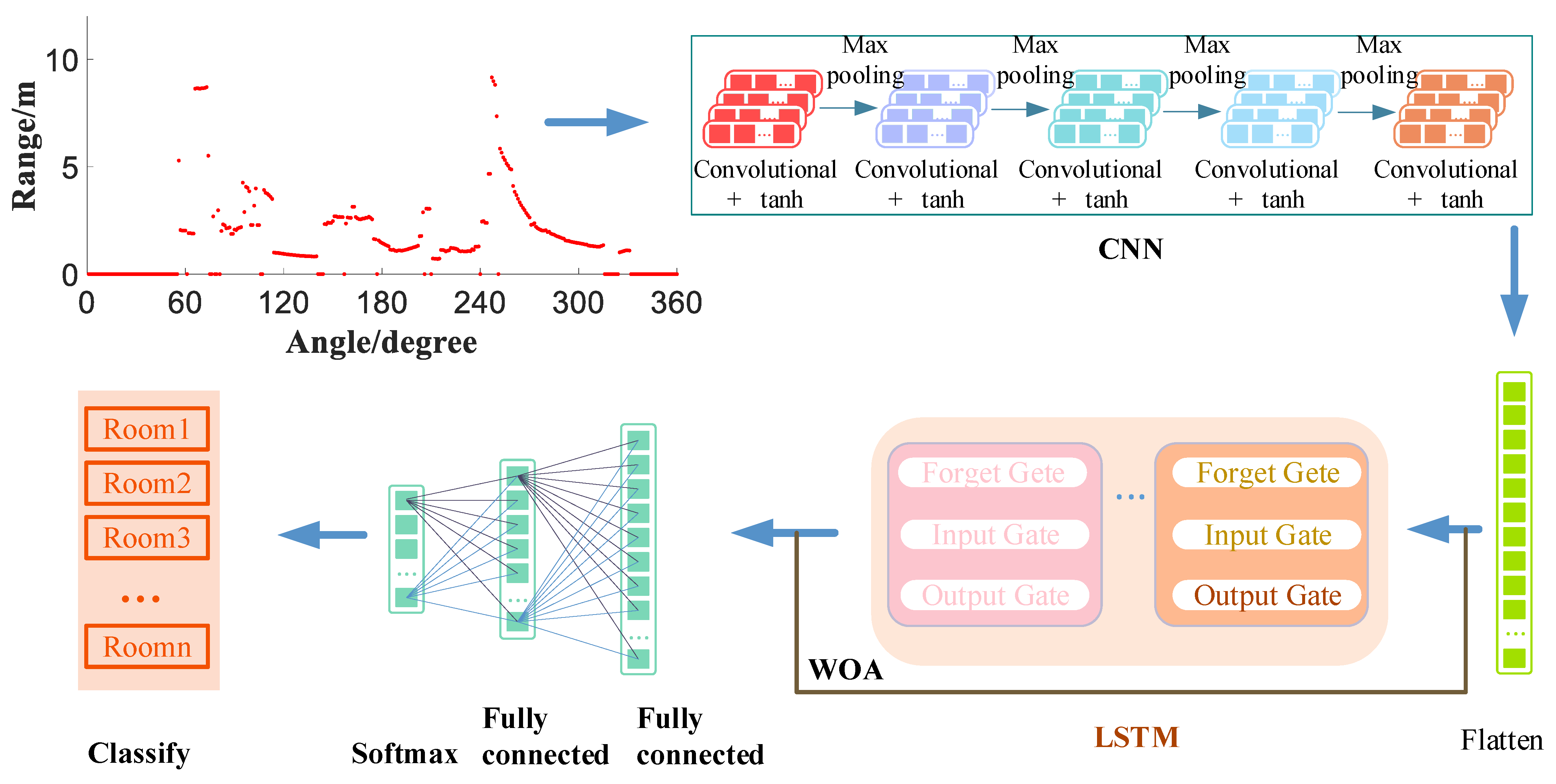
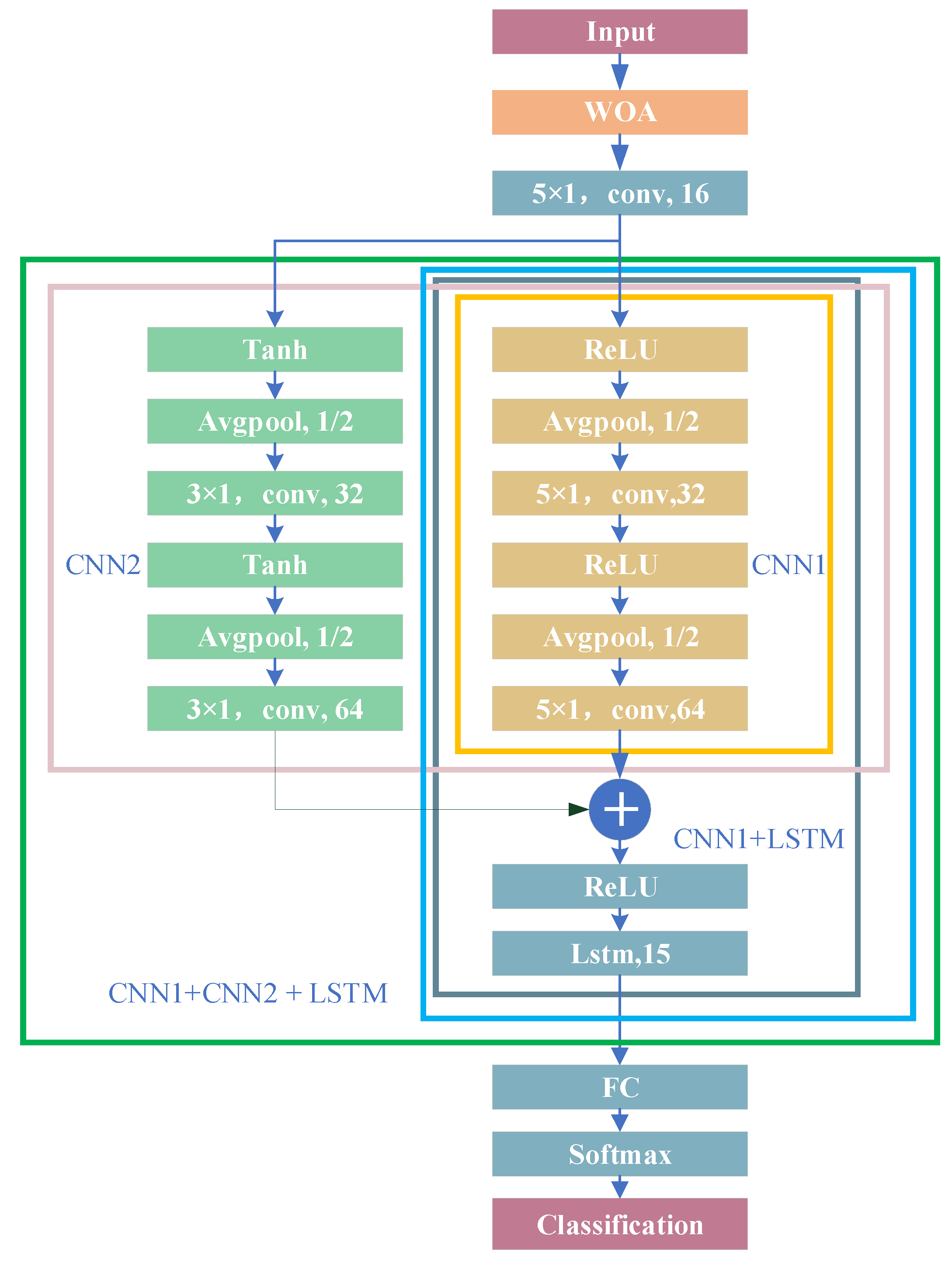
In this paper, a network integrating CNN and LSTM is proposed. CNN only captures spatial information and LSTM further extracts the implicit spatial–temporal features from the time series data. The algorithm flowchart is shown in Figure 4. Firstly, features of the laser data of different rooms are extracted by CNN. Then, multiple features extracted by CNN are flattened and fed into the LSTM network. Finally, the full connection and softmax are used for room recognition.
To optimize the network, manual parameter tuning is necessary but time-consuming. Therefore, a WOA intelligent optimization algorithm is employed for autonomous searching of the optimal value.

2.2.1. Multi-Scale CNN Network

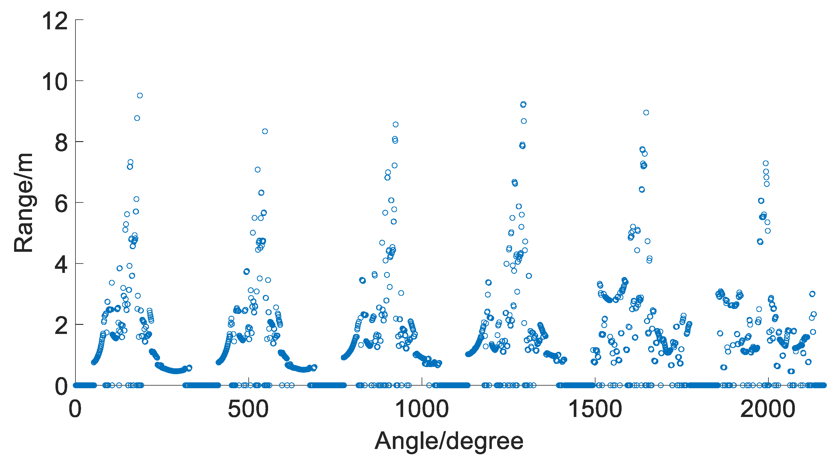
A single frame of laser data depends on the minimum angle resolution of LiDAR. The angular resolution of the Slamtec rplidar A2 LiDAR employed is 0.225 degrees. The minimum size of the obstacle is proportional to the distance from the obstacle. For instance, considering a distance of 5 m to the obstacle, the minimum detectable size of the obstacle is 1.96 cm. To reduce the amount of calculation, data compression is performed. Direct data association exists between the front and back frames of the laser. Several frames of data in Room 4 are extracted for interception and splicing, as depicted in Figure 5. It is evident that there are variations in the laser distributions collected by robots in different locations. Their features can be extracted by CNN.
Some CNN networks have demonstrated outstanding performances in recognition tasks. For example, LeNet5, a handwritten font recognition model, is one of the earliest classic CNN networks [31]. Alexnet is the first large-scale CNN network that performs well in ImageNet classification [32]. Inception V1 (GoogleNet) is a deep neural network model based on the Inception module launched by Google, which increases the network depth and width [33]. Visual Geometry Group (VGG) has excellent performance in multiple transfer learning tasks [34]. Residual Neural Network (ResNet), which breaks network depth constraints, is a classic neural network for visual classification [35].
In this paper, a multi-scale CNN network is proposed to improve the accuracy of scene feature extraction. The dual-scale CNN framework is illustrated in Figure 6. It can extract detailed features of different scales and obtain a larger receptive field, allowing more valuable information to be preserved.

2.2.2. LSTM Algorithm

Although the multi-scale CNN can extract the spatial features, it tends to overlook the temporal ones. Therefore, the LSTM network is employed [36]. LSTM is a temporal recurrent network, which is used to solve the long-term dependence problem of neural networks. The synergy of multi-scale CNN with LSTM enhances the network’s overall accuracy.
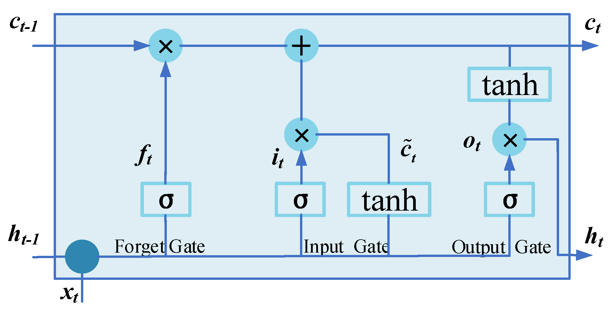
The internal structure of LSTM is illustrated in Figure 7. The network comprises three inputs and two outputs. xt represents the input value of the network at the current time, ct−1 denotes the cell state at the previous time and ht−1 is the output value of the LSTM network at the previous time. ct is the cell state at the current time, and ht is the output value of the LSTM network at the current time.
The control unit consists of three gates: the forget gate, the input gate and the output gate. The forget gate ft determines whether ct−1 can be retained to ct. The input gate it determines whether xt can be input into ct, where c ˜ t , as a temporary cell state unit, controls the cell unit updates. The output gate ot controls whether ct is passed to ht.
The expressions for the forget gate, the input gate and the output gate are as follows:
f t = σ ( W f x t + U f h t 1 + b f )
i t = σ ( W i x t + U i h t 1 + b i )
c ˜ t = tanh ( W c x t + U c h t 1 + b c )
o t = σ ( W o x t + U o h t 1 + b o )
where Wf, Wi and Wo represent the weight vectors from the input layer to the input gate, the forget gate and the output gate, respectively. Uf, Ui and Uo represent the weight vector from the hidden layer to the input gate, the forget gate and the output gate, respectively. bf, bi and bo represent bias vectors from the input layer to the input gate, forget gate and output gate, respectively. σ(.) refers to the sigmoid activation function, and tanh refers to the hyperbolic tangent activation function, representing the multiplication of vector elements.
In order to calculate the predicted value yt and generate the complete input for the next time slice, we need to calculate the output ht of the hidden node. ht is obtained from the output gate ot and unit state ct, where ot is calculated in the same way as ft and it. In conventional applications, the final predicted value Pt is obtained from ht through full connection.
c t = f t c t 1 + i t c ˜ t
i t = σ ( W i x t + U i h t 1 + b i )
LSTM regulates the transmission of historical information through gate functions and possesses capabilities in processing and predicting time series data. In theory, a longer stride in CNN can extract more information. However, when the stride becomes excessively long, long-distance memory loss and gradient vanishing may occur. By combining CNN and LSTM, it is possible to effectively extract sequence features and preserve extended and valuable memory information, thereby addressing the issue of gradient vanishing.

2.2.3. WOA Algorithm

Parameter tuning of deep learning is time-consuming, and the use of intelligent optimization algorithms can address this issue through autonomous learning. Due to the attributes of a fast rate of convergence, robust global search ability and ease of implementation [37], WOA is selected in this paper to automatically search for optimal parameters.
WOA optimizes the search process by simulating humpback whale hunting behavior, including searching, surrounding and pursuing prey. The initial position of the whale is
X = ( x 1 , x 2 , , x n )
The position of each whale represents a feasible solution, and WOA progressively converges towards the optimal solution by continuously searching and updating their positions. The WOA algorithm includes three mathematical models: encircling prey, bubble hunting and searching prey. In the process of encircling prey, since the algorithm cannot yet identify the optimal position, the WOA algorithm assumes that the current best candidate position is the target prey position. The whale group encircles the prey from this assumed position, and continuously updates to explore various positions around the optimal solution.
D = | C X * ( t ) X ( t ) |
X ( t + 1 ) = X * ( t ) A D
where t represents the current iteration, A and C are coefficient vectors, X * is the position vector of the best solution obtained thus far, X is the position vector, | | denotes the absolute value and represents element-by-element multiplication. It is worth mentioning that X * should be updated during each iteration if a better solution exists.
The vectors A and C are calculated as follows:
A = 2 a r a
C = 2 r
where a iterates throughout the exploration and development phase, linearly decreasing from 2 to 0, and r is a random vector in [0, 1].
Shrinking encircling mechanism: This behavior is achieved by decreasing the value of a . Note that the fluctuation range of A is also narrowed as a decreases. In other words, A is a random value in the interval of [−a, a], where a decreases from 2 to 0 over the course of iterations. By setting a random value for A in the range of [−1, 1], the new position of a search agent whale can be defined anywhere between the original position of the agent and the position of the current best agent.
Spiral updating position: The distance between the whale’s coordinates (X, Y) and the prey’s coordinates (X*, Y*) is calculated. Then, a spiral equation is constructed between the whale and the prey to mimic the spiral motion of a humpback whale as follows:
X ( t + 1 ) = D e b l cos ( 2 π l ) + X * ( t )
D = | X * ( t ) X ( t ) |
where D is the distance between the ith whale and the prey, b is a constant defining the logarithmic spiral shape and l is a random number in the range of [−1, 1].
In the prey search phase, whales randomly select the location of a single whale as a reference to update their next locations, and search for the next prey globally.
In the exploration phase, the method based on A vector variation is also used to search for prey. Because humpback whales search randomly based on their positions relative to each other, a random value A can be used with an absolute value greater than 1 to force the search agent to diverge from a reference whale. In contrast to the development phase, the location of the search agent is updated based on a randomly selected search agent. The mathematical model is expressed as follows:
D = | C X r a n d X |
X ( t + 1 ) = X r a n d A D
where X r a n d is a random position vector (a random whale) chosen from the current population.
Using the WOA algorithm to train the initial learning rate, the regularization parameters and the number of LSTMs enable autonomous parameter learning, resulting in an enhanced classification accuracy.

3. Results

This article validated the algorithm using data collected from the experiment and public datasets. Firstly, 2D laser data from multiple rooms were collected using a self-developed robot mobile platform. The algorithm proposed is used for room classification, and the effectiveness of the algorithm is verified through metrics including accuracy and recall. Secondly, to demonstrate the superiority of the proposed algorithm, a comparative assessment of the classification performance with other algorithms is conducted using a public dataset.

3.1. Results on Laboratory Datasets

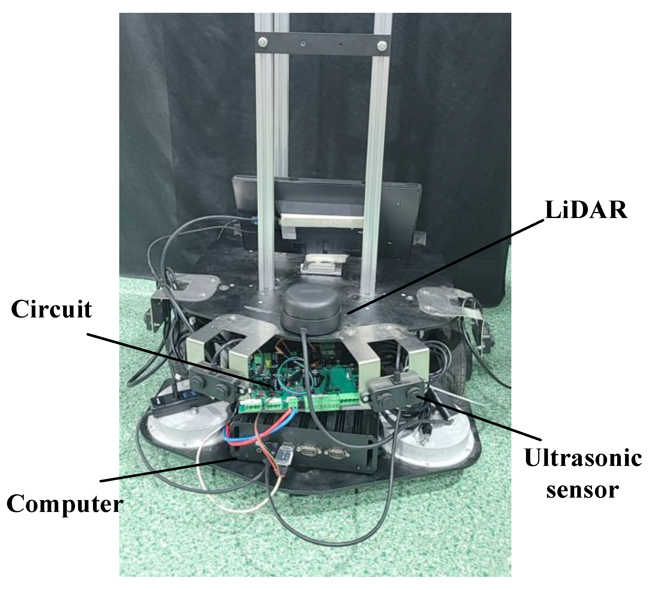
The self-developed indoor mobile robot experimental platform is depicted in Figure 8. It is equipped with a 2D LiDAR (RPLIDAR A2), six ultrasonic sensors and an IMU, capable of mapping and autonomous navigation.
The mobile robot platform was used to collect the data of eight rooms on the first floor of Yingcai building in Changzhou Campus of Hohai University. The distribution of obstacles in the laboratory were irregular. Figure 9 shows the 80th frames of the 2D LiDAR data in Rooms 1 to 8, revealing distinct contour profiles for each room. Corresponding room mappings generated using cartographer are displayed in Figure 10 for reference. The dataset collected by the robot contains a total of 8256 frames, including 2300, 1965, 590, 431, 526, 443, 1026 and 975 frames of Rooms 1 to 8, respectively.
In the above dataset, 70% of the frames were randomly selected as the training set, while 20% were designated as the validation set and the remaining 10% were allocated as the test set. The experiments were conducted on a computer running matlab2022, with a configuration of i7-10875H CPU and 16 GB Random Access Memory (RAM).

3.1.1. Evaluation Indexes

As shown in Figure 11, four networks were constructed to classify the eight rooms. Network 1 merely employs CNN1, Network 2 integrates both CNN1 and CNN2, Network 3 utilizes CNN1 in conjunction with LSTM and Network 4 incorporates CNN1, CNN2, and LSTM. It is worth noting that since the outputs of the CNN1 and CNN2 networks are directly added together, it is necessary to ensure that the size of output data is consistent, that is, edge supplement is required during the convolution process.
Accuracy, precision, F1 and recall are used for the evaluation. The parameters used from the confusion matrix include True Positive (TP), False Negative (FN), False Positive (FP) and True Negative (TN).
Accuracy refers to the proportion of correct predictions in the total sample, expressed as follows:
A c c u r a c y = T P + T N T P + T N + F P + T N
Precision is a measure of result reliability, indicated by how many positive samples are correct in the predicted results:
P r e c i s i o n = T P T P + F P
Recall is a measure of the number of genuinely relevant results returned, indicated by how many positive samples are correctly detected in the predicted results.
R e c a l l = T P T P + F N
F1 comprehensively considers the two indicators of precision and recall:
F 1 = 2 × P r e c i s i o n × R e c a l l P r e c i s i o n + R e c a l l
In multi-classification, the F1 values of all categories are calculated, and their average is called Macro-F1:
M a c r o F 1 = 1 n ( F 1 ) n n

3.1.2. Ablation Experiments

Ablation experiments were conducted to assess the performances of the networks with different combinations of CNNs and LSTM. Networks with each combination were trained five times, and the average of the five networks for each combination is displayed in Table 1. The accuracies of the four algorithms are listed in Table 1. The test results show that the classification accuracy of a single CNN network is 92.44%. Compared with a single CNN network, due to the different feature extraction capabilities provided by different CNN networks, the accuracy of the multi-scale CNN network with CNN1 and CNN2 is improved to 95.56%. Owing to the advantages of LSTM in global feature extraction, the combination of CNN and LSTM yields an even better result of a 5.86% increase in accuracy, which captures sequence features and filters out invalid features. By integrating multi-scale CNN with LSTM, the classification accuracy achieved is 98.91% due to the collaborative synergy between these two algorithms.
Ttotal represents the total training, validation and prediction time of the network, and Tprediction represents the prediction time of a single frame. As shown in Table 1, both Ttotal and the Tprediction show an increasing trend with CNN1, CNN1 + LSTM, CNN1 + CNN2 and CNN1 + CNN2 + LSTM, and the addition of CNN2 increased more time. However, in terms of accuracy, the improvement brought about by LSTM surpasses that of CNN2, emphasizing the crucial role of LSTM in the network. In addition, for the real-time performance of the robot, the CNN1 + CNN2 + LSTM network with the highest classification accuracy has a Ttotal of 152.40 s and a Tprediction of 0.1236 ms, which can fulfill the requirements of the robot.
As shown in Figure 12a,b, the recall, accuracy and precision of the model increase as the network incorporates more modules. In order to comprehensively evaluate the precision and recall, an F1 curve was used. As shown in Figure 12c, the F1 curve also demonstrates a similar synergistic effect of multiple modules, where the network CNN1 + CNN2 + LSTM exhibits evident advantages. The minimum value of F1 is 0.9647 and the maximum is 0.9975, which proves the effectiveness of the network in accurately identifying rooms. As shown in Table 1 and Figure 12d, the Macro-F1 is also benefited by the combined synergy of the three modules.
The recognition result of Room 6 is the best due to its distinctive characteristics compared to the other rooms. Considering the overall classification results of the eight rooms, it is evident that the proposed network possesses a notable classification capability.

3.1.3. Experiments of WOA Algorithm

To enhance the classification effectiveness, the combination of multi-scale CNN and LSTM is selected. However, during the network training, the initial learning rate, regularization coefficient and the number of LSTM networks require continuous optimization. To diminish manual debugging tasks, this paper adopts the WOA algorithm for autonomous tuning of these three types of parameters.
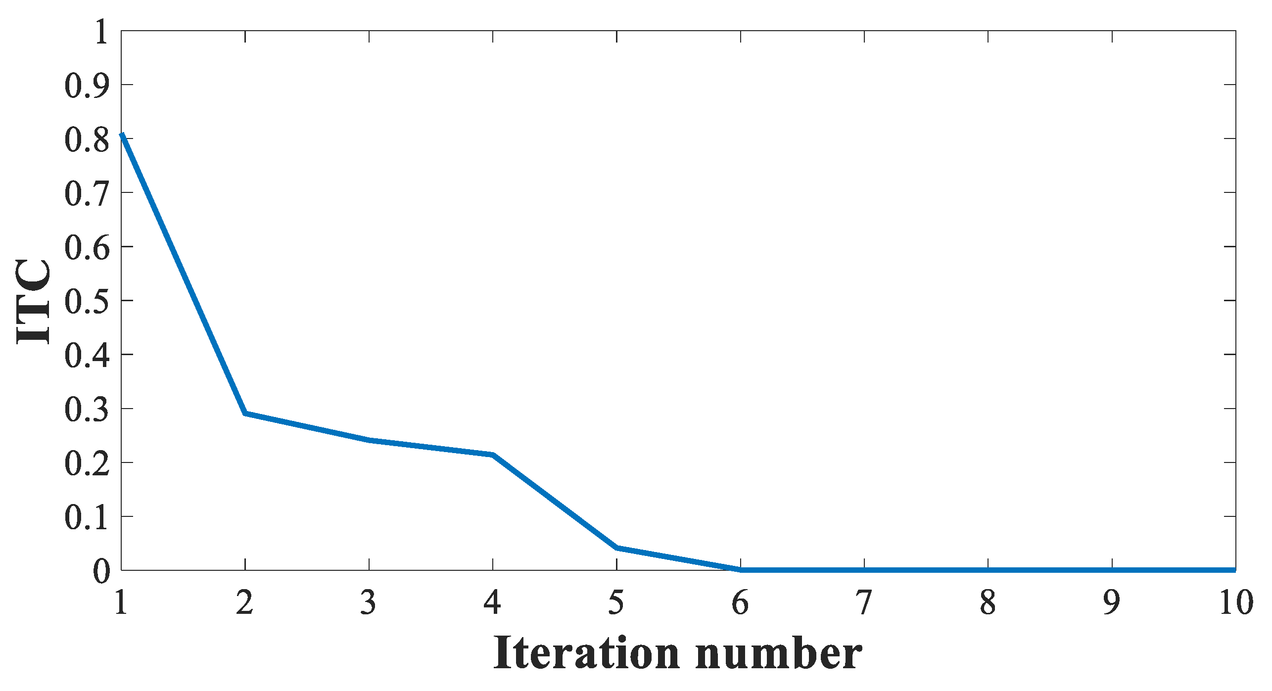
WOA optimization is a process that gradually approaches the optimal position through autonomous learning and tuning. The evaluation index of iterative training accuracy (ITC) reflects accuracy variations within each iteration during the training, thereby representing the optimization effectiveness of WOA. The ITC formula is as follows:
I T C i = 1 - ( A c c u r a c y t r a i n ) i
where i is the iteration number, and Accuracytrain is the training accuracy achieved in each iteration. The formula indicates the disparity between the results of each iteration and the optimal position.
The relationship between ITC and iteration number for the WOA algorithm is depicted in Figure 13. The WOA algorithm progressively approaches the optimal solution by iteratively updating the initial learning rate, the regularization coefficient and the number of LSTM networks, and the accuracy of the training set of this algorithm reaches 100% after three iterations, meaning the optimal solution has been attained.
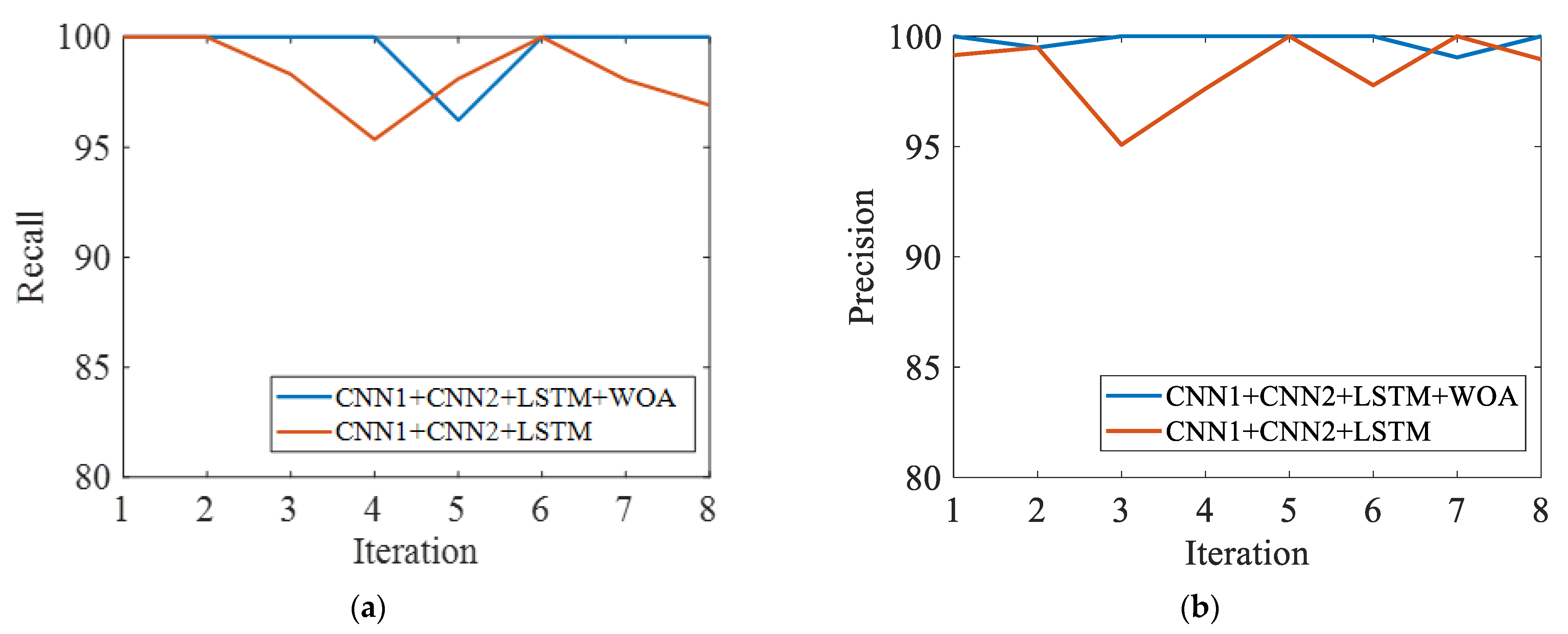
The network with the best recognition effect in Section 3.1.2, which combines CNN1, CNN2 and LSTM, is selected and further optimized by the WOA algorithm. The network performance is presented in Table 2. Through continuous autonomous learning, the accuracy of scene classification is improved from 98.91% to 99.76%, an increase of 0.86%. Macro-F1 is improved from 0.9841 to 0.9967, an increase of 1.28%. The precision and recall of each room are also improved, as displayed in Figure 14.
The parameters obtained after WOA iteration are as follows: the initial learning rate is 0.0126, the L2 regularization is 0.0013 and the LSTM number is 44. The optimized parameters obtained by manual adjustment are different: the initial learning rate is 0.001, the L2 regularization is 0.0003 and the number of LSTMs is 24. The application of WOA significantly reduces the time required for manual tuning. Additionally, it elevates the recognition accuracy and yields a positive impact on scene recognition.

3.2. Results on Public Dataset

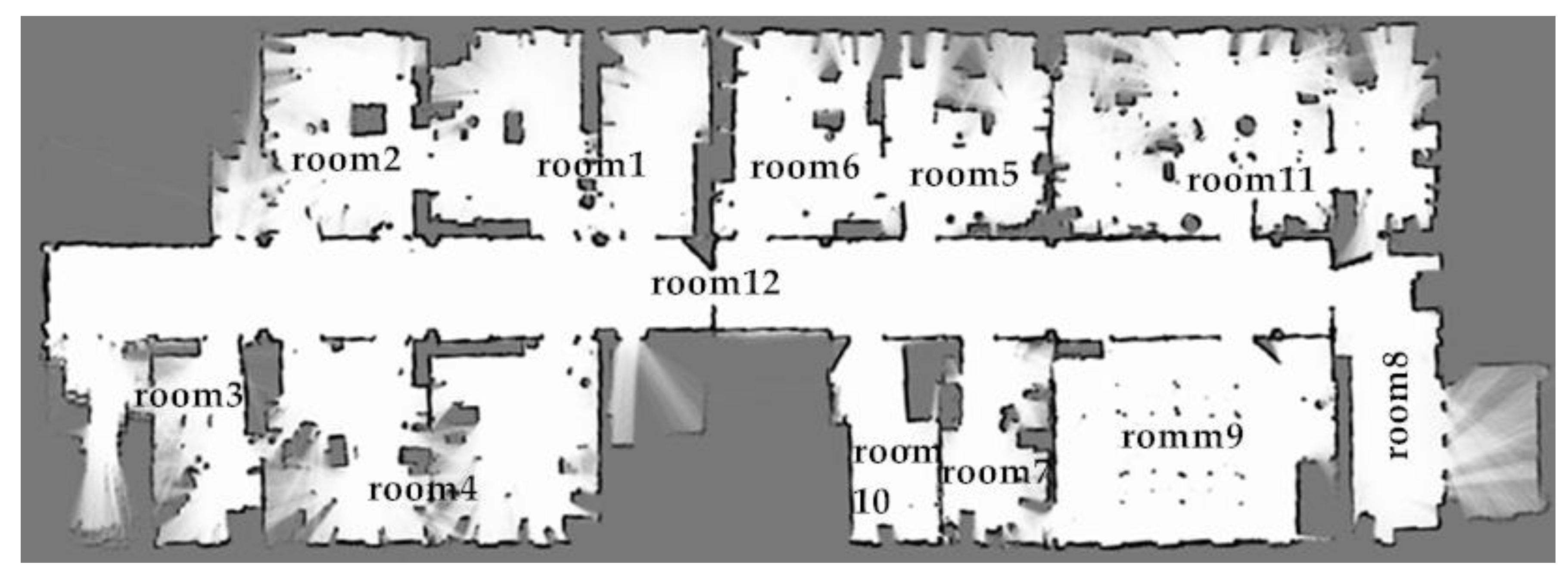
The FR079 public dataset, collected from Building 079 at the University of Freiburg, is employed to assess the proposed network [38]. The dataset contains 3420 frames of LiDAR data, and the map is constructed with an RBPF SLAM algorithm, as shown in Figure 15. It includes a total of 11 rooms and 1 corridor. Room 11 contains the most extensive data with 656 frames, while Room 1 and Room 7 contain the least data with 120 frames. Given the relatively limited data within the FR079 dataset compared to ours, three convolutional layers are added to the proposed network.

3.2.1. Experiments Validation

Before applying WOA optimization, a multi-scale CNN and LSTM fused algorithm is used to classify the 12 rooms in the FR079 dataset. The initial learning rate is 0.001, L2 regularization is 0.0003 and the LSTM number is 64. The classification results are shown in Table 3.
As shown in Table 3, the multi-scale CNN and LSTM fusion algorithm shows a favorable classification effect on the FR079 dataset, with a prediction accuracy of 93.27%, which can meet the classification requirements of the robot. The Macro-F1 reaches 0.9080, proving that the network has a good performance in comprehensive ability.
In order to further improve the accuracy of classification, the WOA algorithm was used to optimize this network, obtaining a updated initial learning rate of 2.99 × 10 4 , L2 regularization of 2.85 × 10 4 and an LSTM number of 118, which improves the accuracy to 94.35%. These parameters are also different from the previously manually set parameters. Therefore, it is verified that the WOA algorithm combined with the proposed network is suitable for the FRO79 dataset, which not only ensures the high classification accuracy, but also reduces the time for manual parameter tuning.
The relationship between the ITC of the WOA algorithm and the number of iterations is shown in Figure 16. The WOA algorithm gradually optimizes the network through iteration; after seven iterations, the network achieves the highest accuracy, and the ITC is close to 0.
Table 4 and Figure 17 presents the classification results of the FR079 dataset. After applying WOA optimization, the accuracy, recall rate and F1 of the network are improved. The accuracy is improved by 1.16% from 93.27% to 94.35%, and Macro-F1 is improved by 2.56% from 0.9080 to 0.9312, demonstrating the applicability of WOA to the FR079 dataset on parameter tuning and performance enhancement.

3.2.2. Comparison of Advanced Algorithms

At present, the classification research of 2D LiDAR semantic maps primarily focuses on classification between categories, such as using AdaBoost to classify rooms, corridors and doors [17], and using deep neural networks to classify corridors, offices, meeting rooms and other rooms [29]. In this paper, classification is refined further. Rather than room category classification, individual rooms with their own serial number are classified to solve the problem of robot localization failure and kidnapping. In contrast, the proposed algorithm has the notable advantage of higher accuracy, at the cost of slightly increased model complexity.
In order to test the performance of the proposed algorithm, it is compared with K-means and MLP algorithms [28]. As for the K-means, when K = 40 and K = 100, the accuracy rates are below 50%, which fails to meet the recognition requirements of the robot. The recognition accuracy rate of the MLP algorithm is 71.44%, which still does not suffice for meeting robot recognition needs or complete the functions of human–computer interaction or kidnapping recovery. The algorithm proposed in this paper can reach 94.35% in accuracy, more suitable for room classification by robots. On the other hand, compared with the advanced methods without the WOA algorithm for optimization, the training parameters and layers numbers of the network need to be set manually. Another advantage of the proposed algorithm is that it does not require manual parameter adjustment to train the network and can automatically obtain the network with the best accuracy. Yet it increases the complexity of the model, as it takes time for continuous network optimization. As can be seen from Table 5, the proposed algorithm takes the longest time of 0.2386 ms for a single prediction, but it is still acceptable for applications of robots’ scene classifications.

4. Conclusions

In this paper, we propose an intelligent optimization method using 2D LiDAR and a CNN network for robot scene recognition. Our method utilizes multi-scale CNN and LSTM to construct a network, and optimizes its parameters using WOA. Firstly, the ablation experiments of networks constructed by different combinations of CNN1, CNN2 and LSTM are conducted with the datasets of eight real-world laboratories. The proposed multi-scale CNN and LSTM networks achieve the best performance. Then, for the FR079 public dataset, the proposed algorithm is compared with other existing advanced algorithms, and the accuracy of the proposed is higher than others. In addition, the ablation experiments of WOA are carried out with both the laboratory and public datasets, verifying that WOA can automatically optimize the network parameters. Experiments show that the proposed method is suitable for indoor robot scene classification using 2D LiDAR.
In the future, the algorithm can be applied to the real-time indoor autonomous navigation of robots, and for indoor robot positioning or repositioning after crash recovery. Compared with room classification methods based on vision, it has two advantages: the first is that minimal data are required, which can reduce the demand for storage units, and the second is that laser data are not affected by lighting conditions or specific requirement for environmental brightness. However, it also has some limitations. In scenes with high similarity, there is a risk of misclassification, particularly in completely consistent office scenes, where additional features may need to be incorporated manually. Thus, we will further utilize the fusion of LiDAR and image data to improve the classification accuracy of symmetrical scenes.

Author Contributions

Conceptualization, X.X. and Y.R.; methodology, Y.R.; supervision, X.X.; validation, Y.R. and M.L.; visualization, Y.R.; writing—original draft preparation, Y.R.; writing—review and editing, X.X., M.L., J.Y. and Z.C. All authors have read and agreed to the published version of the manuscript.

Funding

This research was funded by the Fundamental Research Funds for the Central Universities (grant no. B220202023), and Jiangsu Key R&D Program (grant no. BE2020082-1).

Data Availability Statement

The data presented in this study are available on request from the corresponding author.

Conflicts of Interest

The authors declare no conflicts of interest.

References

  1. Girshick, R.; Donahue, J.; Darrell, T.; Malik, J. Rich Feature Hierarchies for Accurate Object Detection and Semantic Segmentation. In Proceedings of the IEEE Conference on Computer Vision and Pattern Recognition, Columbus, OH, USA, 24–27 June 2014. [Google Scholar]
  2. Girshick, R. Fast R-CNN. In Proceedings of the 2015 IEEE International Conference on Computer Vision, Santiago, Chile, 13–16 December 2015. [Google Scholar]
  3. Ren, S.Q.; He, K.M.; Girshick, R.; Sun, J. Faster R-CNN: Towards Real-Time Object Detection with Region Proposal Networks. IEEE Trans. Pattern Anal. Mach. Intell. 2017, 39, 1137–1149. [Google Scholar] [CrossRef] [PubMed]
  4. Redmon, J.; Divvala, S.; Girshick, R.; Farhadi, A. You Only Look Once: Unified, Real-Time Object Detection. In Proceedings of the 2016 IEEE Conference on Computer Vision and Pattern Recognition, Las Vegas, NV, USA, 26 June–1 July 2016. [Google Scholar]
  5. Liu, W.; Anguelov, D.; Erhan, D.; Szegedy, C.; Reed, S.; Fu, C.Y.; Berg, A.C. SSD: Single Shot MultiBox Detector. In Proceedings of the 2016 European Conference on Computer Vision, Amsterdam, The Netherlands, 11–14 October 2016. [Google Scholar]
  6. Sünderhauf, N.; Pham, T.T.; Latif, Y.; Milford, M.; Reid, I. Meaningful maps with object-oriented semantic mapping. In Proceedings of the 2017 IEEE/RSJ International Conference on Intelligent Robots and Systems, Reykjavík, Iceland, 4–6 January 2017. [Google Scholar]
  7. McCormac, J.; Clark, R.; Bloesch, M.; Davison, A.; Leutenegger, S. Fusion++: Volumetric Object-Level SLAM. In Proceedings of the 2018 International Conference on 3D Vision, Verona, Italy, 5–8 September 2018. [Google Scholar]
  8. Sharma, A.; Dong, W.; Kaess, M. Compositional and Scalable Object SLAM. In Proceedings of the 2021 IEEE International Conference on Robotics and Automation, Xi’an, China, 30 May–5 June 2021. [Google Scholar]
  9. Ni, J.J.; Shen, K.; Chen, Y.N.; Cao, W.D.; Yang, S.X. An Improved Deep Network-Based Scene Classification Method for Self-Driving Cars. IEEE Trans. Instrum. Meas. 2022, 71, 1–14. [Google Scholar] [CrossRef]
  10. Li, Y.; Zhang, Z.; Cheng, Y.; Wang, L.; Tan, T. MAPNet: Multi-modal Attentive Pooling Network for RGB-D Indoor Scene Classification. Pattern Recognit. 2019, 90, 436–449. [Google Scholar] [CrossRef]
  11. Song, X.H.; Herranz, L.; Jiang, S.Q. Depth CNNs for RGB-D scene recognition: Learning from scratch better than transferring from RGB-CNNs. In Proceedings of the Thirty-First AAAI Conference on Artificial Intelligence, San Francisco, CA, USA, 4–9 February 2017. [Google Scholar]
  12. Mosella-Montoro, A.; Ruiz-Hidalgo, J. 2D–3D Geometric Fusion network using Multi-Neighbourhood Graph Convolution for RGB-D indoor scene classification. Inf. Fusion 2021, 76, 46–54. [Google Scholar] [CrossRef]
  13. Zhou, L.G.; Zhou, Y.H.Z.; Qi, X.N.; Hu, J.J.; Lam, T.L.; Xu, Y.S. Attentional Graph Convolutional Network for Structure-Aware Audiovisual Scene Classification. IEEE Trans. Instrum. Meas. 2021, 72, 1–15. [Google Scholar] [CrossRef]
  14. Mochurad, L.; Hladun, Y.; Tkachenko, R. An Obstacle-Finding Approach for Autonomous Mobile Robots Using 2D LiDAR Data. Big Data Cogn. Comput. 2023, 7, 43. [Google Scholar] [CrossRef]
  15. Chen, X.Y.L.; Milioto, A.; Palazzolo, E.; Giguere, P.; Behlcy, J.; Stachniss, C. SuMa++: Efficient LiDAR-based Semantic SLAM. In Proceedings of the 2019 IEEE/RSJ International Conference on Intelligent Robots and Systems, Macau, China, 4–8 November 2019. [Google Scholar]
  16. Kosnar, K.; Vonasek, V.; Kulich, M.; Preucil, L. Comparison of shape matching techniques for place recognition. In Proceedings of the 2013 Europe-an Conference on Mobile Robots (ECMR), Barcelona, Spain, 25–27 September 2013. [Google Scholar]
  17. Mozos, O.M.; Stachniss, C.; Burgard, W. Supervised Learning of Places from Range Data using Adaboost. In Proceedings of the 2005 IEEE International Conference on Robotics and Automation, Barcelona, Spain, 18–22 April 2005. [Google Scholar]
  18. Sousa, P.; Araiijo, R.; Nunes, U. Real-Time Labeling of Places using Support Vector Machines. In Proceedings of the 2007 IEEE International Symposium on Industrial Electronics, Vigo, Spain, 4–7 June 2007. [Google Scholar]
  19. Park, S.; Park, S.K. 2DPCA-based method for place classification using range scan. Electron. Lett. 2011, 47, 1364–1366. [Google Scholar] [CrossRef]
  20. Kaleci, B.; Şenler, Ç.M.; Dutağacı, H.; Parlaktuna, O. A probabilistic approach for semantic classification using laser range data in indoor environments. In Proceedings of the 2015 International Conference on Advanced Robotics, Istanbul, Turkey, 27–31 July 2015. [Google Scholar]
  21. Shi, L.; Kodagoda, S.; Dissanayake, G. Laser Range Data Based Semantic Labeling of Places. In Proceedings of the 2010 IEEE/RSJ International Conference on Intelligent Robots and Systems, Taipei, Taiwan, 18–22 October 2010. [Google Scholar]
  22. Kaleci, B.; Şenler, C.M.; Dutağacı, H.; Parlaktuna, O. Semantic classification of mobile robot locations through 2D laser scans. Intell. Serv. Robot. 2020, 13, 63–85. [Google Scholar] [CrossRef]
  23. Kaleci, B.; Turgut, K.; Dutagaci, H. 2DLaserNet: A deep learning architecture on 2D laser scans for semantic classification of mobile robot locations. Eng. Sci. Technol. 2022, 28, 101027. [Google Scholar] [CrossRef]
  24. Yu, S.K.; Yan, F.; Zhuang, Y.; Gu, D.B. A Deep-Learning-Based Strategy for Kidnapped Robot Problem in Similar Indoor Environment. J. Intell. Robot. Syst. 2020, 100, 765–775. [Google Scholar] [CrossRef]
  25. Goeddel, R.; Olson, E. Learning Semantic Place Labels from Occupancy Grids using CNNs. In Proceedings of the 2016 IEEE/RSJ International Conference on Intelligent Robots and Systems, Daejeon, Republic of Korea, 9–14 October 2016. [Google Scholar]
  26. Nikdel, P.; Chen, M.; Vaughan, R. Recognizing and Tracking High-Level, Human-Meaningful Navigation Features of Occupancy Grid Maps. In Proceedings of the 2020 17th Conference on Computer and Robot Vision, Bangkok, Thailand, 25–28 October 2020. [Google Scholar]
  27. Zheng, T.; Duan, Z.Z.; Wang, J.; Lu, G.D.; Li, S.J.; Yu, Z.Y. Research on Distance Transform and Neural Network Lidar Information Sampling Classification-Based Semantic Segmentation of 2D Indoor Room Maps. Sensors 2021, 21, 1365. [Google Scholar] [CrossRef] [PubMed]
  28. Turgut, K.; Kaleci, B. A Deep Learning Architecture for Place Classification in Indoor Environment via 2D Laser Data. In Proceedings of the 2019 3rd International Symposium on Multidisciplinary Studies and Innovative Technologies (ISMSIT), Ankara, Turkey, 11–13 October 2019. [Google Scholar]
  29. Liao, Y.Y.; Kodagoda, S.; Wang, Y.; Shi, L.; Liu, Y. Place Classification with a Graph Regularized Deep Neural Network. IEEE Trans. Cogn. Dev. Syst. 2017, 9, 304–315. [Google Scholar] [CrossRef]
  30. Ulrich, I.; Nourbakhsh, I. Appearance-based place recognition for topological localization. In Proceedings of the 2000 ICRA. Millennium Conference. IEEE International Conference on Robotics and Automation. Symposia Proceedings (Cat. No.00CH37065), San Francisco, CA, USA, 24–28 April 2000. [Google Scholar]
  31. Lecun, Y.; Bottou, L.; Bengio, Y.; Haffner, P. Gradient-Based Learning Applied to Document Recognition. Proc. IEEE 1998, 86, 2278–2324. [Google Scholar] [CrossRef]
  32. Krizhevsky, A.; Sutskever, I.; Hinton, G. ImageNet Classification with Deep Convolutional Neural Networks. Commun. ACM 2017, 60, 84–90. [Google Scholar] [CrossRef]
  33. Szegedy, C.; Liu, W.; Jia, Y.; Sermanet, P.; Reed, S.; Anguelov, D.; Erhan, D.; Vanhoucke, V.; Rabinovich, A. Going Deeper with Convolutions. In Proceedings of the IEEE Conference on Computer Vision and Pattern Recognition (CVPR), Boston, MA, USA, 7–12 June 2015. [Google Scholar]
  34. Karen, S.; Andrew, Z. Very Deep Convolutional Networks for Large-Scale Visual Recognition. In Proceedings of the 2015 International Conference on Learning Representations, San Diego, CA, USA, 7–9 May 2015. [Google Scholar]
  35. He, K.M.; Zhang, X.Y.; Ren, S.Q.; Sun, J. Deep Residual Learning for Image Recognition. In Proceedings of the 2016 IEEE Conference on Computer Vision and Pattern Recognition, Las Vegas, NV, USA, 26 June–1 July 2016. [Google Scholar]
  36. Hochreiter, S.; Schmidhuber, J. Long short-term memory. Neural Comput. 1997, 9, 1735–1780. [Google Scholar] [CrossRef] [PubMed]
  37. Seyedali, M.; Andrew, L. The Whale Optimization Algorithm. Adv. Eng. Softw. 2016, 95, 51–67. [Google Scholar]
  38. Abdelmunim, H.; Farag, A.A. Elastic Shape Registration using an Incremental Free Form Deformation Approach with the ICP Algorithm. In Proceedings of the 18th IEEE International Conference on Image Processing, Brussels, Belgium, 11–14 September 2011. [Google Scholar]
Figure 1. Coordinate system transformation: (a) polar coordinate system; (b) rectangular coordinate system; (c) range sequence coordinate system.
Remotesensing 16 00174 g001
Figure 2. Data sequence of different frames in Room 1: (a) the 1st frame; (b) the 150th frame.
Remotesensing 16 00174 g002
Figure 3. Data sequence of different frames in Room 2: (a) the 1st frame; (b) the 150th frame.
Remotesensing 16 00174 g003
Figure 4. Network structure.
Remotesensing 16 00174 g004
Figure 5. Several frames of data in Room 4.
Remotesensing 16 00174 g005
Figure 6. The dual-scale CNN.
Remotesensing 16 00174 g006
Figure 7. LSTM framework.
Remotesensing 16 00174 g007
Figure 8. Experimental platform.
Remotesensing 16 00174 g008
Figure 9. The 80th frames of the 2D LiDAR data: (a) Room 1; (b) Room 2; (c) Room 3; (d) Room 4; (e) Room 5; (f) Room 6; (g) Room 7; (h) Room 8.
Remotesensing 16 00174 g009aRemotesensing 16 00174 g009b
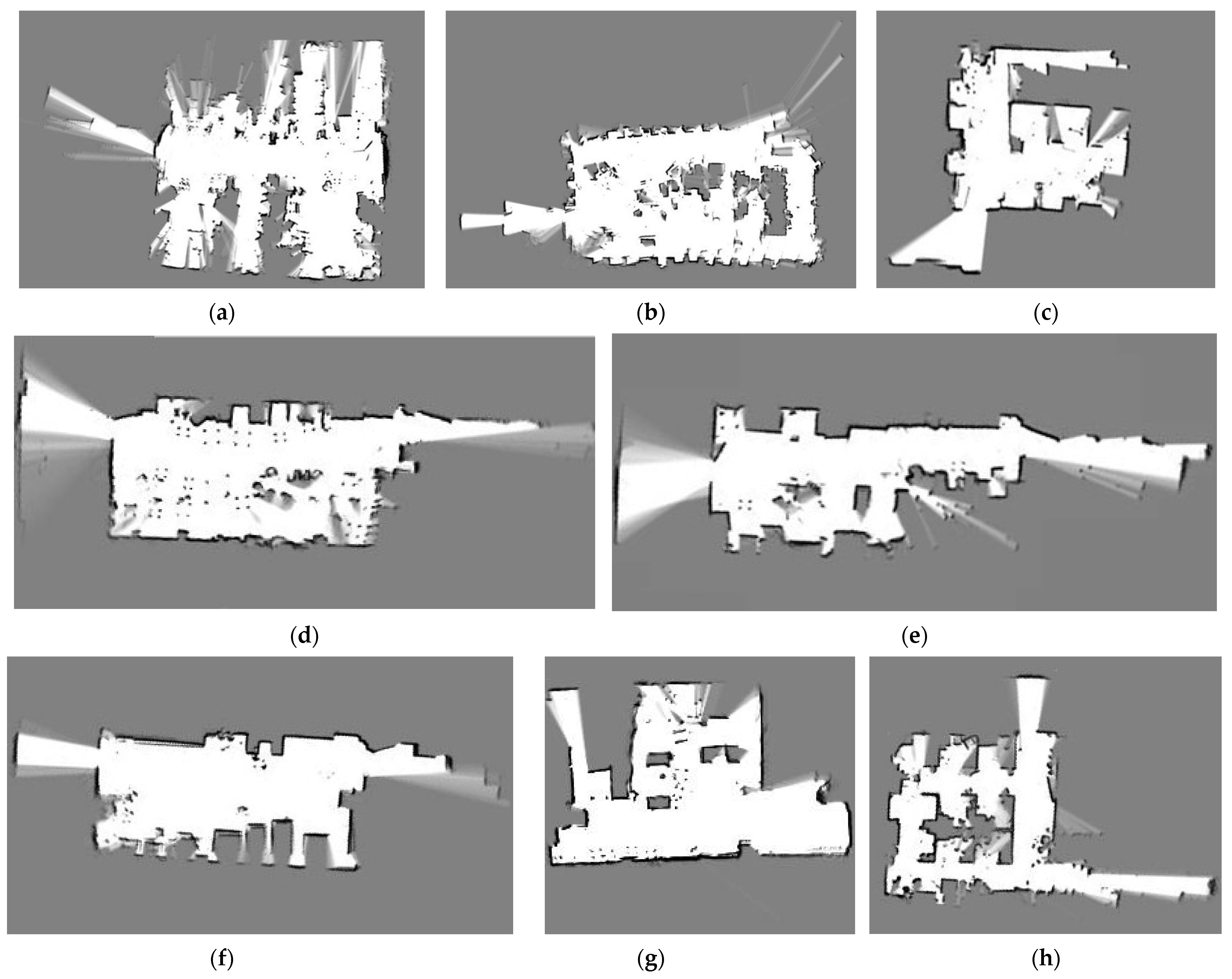
Figure 10. Cartographer mapping in (a) Room 1; (b) Room 2; (c) Room 3; (d) Room 4; (e) Room 5; (f) Room 6; (g) Room 7; (h) Room 8.
Remotesensing 16 00174 g010
Figure 11. Content of ablation experiment.
Remotesensing 16 00174 g011
Figure 12. Performance comparison of different algorithms: (a) recall curve; (b) precision curve; (c) F1 curve; (d) Macro-F1 curve.
Remotesensing 16 00174 g012
Figure 13. The relationship between ITC and iteration number for the WOA algorithm in laboratory dataset.
Remotesensing 16 00174 g013
Figure 14. The effect of WOA on the network: (a) recall rate comparison; (b) precision rate comparison.
Remotesensing 16 00174 g014
Figure 15. Drawing of FR079 dataset with rooms and corridors marked.
Remotesensing 16 00174 g015
Figure 16. The relationship between ITC and iteration number for the WOA algorithm in FR079 public dataset.
Remotesensing 16 00174 g016
Figure 17. The effect of WOA in the FR079 dataset: (a) precision comparison; (b) recall comparison; (c) F1 comparison.
Remotesensing 16 00174 g017
Table 1. Results of different algorithms.
CNN1CNN1 + CNN2CNN1 + LSTMCNN1 + CNN2 + LSTM
Accuracy (%)92.4495.5698.3098.91
Macro-F10.91020.9525 0.98040.9841
Ttotal/s114.00147.00117.00152.40
Tprediction/ms0.10360.11960.10780.1236
Table 2. Network performance.
Room 1Room 2Room 3Room 4Room 5Room 6Room 7Room 8
Accuracy (%)98.87
Precision (%)98.8599.1598.8697.6496.7999.2598.3797.66
Recall (%)99.4298.6497.7496.1295.5799.2597.73100.00
F10.98990.98550.99150.98420.96880.98880.99510.9966
Macro-F10.9876
Table 3. Network performance parameters.
Room 1Room 2Room 3Room 4Room 5Room 6
Accuracy (%)93.27
Precision (%)80.00100.0092.3183.8793.0595.65
Recall (%)100.0084.6285.7186.6791.3095.65
F10.88890.91670.88890.85250.92170.9565
Macro-F10.9080
Room 7Room 8Room 9Room 10Room 11Room 12
Accuracy (%)93.27
Precision (%)84.6281.8293.0294.7495.4597.44
Recall (%)91.6769.2397.5090.0094.42100.00
F10.88000.75000.95210.92310.94930.9870
Macro-F10.9080
Table 4. WOA optimized network performance parameters.
Room 1Room 2Room 3Room 4Room 5Room 6
Accuracy (%)94.35
Precision (%)91.6786.84100.0094.5793.0691.04
Recall (%)91.6785.7193.4896.6797.1087.14
F10.91670.86270.95000.95600.95040.8905
Macro-F10.9312
Room 7Room 8Room 9Room 10Room 11Room 12
Accuracy (%)94.35
Precision (%)90.91100.0091.6091.9496.8697.93
Recall (%)83.3389.7497.5696.6194.8799.47
F10.86960.94590.94490.94210.95850.9869
Macro-F10.9312
Table 5. Algorithm accuracy comparison in dataset.
K-Means, K = 40 [20]K-Means, K = 100 [20]MLP [28]Proposed Method
Accuracy (%)43.3745.7171.4494.35
Tprediction/ms0.08790.11670.19910.2386
Disclaimer/Publisher’s Note: The statements, opinions and data contained in all publications are solely those of the individual author(s) and contributor(s) and not of MDPI and/or the editor(s). MDPI and/or the editor(s) disclaim responsibility for any injury to people or property resulting from any ideas, methods, instructions or products referred to in the content.