Article

Uncovering Plastic Litter Spectral Signatures: A Comparative Study of Hyperspectral Band Selection Algorithms

by
Mohammadali Olyaei
* and
Ardeshir Ebtehaj
Department of Civil, Environmental and Geo-Engineering, University of Minnesota, Minneapolis, MN 55455, USA
*
Author to whom correspondence should be addressed.
Remote Sens. 2024, 16(1), 172; https://doi.org/10.3390/rs16010172
Submission received: 28 November 2023 / Revised: 28 December 2023 / Accepted: 29 December 2023 / Published: 31 December 2023
(This article belongs to the Section AI Remote Sensing)

Abstract

:
This article provides insights into the optical signatures of plastic litter based on a published laboratory-scale reflectance data set (350–2500 nm ) of dry and wet plastic debris under clear and turbid waters using different band selection techniques, including sparse variable selection, density peak clustering, and hierarchical clustering. The variable selection method identifies important wavelengths by minimizing a reconstruction error metric, while clustering approaches rely on the strengths of the correlation and local density of the spectra. Analyses of the data reveal three distinct absorption lines at 560, 740, and 980 nm that produce relatively broad reflectance peaks in the measured spectra of wet plastics around 475–490, 635–650, 810–815, and 1070 nm . The results of band selection consistently identify three important regions across 450–470, 650–690, and 1050–1100 nm that are close to the reflectance peaks of the mean of wet plastic spectra over clear and turbid waters. However, as the number of isolated important wavelengths increases, the results of the methodologies diverge. Density peak clustering identifies additional wavelengths in the short-wave infrared (SWIR) region of 1170–1180 nm ) as a result of a high local density of the reflectance points. In contrast, hierarchical clustering isolates more wavelengths in the visible range of 365–400 nm due to weak correlations of nearby wavelengths. The results of the clustering methods are not consistent with the visual inspection of the signatures as peaks and valleys in the spectra, which are effectively captured by the variable selection method. It is also found that the presence of suspended sediments can (i) shift the important wavelength towards higher values in the visible part of the spectrum by less than 50 nm , (ii) attenuate the magnitude of wet plastic reflectance by up to 80% across the entire spectrum, and (iii) manifest a similar spectral signature with plastic litter from 1070 to 1100 nm .

1. Introduction

Plastic pollution in oceans, rivers, and lakes is becoming an important environmental concern with negative impacts on human health and socioeconomic sustainability [1]. In marine ecosystems, plastic currently constitutes more than 80–90% of all litter. This problem is expected to exacerbate under the current trends of social practices, wherein the annual production of plastic waste could reach more than 50 million metric tons by 2030 [2].
Even though new strategies for plastic production, use, and recycling are needed to mitigate its environmental pollution [3], new technologies are critical for their cost-effective interception, especially in aquatic environments. The conventional methods for detecting floating plastics are through in situ collection by deploying net trawls and sea bins. While these methods are always necessary for acquiring reliable information about the physical characteristics of the debris, they are labor-intensive and time-consuming [4]. Remote sensing has the potential to improve monitoring and accelerate cost-effective interception, as well as support the removal of floating plastic litter in aquatic environments [5].
Research to understand the spectral properties of plastic litter has been either conducted in laboratories or the field [6]. The former approach often focuses on understanding the spectral reflectance signatures of plastics in the visible to near-infrared (VNIR) and short-wave infrared (SWIR) regions of the spectrum [7,8,9] through laboratory-scale measurements using hyperspectral spectroradiometers. The latter approach often relies on observations from various remote sensing platforms such as satellites, aircraft, and unmanned aerial vehicles (UAVs) equipped with passive and active sensors [10,11].
Through visual inspection, previous laboratory studies of virgin and weathered plastics under dry and wet conditions revealed some absorption features from VNIR to SWIR wavelengths around, for example, 930 nm , 1045 nm , 1215 nm , 1732 nm , and 2046 nm [12]. These studies also demonstrated that the reflectance in the SWIR region can be masked [13] due to strong water absorption [6]. Clearly, the detection of floating plastic litter in actual water bodies is much more challenging than in a controlled environment [13] due to background contamination of the spectral signatures in the presence of atmosphere and other optically active floating materials such as algal biomass, whitecaps, and waves [14].
Airborne and satellite multispectral imageries have been used, especially over marine environments [2], such as those from the Sentinel-2 satellite [15,16,17] for the detection of plastic litter in aquatic environments. Additionally, there exist studies that used X-band [18] and synthetic aperture radar (SAR) data [19] for marine debris detection. The MultiSpectral Instrument (MSI) onboard Sentinel-2 provides reflectance with a spatial resolution of 10–60  m at 13 spectral bands from visible to SWIR bands [20]. Machine learning techniques [15,16,21,22] or spectral indices [20,21,23,24,25,26] have been deployed to detect and classify the types of the marine debris from MSI observations. However, currently, there exists no specific multispectral spaceborne sensor that is optimally designed for the detection of plastics in the aquatic environment.
The problem of selecting important frequency bands is imperative because hyperspectral remote sensing is expensive, especially from space, and may contain redundant information when the detection of plastics is concerned [27]. The key questions that this paper aims to address are as follows: What are the optimal central wavelengths, in VNIR-SWIR, that can capture the occurrence and respond to different types of plastics? What is the optimal number of wavelengths necessary for designing an effective optical remote sensing platform? How can suspended sediments affect the spectral signatures? Providing answers to these questions relies on high-quality hyperspectral reflectance data of various plastic types and underlying environmental conditions. Recently, there have been laboratory-scale efforts [13,14,28] to collect hyperspectral data of wet and dry plastic reflectance across 350–2500 nm . The goal of this paper is to learn from these new data sets and to answer the posed questions, thereby depending on the representativeness and limitation of the data through a few band selection approaches.
In the literature, various classes of hyperspectral band selections have been developed for different applications, including environmental monitoring [29], medical imaging [30], and biological analysis [31]. These methods often rely on statistical variable selection [32], ranking techniques [33], clustering methods [34], and various optimization techniques that identify the best band combination based on an optimality criterion [35].
Here, unlike previous research that mainly relied on visual inspection [14,28] of the data set of plastic litter spectral measurements, to uncover the spectral signatures, we compare the outcomes of three different unsupervised band selection methods, including the probabilistic sparse variable selection method [36,37], the unsupervised density peak clustering (DPC) method [38], and the hierarchical clustering [34] method. The sparse decomposition method, using the least angle selection and shrinkage operator (LASSO) regression [39], is a well-established method as a statistical variable selection approach and is used in the field of remote sensing for optimal band selection [40,41]. Here, this technique is used to approximate the plastic spectra with a few triangular basis functions whose positions identify the location of important wavelengths.
Clustering methods have been employed for hyperspectral imaging band selection by grouping bands into clusters and selecting a representative band in each cluster. Usually, the clustering methods are derived from k-means [42], affinity propagation (AP) [43], density [44] and graph-based [45] clustering methods. The representative band in each cluster is usually selected based on the maximum information it can provide such as the selection based on maximum variance [34], entropy [46], or mutual information [47]. This family of band selection methods rests on the idea that the spectral signatures form clusters of nearby points. Inspired by methodologies used for identifying brain signals [48] and important gene selection [49], we apply the clustering approach to the correlation matrix of the observed spectra because it can capture which part of the spectrum would respond in the form of synchronized reflectance peak and absorption valleys in response to the presence of plastic litter in the field of view of the spectroradiometer.
This article is organized as follows. Section 2 describes the data, the methodology, and explains the details of all three methods. The results and discussions are presented in Section 3 and Section 4, followed by the concluding remarks in Section 5.

2. Materials and Methods

2.1. Data

We used a publicly available hyperspectral reflectance data set of various aquatic and marine litter types provided in [13]. Data were acquired utilizing an analytical spectral device (ASD), FieldSpec 4, and a Spectral Evolution (SEV) spectroradiometer. The spectral ranges of both spectroradiometers are relatively similar, with the ASD covering the interval from 350 to 2500 nm and the SEV sampling from 295 to 2484 nm . However, the spectral resolutions are not uniform throughout the spectrum. The ASD (SEV) has a higher resolution of 3 (4) nm for wavelengths smaller than 1000 nm , while in the SWIR region, the resolution varies from 10 to 12 (7 to 10) nm . These spectral resolutions and postprocessing methodologies result in 2151 bands recorded in the ASD and 2190 recorded in the SEV measurements. The foreoptic field of view (FOV) was maintained constant at 8 across all measurements. The data set contains ASD measurements of 47 litter types with 151 spectral samples of virgin and weathered plastics. The SEV measurements include 64 samples of 4 different virgin plastic litter types. The list of samples for each spectroradiometer is shown in Table 1; the examples of mean spectra of placemats and ropes with different colors are shown in Figure 1. The experiments were conducted on dry, wet, and submerged samples, with two levels of concentrations for suspended sediments at 75 and 321 mg   L 1 , which were presented in a water tank with a dimension of 2 m in diameter and 3 m in depth. Samples of ropes and placemats were placed at different depths (i.e., 0, 2.5, 5, 9, 12, 16, and 32 cm).
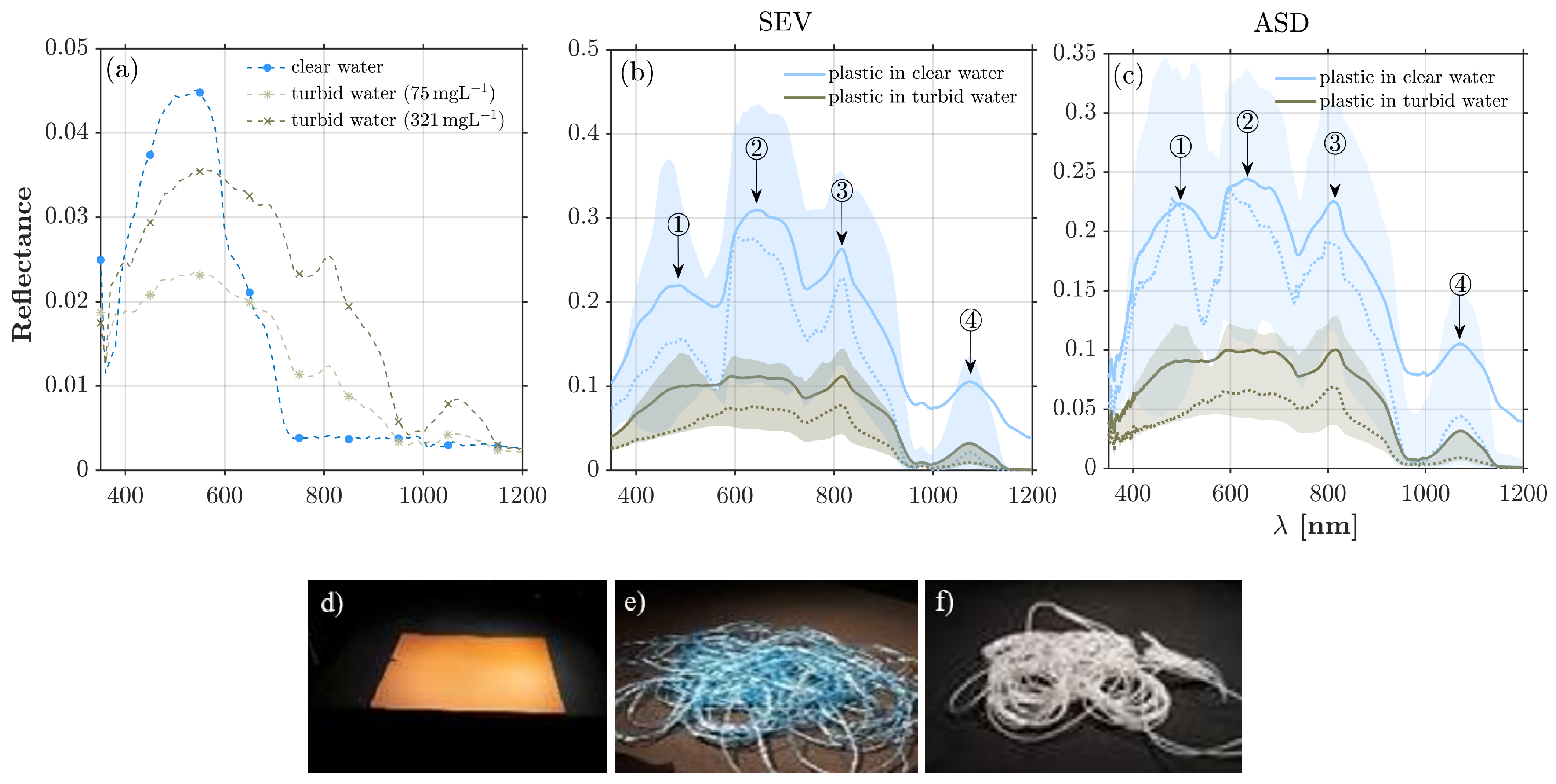
The mean spectra of clear and turbid water with two levels of concentrations are shown in Figure 2a. The peak reflectance in the clear water spectrum was around 540  nm and was shifted by ∼10  nm towards higher wavelengths for turbid waters. While the high reflectivity of clear waters near the red region of the spectrum was reported in the previous literature [50,51], the precise wavelengths of absorption features differ, perhaps due to different dissolved optically active constituents among the tested samples. For example, the SeaSWIR data set [52], which comprises 97 seawater reflectance spectra, shows a range of maximum reflectance varying from 570 to 810 nm . The analyzed data in this study indicate that turbid waters are more reflective at longer wavelengths than clear waters, and extra reflectance peaks manifest themselves at around 810 and 1070 nm as the concentration of suspended sediments increases. This observation is consistent with SeaSWIR data set reporting local reflectance peaks in the NIR region at 760–815 and SWIR region at 1000–1150  nm ) for turbid waters.
Figure 2b,c represent the mean spectrum of wet plastics in the clear and turbid waters from data collected by SEV and ASD, respectively. In general, the reflectance was similar for both devices and significantly higher for clear water samples. For plastics in clear waters, the mean spectra had a few main reflectance peaks centered around 475 (490), 650 (635), 815 (810), and 1070 (1070) nm in the SEV (ASD) data. The reflectance peaks had closer magnitudes in the ASD data than in the SEV data. As is evident, in turbid waters, there was an almost 80% reduction in the reflectance of plastic compared to clear water due to the absorption of light by the sediment particles. The spectrum in this case did not show a distinct peak in the visible range, but there were two distinct maxima centered around 815 and 1070 nm for both data sets. In other words, it appears that when water is turbid, the absorption valleys are negligible in the visible range. It is important to note that the peak reflectance at (NIR) 815 and (SWIR) 1070 nm occurred due to the presence of both suspended sediments with high concentration and plastic debris. In the data sets, as most of the wet samples were (partially) submerged, no signature was observed over wavelengths greater than 1200 nm due to strong water absorption.

2.2. Sparse Variable Selection

Sparse approximation problems have been studied for several years in numerous applications in image processing, computer vision, machine learning, denoising, and regularization [53]. The goal is to represent a given signal as a linear combination of a few numbers of basis functions [54]. In mathematical terms, let us assume that A R n × m is a dictionary in the form of a fat matrix ( n m ) representing an under-determined system of linear equations y = A x containing a set of basis functions in its column space that a linear combination of a few of them can reconstruct the observation y R n . In other words, the solution x = ( x 1 , x 2 , , x m ) T R m is sparse and has only a few nonzero elements. A computationally efficient solution is through using the class of greedy approaches such as the orthogonal matching pursuit (OMP, [55]), which attempts to iteratively reconstruct the observation through a linear combination of k m number of suboptimally selected columns of A —either for a fixed number of k or based on a minimum error criterion.
For the problem at hand, y R n is the measured reflectance at n central wavelengths, and A is a dictionary in which the observed spectrum should exhibit a sparse representation. The key question here is how to construct a dictionary that leads to a probabilistic band selection by isolating informative regions of the spectrum. In spectral analysis, often the peak reflectance values and abrupt transitions in a spectrum encode the most informative wavelengths responding to the presence of specific materials (e.g., green vegetation, snowpack, plastics) within the FOV. To capture the peaks and valleys here, we consider triangular basis functions that can be empirically obtained from a set of training examples of observed spectra. To clarify this concept, Figure 3a–c show sparse reconstructions of the entire spectrum of a dry orange placemat in the data set with different degrees of sparsity. As shown, when sparsity is equal to one ( k = 1 ), first a triangle basis with the highest correlation with the spectrum is identified (gray dash-dot line) and properly scaled to result in a least-squares reconstruction error. As the sparsity increases to k = 3 and 6, the reconstruction error shrinks, and additional triangular basis functions are selected from the dictionary, where the location of their apexes (red dashed lines) isolates important wavelengths.
To test the aforementioned hypothesis, we produced a large and redundant number of triangular basis functions from a training set. Each triangular basis can be constructed by linearly connecting the beginning and the end of the observed spectra to a randomly sampled midpoint. Specifically, we randomly sampled the observed spectrum of the orange placemat y R n at M = 1000 midpoints to generate a matrix A = [ a 1 | a 2 | | a M ] R n × M , where { a m } m = 1 M represents the mth triangle basis at n number of wavelengths. Then, we minimized the following regularized least-squares problem using OMP for k = 1 , 3 , 6 basis functions:
minimize x y A x 2 2 s . t . x 0 k ,
where x 2 2 denotes the 2 norm or sum of squares, and the zero norm denotes the number of nonzero elements. We repeated this reconstruction for a large number of observed spectra to identify the probability distribution of apexes of the basis functions for which the modes identify the most informative regions of the spectrum concerning the occurrence of various plastic debris. A pipeline of the presented method is shown in Algorithm 1. Since the number of samples was limited, we employed 10-fold crossvalidation to effectively utilize the information content of the entire dataset for training and validation. As is evident, the important wavelengths with this method can be identified probabilistically, thereby enabling uncertainty quantification.
Algorithm 1: Sparse Variable Selection for Probabilistic Identification of Important Wavelengths Capturing the Spectral Signatures of Plastic.
Remotesensing 16 00172 i001

2.3. Clustering Approach

The clustering approach in the family of band selection methods seeks to remove spectral redundancy while preserving the informative spectral regions [47]. As explained, clustering with respect to the correlation matrix has been employed for different applications, for example, in biology [56], image segmentation [57], identification of dominant genetic variants [49], and the detection of brain regions exhibiting similar behavior between resting and attentive states [48]. Inspired by these studies, in the context of plastic litter, the two clustering techniques were applied to the wavelengths correlation matrix to pinpoint segments of the spectrum that exhibited coherent absorption or reflection in response to the presence of plastic litter in the field of view (FOV). To be self-content, the subsequent sections provide a summary of the two clustering methods, including density peak clustering and hierarchical clustering.

2.3.1. Density Peak Clustering

The density peak clustering (DPC, [38]) algorithm rests on the conceptual assumption that clusters contain data points with high local densities, while the centers of those clusters need to be separated from each other considerably. In general, simple parameterization and the ability to deal with nonspherical clusters are the main advantages of this method [58]. To identify the cluster centers, two quantities are computed for each data point i. First, a local density ρ i is computed. This density parameter measures how many data points are centered around the data point and is typically estimated using a Gaussian kernel as follows:
ρ i = j exp d i j 2 d c 2 ,
where d i j is the Euclidean distance between point i and j, and d c is a cutoff distance. The cutoff distance is set to ensure that the average number of neighbors falls within the range of approximately 1 to 2% of the total number of points in the dataset, as recommended in [38].
The second quantity is δ i , which quantifies the minimum distance of the point i with any other points j with a higher density, and it is defined as follows:
δ i = min j ( d i j ) , j : ρ j > ρ i max j ( d i j ) , otherwise .
The pair of ρ and δ for each cluster, in the so-called decision graph, enables the isolation of separated clusters of points with a sufficiently high density, where both parameters are relatively high. Those high-density clusters with relatively small δ are close to another cluster and do not contain unique information. When the relative density (distance) is low (high), the data points are not densely clustered and are far apart from other identified clusters.

2.3.2. Hierarchical Clustering

Conceptually, the unsupervised agglomerative hierarchical clustering method [59] initially considers each data point as a single cluster and then, based on a proximity measure, merges the nearby clusters iteratively through greedy approaches [60] until a predefined stopping criterion is met. The stopping criteria can be a predefined number of clusters or a specific distance threshold between the clusters [61]. In general, two parameters need to be determined: first the distance function between two data points and second the linkage criterion, which measures the distance between two clusters. Usually, the Euclidean distance is used for measuring proximity between the data points [62]. In this study, the proximity of two clusters was quantified using the mean pairwise Euclidean distance between all points in the clusters [63].
To implement this approach in the correlation domain, the distance was defined as 1 minus correlation coefficients, and the clustering approach was applied to columns or rows of the correlation matrix [48]. Throughout the merging process, the relationship between the clusters is represented by a dendrogram, which provides a visual representation of how data points are clustered. Using the dendrogram and a given cutoff threshold, the number of desired clusters are determined, and the centers of clusters in the correlation domain are considered as important wavelengths.

3. Results

In this section, we first present the results of the band selection based on the sparse variable selection method to obtain the probability density functions (pdfs) of important wavelengths. Next, we provide the important wavelengths identified through density peak clustering and hierarchical clustering. Finally, we discuss the practical implications of leveraging these important wavelengths in the domain of multispectral remote sensing. To facilitate the forthcoming discussion, we use the following acronyms: VIS ( λ < 750   nm ), NIR ( 750 λ < 1000   nm ), and SWIR ( 1000 λ 2500   nm ), which are defined as recommended in [64].

3.1. Important Wavelengths via Sparse Variable Selection

Figure 4a,b represents the p Λ ( λ c ) (Algorithm 1) for all wet plastics in turbid and clear water collected by both the SEV and ASD spectroradiometers, respectively. All the samples in turbid waters were analyzed in one set, irrespective of the concentration of the suspended sediments, to cope with a limited sample size. In both cases, the sparsity was increased from k = 1 to 5, and the pdfs were constructed using the nonparametric kernel density estimation method [65] by setting the kernel width to 50 nm .
For k = 1 , the mode of the pdf manifested itself around 650 and 680 nm for clear and turbid waters, respectively, which is consistent with the location of reflectance peak values in Figure 2. It is important to note that the color of plastic samples was also dominated by orange (i.e., placemats and ropes), which can have a significant reflectance around 600 nm . Thus, the signature might be partially due to the distribution of the color of the samples. The observed shift in the identified location of important wavelengths in turbid water also seems to corroborate with the results in Figure 2—the background turbid water was more reflective over the NIR region and thus could shift the total reflectance slightly toward longer wavelengths. It should be noted that there were two primary distinctions between the distribution of the important wavelengths based on SEV and ASD data.
First, the ASD pdf was less concentrated around the mode and had a larger width. Second, for the SEV data, another mode with a lower frequency of occurrence manifested itself around 820 nm . These differences can be explained by visual inspection of the mean spectra in Figure 1b,c. The distribution of the reflectance in the SEV data seems to be more kurtotic. In other words, the mean peak reflectance values in the ASD data are relatively at the same magnitude, while the second peak in the SEV data is appreciably larger than the other peaks. Thus, the algorithm selected peaks 1 and 3 with almost equal probability in a few ASD samples, thereby making its distribution wider around the mode compared to the SEV counterpart. However, the second mode of p Λ ( λ c ) at 820 nm in the SEV data implies that the algorithm selected this wavelength (third peak in Figure 1b) more frequently than those wavelengths around peak 1. Overall, based on the information content of the data sets, the results indicate that the wavelengths around 650–680 and 820 nm are the most important wavelengths for the reconstruction of the wet plastic spectrum and can be essential for its detection using optical remote sensing.
Increasing the number of basis functions to k = 2 , an additional mode manifested itself around 1100 nm for reflectance measurements over clear waters in both data sets. However, this signature was relatively obscured in turbid waters. It is important to note that, as shown in Figure 2a, the peak reflectance around 1100 nm in turbid waters can be due to the suspended sediments [51]. Despite the previous notions that water reflectance in the SWIR region is negligible, known as the black pixel assumption, recent research showed that, in turbid water, this assumption may not be necessarily true [66], particularly at 1070 nm , where there is a local minimum in the water absorption spectra [67,68]. In other words, both plastic and sediment particles can reflect around this wavelength, and their signatures can be mixed. Unlike the p Λ ( λ c ) value for the SEV data, there existed additional modes at 450 (for both clear and turbid water) and 850 nm (only for turbid water) in the pdf derived from the ASD data. This observation implies that for k = 2 , the first and third reflectance peaks (Figure 2b,c) contribute more frequently in the reconstruction of the spectrum using the ASD data than in the SEV data—especially over turbid waters. This difference can be due to the different sample types and sizes in the studied data sets. Since the sample size in the ASD data was larger, it is reasonable to believe that the extra modes in the ASD data represent meaningful information beyond what can be deduced from the the SEV data. Overall, the top-two important wavelengths are around 650–680 and 1070–1100 (850) nm in clear (turbid) waters.
By further increasing the number of the involved basis functions to k > 2 , the shape of p Λ ( λ c ) manifested multiple modes and became relatively insensitive to the increased water turbidity. More importantly, the number and position of the modes stabilized and did not change markedly as a function of k. This assertion was verified through the application of the Wasserstein distance [69,70,71] as a metric to quantify the dissimilarity between the pdfs of clear and turbid waters. It is observed that this distance metric between the pdfs dropped by more than 60% as k increased from one to five. Specifically, for k > 5 , the modes for clear water spectra were located around 455 (450), 650 (645), 820 (830), and 1095 (1100) nm for the SEV (ASD) data. The presence of suspended sediments appeared to shift the mode to longer (shorter) wavelengths by less than 50 nm over the VNIR (SWIR) regions of the spectrum. The shift in the SWIR range is possibly caused by the peak of turbid water reflectance around 1070 nm [51]. It is worth noting that the location of these important wavelengths can be influenced by several factors, including the sample’s color, material, and water spectrum. While the impact of the color of the samples is largely felt in VIS, the interaction between the water and material spectra manifests itself over the NIR and SWIR regions at values greater than 900 nm , depending on the type of the material [6,14].
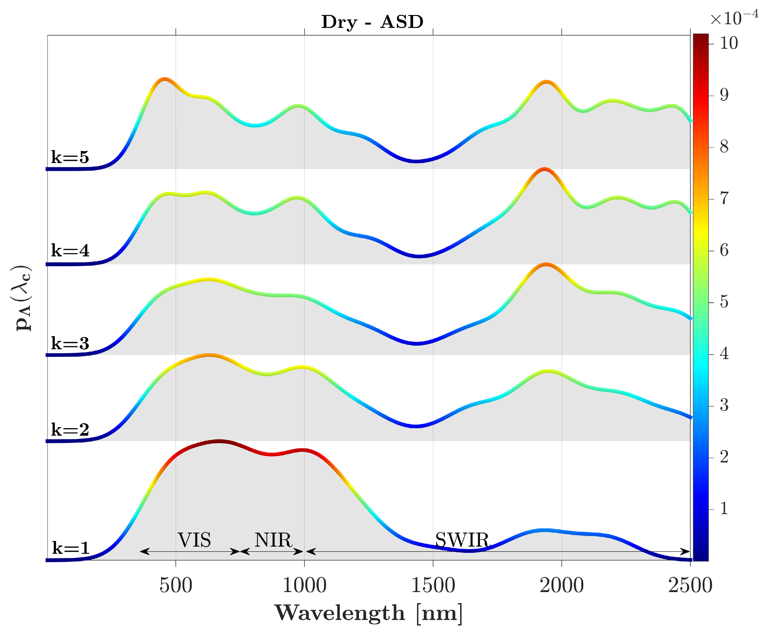
For dry plastics, the pdf of the important wavelengths is shown in Figure 5, which expectedly extended to 2500 nm due to the lack of water absorption. Visual inspection shows, for k = 1 , that the pdf does not have any distinct and isolated modes but rather the highly probable wavelengths are spread over the VIS and NIR bands from 400 to 1100 nm . This can be associated with the mixture of reflectance due to the different colors of the sampled plastic litter. When two important wavelengths are sought (i.e., k = 2 ), those wavelengths around 1800 nm manifest themselves as a secondary mode reflecting the characteristic of the materials. As sparsity increases and more wavelengths become involved, the role of the SWIR region from 1700 to 2000 nm becomes more pronounced. This is in line with previous research that has identified significant absorption features in this spectral range for different types of plastic polymers [14]. However, the modality of the pdf did not change significantly as k increased, and it appears that there are four important regions centered around 455, 630, 980, and 1800 nm . Further studies with larger data sets that include plastics with different polymer types (e.g., terephthalate, polypropylene, polyester, and low-density polyethylene) are felt to be needed in order to make a more robust conclusion concerning the dry plastics, as recent drone-based surveys have demonstrated promising results in dry beach litter categorization [72,73].
To make a collective inference based on all the available data, we applied the methodology to the entire data set of wet plastics obtained from both spectroradiometers, irrespective of the background water turbidity. The central wavelengths of the identified modes and their uncertainty values are shown with light blue circles in Figure 6. The results show that, as the number of wavelengths increased, the location of the modes converged to a few central wavelengths, and the width of the density around the modes shrank. Visual inspection of the mean spectra (Figure 2b,c) indicates that the algorithm first captured the reflectance peaks and then gradually engaged the absorption valleys as the number of important wavelengths increased. In particular, the top four important wavelengths eventually converged to 455, 650, 820, and 1100 nm , which are around the peak reflectance values. As the sparsity k increased to seven, we can see that the locations of the absorption valleys manifested themselves through three modes at wavelengths of 555, 745, and 975 nm . It is important to note that the number of modes of p Λ ( λ c ) remained invariant with respect to the number of selected basis functions for k 13 .

3.2. Important Wavelengths via Density Peak Clustering

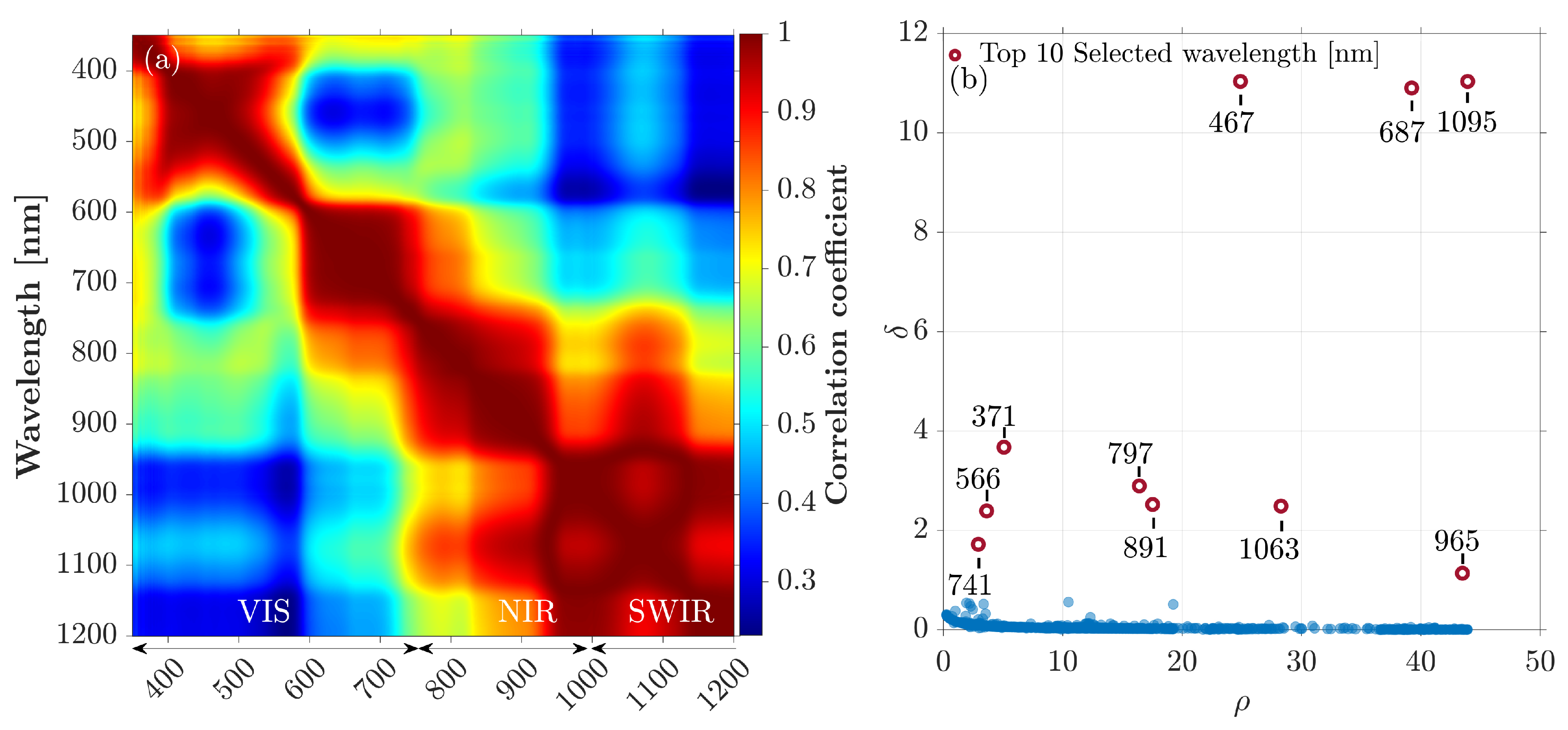
Figure 7a shows the correlation matrix of the reflectance values of wet plastic litter using augmented data from both spectroradiometers. As shown, in the VIS range, the correlation length of the reflectance values was at its maximum around 450 nm (blue bands) and at its minimum around 600 nm (red bands). The correlation length increased as the wavelength increased and became a maximum within the NIR and SWIR ranges. The observed pattern is consistent with the physics of the problem. In the visible range, where the reflectance data respond to the incoherent reflection of plastic litter, the correlation length will be shorter contrary to longer wavelengths, where the spectral response is minimal due to high water absorption.
Figure 7b shows the decision graph based on the wet plastic spectral reflectance utilizing the DPC algorithm. To have a robust method for selecting points with high values of ρ and δ , we first rescaled the points in the decision graph through standard normalization and subsequently ranked the centers of the clusters based on their Euclidean distances from the origin to obtain those clusters that were dense enough and were far apart from each other. Within this graph, the top-10 wavelengths that had the maximum distance from the origin are shown with their corresponding wavelengths. As is evident, the three wavelengths 467, 687, and 1095 nm exhibit high density and are sufficiently separated from each other. Moreover, the DPC has the potential to detect possible outliers. For example, wavelengths 371, 566, and 741 nm demonstrated high ρ and low δ values. This implies that these wavelengths are isolated with small densities in the correlation space and can be considered as outliers in the context of clustering [38].
It is essential to note two primary drawbacks associated with the use of DPC. First, there is a significant reduction in the distance from the origin (up to 99%) after 10 wavelengths, and the method starts to identify more wavelengths in the SWIR region, particularly around 1170–1180 nm , where almost no signature exists. This phenomenon can be attributed to the high local density in this spectral range, as the reflectance values are flat with high correlation and no variability (Figure 7a). Second, according to [75], the DPC method is sensitive to the choice of cutoff distance, especially when using small data sets.

3.3. Important Wavelengths via Hierarchical Clustering

Figure 8 shows the dendrogram of the spectral data representing a multilevel hierarchy of identified clusters. The height of the dendrogram represents the dissimilarity quantified as one minus the correlation coefficients. Based on this representation, one can decide where to cut the hierarchical tree structure to identify the number of desired clusters and their centers as important wavelengths. The gray shaded area represents the required cutoff range for having a specific number of clusters or important wavelengths in the problem at hand. For example, to obtain three clusters, a cutoff must be applied between 0.24 and 0.37. The cutoff range decreases as the number of clusters increases. It is important to note that the process of selecting cluster centers in hierarchical clustering differs from that of DPC. In DPC, cluster centers are directly identified initially, and data points are subsequently assigned to these centers. In contrast, hierarchical clustering first considers all data points as clusters and then merges them iteratively.

4. Discussion

The centers of the identified clusters in comparison with the results from the sparse variable selection and the DPC are shown in Figure 9. It is observed that the hierarchical clustering method isolated more wavelengths in the VIS range compared to other methods. This can be attributed to the underlying principles of this method. In the VIS range, we showed that the reflectance values are less correlated than those in the NIR and SWIR regions. Thus, naturally, the hierarchical clustering leads to a larger number of important wavelengths in the VIS range as it clusters nearby weakly correlated regions. Furthermore, the ten important wavelengths suggested by DPC exhibit closer alignment to the sparse method than to the hierarchical clustering method. This implies that the DPC method identifies the reflectance peaks and absorption valleys as separated clusters with high densities. However, hierarchical clustering only merges clusters based on similarity, without explicitly considering the densities of the data points.
It appears that the variable selection method exhibits some advantages over the other two methods. First, it characterizes the probability distribution of the important wavelengths from which some key information can be extracted for uncertainty analysis. For example, the modes with less dispersion can be considered with a higher degree of confidence, and further information seems to be needed when the dispersion is wide, as is the case over the VNIR bands for dry plastics. Second, the variable selection results are more consistent with the physical explanations of plastic litter spectral signatures that can be deduced from visual inspection of the spectra. In fact, this method effectively captures reflection peaks and absorption valleys, which are key indicators of the spectral signatures of plastic debris with different colors and polymer types, as noted in [14].

Implications for Multispectral Remote Sensing

Based on the employed methodologies, it appears that three key regions consistently emerged amongst all three methods, including 450–470, 650–690, and 1050–1100 nm , which made themselves manifest for 3 to 13 numbers of important wavelengths (Figure 9). Additionally, there are four more spectral ranges at 560–570, 740–750, 800–840, and 960–975 nm that were identified by the methodologies used when k > 4. The previous experimental studies, which were focused on polymer types of dry plastics, particularly in the SWIR region, found important signatures around 931 nm and 1045 nm [28] and, in later studies, around 1070 nm [14]. It is important to note that the detected regions in the VIS and NIR regions are close to the bands of multispectral data typically collected by the available commercial spectral cameras that can be mounted on drones [73], as well as those recorded by the Sentinel-2 MSI bands [16].
However, this question arises: What is the relationship between the reconstruction error of the spectra and the number of chosen important wavelengths? Using the sparse variable selection methods, the reconstruction root mean square error (RMSE) of the recovered spectra as a function of k is shown in Figure 10 for wet plastics. As is shown, the RMSE dropped below 50, 75, and 95% of its initial values (i.e., k = 1 ) for k = 3 , 7, and 20, respectively. These results imply that at least the top-three central wavelengths (i.e., 455, 650, 1100 nm ) are needed to reconstruct the spectra such that the RMSE drops 50% below its initial value. At the same time, it appears that with more than 20 wavebands, guided by the identified modes of p Λ ( λ c ) , the changes in the reconstruction error as a function of k become negligible.
Using the variable selection approach with basis functions centered at 13 spectral bands of Sentinel-2 MSI data, the mean reconstruction accuracy is depicted as a red circle in Figure 10. As is evident, the reconstruction error was almost two times larger than the case when 13 bands were selected optimally via Algorithm 1. This seems evident, as the Sentinel-2 spectral bands are not optimally positioned for the detection of plastic litter in aquatic environments. It is important to note that the presented error should not be interpreted literally, as the impacts of atmospheric contamination and other optically active constituents in the background waters were not precisely accounted for in the data sets used. Moreover, it is assumed that the whole pixel is covered with a homogeneous plastic litter, which is rather rare considering the spatial resolution of 10–60 m for the Sentinel-2 data. Furthermore, it should be noted that the majority of the samples (94%) in this study were virgin, while it has been observed that plastic colors and materials can degrade in the environment, which can affect the spectral signatures markedly [76].

5. Conclusions

This article investigated three distinct wavelength selection techniques (i.e., sparse variable selection, hierarchical clustering, and density peak clustering) to identify important wavelengths capturing the optical spectral signatures of plastic litter, thereby utilizing the data set from [13]. Despite fundamental differences in the structures of these methods, they shared similarities in their outcomes. In general, three important wavebands were detected by all three methods: 450–470, 650–690, and 1050–1100 nm . It was found that the complexity of the background water in terms of turbidity has an impact on the spectral signature of the plastic litter. In particular, the presence of suspended sediments seems to shift the important wavelengths to longer (shorter) wavelengths by slightly less than 50 nm in the VNIR (SWIR) regions of the spectrum. By analyzing the accuracy of the recovered spectra of wet plastic litter, between 3 and 20 wavelengths were determined as the required wavebands in the design of effective near-field remote sensing platforms. In dry litter, however, the information was concentrated in the SWIR region around 1800 nm but scattered in the VIS region, which was perhaps due to the different colors of the examined litter.
It must be emphasized that the presented quantitative findings are limited to the accuracy and representativeness of the analyzed data sets and do not account for atmospheric contamination and the complexities associated with the presence of other optically active constituents (e.g., algal communities, colored dissolved organic matter, etc.). Future studies can be devoted to collecting new data sets that capture the additional optical complexities of background waters and polymer types. Future data collections need to be focused on the precise labeling of different plastic colors, types, and fractional abundances with a sufficient sample size to pave the way for developing more advanced detection algorithms.

Author Contributions

Conceptualization, M.O. and A.E.; methodology, M.O. and A.E.; software, M.O.; validation, M.O. and A.E.; formal analysis, M.O.; writing—original draft preparation, M.O.; writing—review and editing, A.E.; visualization, M.O.; supervision, A.E.; project administration, A.E.; funding acquisition, A.E. All authors have read and agreed to the published version of the manuscript.

Funding

This research was funded by the “Legislative-Citizen Commission on Minnesota Resources (LCCMR, M.L.2021 E812RSM)” and received partial support from the “NASA’s Remote Sensing Theory program (RST, 80NSSC20K1717)” headed by Lucia Tsaoussi.

Data Availability Statement

All data presented here can be accessed at https://data.4tu.nl/articles/_/12896312/2 and https://data.4tu.nl/articles/_/12763859/1 (accessed on 15 January 2023).

Conflicts of Interest

The authors declare no conflict of interest.

References

  1. Jia, T.; Kapelan, Z.; de Vries, R.; Vriend, P.; Peereboom, E.C.; Okkerman, I.; Taormina, R. Deep learning for detecting macroplastic litter in water bodies: A review. Water Res. 2023, 231, 119632. [Google Scholar] [CrossRef] [PubMed]
  2. Topouzelis, K.; Papageorgiou, D.; Suaria, G.; Aliani, S. Floating marine litter detection algorithms and techniques using optical remote sensing data: A review. Mar. Pollut. Bull. 2021, 170, 112675. [Google Scholar] [CrossRef] [PubMed]
  3. Galgani, F.; Brien, A.S.o.; Weis, J.; Ioakeimidis, C.; Schuyler, Q.; Makarenko, I.; Griffiths, H.; Bondareff, J.; Vethaak, D.; Deidun, A.; et al. Are litter, plastic and microplastic quantities increasing in the ocean? Microplast. Nanoplast. 2021, 1, 1–4. [Google Scholar] [CrossRef]
  4. Ryan, P.G.; Moore, C.J.; Van Franeker, J.A.; Moloney, C.L. Monitoring the abundance of plastic debris in the marine environment. Philos. Trans. R. Soc. B Biol. Sci. 2009, 364, 1999–2012. [Google Scholar] [CrossRef]
  5. Garaba, S.P.; Harmel, T. Top-of-atmosphere hyper and multispectral signatures of submerged plastic litter with changing water clarity and depth. Opt. Express 2022, 30, 16553–16571. [Google Scholar] [CrossRef] [PubMed]
  6. Hu, C. Remote detection of marine debris using satellite observations in the visible and near infrared spectral range: Challenges and potentials. Remote Sens. Environ. 2021, 259, 112414. [Google Scholar] [CrossRef]
  7. Serranti, S.; Palmieri, R.; Bonifazi, G.; Cózar, A. Characterization of microplastic litter from oceans by an innovative approach based on hyperspectral imaging. Waste Manag. 2018, 76, 117–125. [Google Scholar] [CrossRef]
  8. Anik, A.H.; Hossain, S.; Alam, M.; Sultan, M.B.; Hasnine, M.T.; Rahman, M.M. Microplastics pollution: A comprehensive review on the sources, fates, effects, and potential remediation. Environ. Nanotechnol. Monit. Manag. 2021, 16, 100530. [Google Scholar]
  9. Sarma, H.; Rupshikha, P.H.; Hazarika, P.; Kumar, V.; Roy, A.; Pandit, S.; Prasad, R. Microplastics in marine and aquatic habitats: Sources, impact, and sustainable remediation approaches. Environ. Sustain. 2022, 5, 39–49. [Google Scholar] [CrossRef]
  10. Jiménez López, J.; Mulero-Pázmány, M. Drones for conservation in protected areas: Present and future. Drones 2019, 3, 10. [Google Scholar] [CrossRef]
  11. Salgado-Hernanz, P.M.; Bauzà, J.; Alomar, C.; Compa, M.; Romero, L.; Deudero, S. Assessment of marine litter through remote sensing: Recent approaches and future goals. Mar. Pollut. Bull. 2021, 168, 112347. [Google Scholar] [CrossRef] [PubMed]
  12. Garaba, S.P.; Arias, M.; Corradi, P.; Harmel, T.; de Vries, R.; Lebreton, L. Concentration, anisotropic and apparent colour effects on optical reflectance properties of virgin and ocean-harvested plastics. J. Hazard. Mater. 2021, 406, 124290. [Google Scholar] [CrossRef] [PubMed]
  13. Knaeps, E.; Sterckx, S.; Strackx, G.; Mijnendonckx, J.; Moshtaghi, M.; Garaba, S.P.; Meire, D. Hyperspectral-reflectance dataset of dry, wet and submerged marine litter. Earth Syst. Sci. Data 2021, 13, 713–730. [Google Scholar] [CrossRef]
  14. Moshtaghi, M.; Knaeps, E.; Sterckx, S.; Garaba, S.; Meire, D. Spectral reflectance of marine macroplastics in the VNIR and SWIR measured in a controlled environment. Sci. Rep. 2021, 11, 5436. [Google Scholar] [CrossRef] [PubMed]
  15. Basu, B.; Sannigrahi, S.; Sarkar Basu, A.; Pilla, F. Development of novel classification algorithms for detection of floating plastic debris in coastal waterbodies using multispectral Sentinel-2 remote sensing imagery. Remote Sens. 2021, 13, 1598. [Google Scholar] [CrossRef]
  16. Biermann, L.; Clewley, D.; Martinez-Vicente, V.; Topouzelis, K. Finding plastic patches in coastal Waters using optical Satellite Data. Sci. Rep. 2020, 10, 5364. [Google Scholar] [CrossRef]
  17. Papageorgiou, D.; Topouzelis, K.; Suaria, G.; Aliani, S.; Corradi, P. Sentinel-2 Detection of Floating Marine Litter Targets with Partial Spectral Unmixing and Spectral Comparison with Other Floating Materials (Plastic Litter Project 2021). Remote Sens. 2022, 14, 5997. [Google Scholar] [CrossRef]
  18. Serafino, F.; Bianco, A. Use of X-band radars to monitor small garbage islands. Remote Sens. 2021, 13, 3558. [Google Scholar] [CrossRef]
  19. Savastano, S.; Cester, I.; Perpinyà, M.; Romero, L. A first approach to the automatic detection of marine litter in SAR images using artificial intelligence. In Proceedings of the 2021 IEEE International Geoscience and Remote Sensing Symposium IGARSS, Brussels, Belgium, 11–16 July 2021; pp. 8704–8707. [Google Scholar]
  20. Mcfeeters, S.K. The use of the Normalized Difference Water Index (NDWI) in the delineation of open water features. Int. J. Remote Sens. 1996, 17, 1425–1432. [Google Scholar] [CrossRef]
  21. Themistocleous, K.; Papoutsa, C.; Michaelides, S.; Hadjimitsis, D. Investigating Detection of Floating Plastic Litter from Space Using Sentinel-2 Imagery. Remote Sens. 2020, 12, 2648. [Google Scholar] [CrossRef]
  22. Olyaei, M.; Ebtehaj, A.; Hong, J. Optical Detection of Marine Debris Using Deep Knockoff. IEEE Trans. Geosci. Remote Sens. 2022, 60, 1–12. [Google Scholar] [CrossRef]
  23. Wilson, E.H.; Sader, S.A. Detection of forest harvest type using multiple dates of Landsat TM imagery. Remote Sens. Environ. 2002, 80, 385–396. [Google Scholar] [CrossRef]
  24. Xu, H. Modification of normalised difference water index (NDWI) to enhance open water features in remotely sensed imagery. Int. J. Remote Sens. 2006, 27, 3025–3033. [Google Scholar] [CrossRef]
  25. Shen, L.; Li, C. Water body extraction from Landsat ETM+ imagery using adaboost algorithm. In Proceedings of the 2010 18th International Conference on Geoinformatics, Beijing, China, 8–20 June 2010; pp. 1–4. [Google Scholar] [CrossRef]
  26. Feyisa, G.L.; Meilby, H.; Fensholt, R.; Proud, S.R. Automated Water Extraction Index: A new technique for surface water mapping using Landsat imagery. Remote Sens. Environ. 2014, 140, 23–35. [Google Scholar] [CrossRef]
  27. Sun, W.; Du, Q. Hyperspectral band selection: A review. IEEE Geosci. Remote Sens. Mag. 2019, 7, 118–139. [Google Scholar] [CrossRef]
  28. Garaba, S.P.; Dierssen, H.M. Hyperspectral ultraviolet to shortwave infrared characteristics of marine-harvested, washed-ashore and virgin plastics. Earth Syst. Sci. Data 2020, 12, 77–86. [Google Scholar] [CrossRef]
  29. Santini, F.; Alberotanza, L.; Cavalli, R.M.; Pignatti, S. A two-step optimization procedure for assessing water constituent concentrations by hyperspectral remote sensing techniques: An application to the highly turbid Venice lagoon waters. Remote Sens. Environ. 2010, 114, 887–898. [Google Scholar] [CrossRef]
  30. Akbari, H.; Kosugi, Y.; Kojima, K.; Tanaka, N. Detection and analysis of the intestinal ischemia using visible and invisible hyperspectral imaging. IEEE Trans. Biomed. Eng. 2010, 57, 2011–2017. [Google Scholar] [CrossRef]
  31. Luo, B.; Yang, C.; Chanussot, J.; Zhang, L. Crop yield estimation based on unsupervised linear unmixing of multidate hyperspectral imagery. IEEE Trans. Geosci. Remote Sens. 2012, 51, 162–173. [Google Scholar] [CrossRef]
  32. Stellacci, A.; Castrignanò, A.; Troccoli, A.; Basso, B.; Buttafuoco, G. Selecting optimal hyperspectral bands to discriminate nitrogen status in durum wheat: A comparison of statistical approaches. Environ. Monit. Assess. 2016, 188, 1–15. [Google Scholar] [CrossRef]
  33. Chang, C.I.; Du, Q.; Sun, T.L.; Althouse, M.L. A joint band prioritization and band-decorrelation approach to band selection for hyperspectral image classification. IEEE Trans. Geosci. Remote Sens. 1999, 37, 2631–2641. [Google Scholar] [CrossRef]
  34. MartÍnez-UsÓMartinez-Uso, A.; Pla, F.; Sotoca, J.M.; García-Sevilla, P. Clustering-based hyperspectral band selection using information measures. IEEE Trans. Geosci. Remote Sens. 2007, 45, 4158–4171. [Google Scholar] [CrossRef]
  35. Gao, J.; Du, Q.; Gao, L.; Sun, X.; Zhang, B. Ant colony optimization-based supervised and unsupervised band selections for hyperspectral urban data classification. J. Appl. Remote Sens. 2014, 8, 085094. [Google Scholar] [CrossRef]
  36. Elad, M. Sparse and Redundant Representations: From Theory to Applications in Signal and Image Processing; Springer: New York, NY, USA, 2010; Volume 2. [Google Scholar]
  37. Candes, E.J.; Davenport, M.A. How well can we estimate a sparse vector? Appl. Comput. Harmon. Anal. 2013, 34, 317–323. [Google Scholar] [CrossRef]
  38. Rodriguez, A.; Laio, A. Clustering by fast search and find of density peaks. Science 2014, 344, 1492–1496. [Google Scholar] [CrossRef] [PubMed]
  39. Tibshirani, R. Regression shrinkage and selection via the lasso. J. R. Stat. Soc. Ser. B Stat. Methodol. 1996, 58, 267–288. [Google Scholar] [CrossRef]
  40. Guo, Z.; Yang, H.; Bai, X.; Zhang, Z.; Zhou, J. Semi-supervised hyperspectral band selection via sparse linear regression and hypergraph models. In Proceedings of the 2013 IEEE International Geoscience and Remote Sensing Symposium-IGARSS, Melbourne, Australia, 21–26 July 2013; pp. 1474–1477. [Google Scholar]
  41. Damodaran, B.B.; Courty, N.; Lefèvre, S. Sparse Hilbert Schmidt independence criterion and surrogate-kernel-based feature selection for hyperspectral image classification. IEEE Trans. Geosci. Remote Sens. 2017, 55, 2385–2398. [Google Scholar] [CrossRef]
  42. Ahmad, M.; Haq, D.I.U.; Mushtaq, Q.; Sohaib, M. A new statistical approach for band clustering and band selection using K-means clustering. Int. J. Eng. Technol. 2011, 3, 606–614. [Google Scholar]
  43. Qian, Y.; Yao, F.; Jia, S. Band selection for hyperspectral imagery using affinity propagation. IET Comput. Vis. 2009, 3, 213–222. [Google Scholar] [CrossRef]
  44. Jia, S.; Tang, G.; Zhu, J.; Li, Q. A novel ranking-based clustering approach for hyperspectral band selection. IEEE Trans. Geosci. Remote Sens. 2015, 54, 88–102. [Google Scholar] [CrossRef]
  45. Li, S.; Qiu, J.; Yang, X.; Liu, H.; Wan, D.; Zhu, Y. A novel approach to hyperspectral band selection based on spectral shape similarity analysis and fast branch and bound search. Eng. Appl. Artif. Intell. 2014, 27, 241–250. [Google Scholar] [CrossRef]
  46. Yin, J.; Wang, Y.; Zhao, Z. Optimal band selection for hyperspectral image classification based on inter-class separability. In Proceedings of the 2010 Symposium on Photonics and Optoelectronics, Chengdu, China, 19–21 June 2010; pp. 1–4. [Google Scholar]
  47. Ji, H.; Zuo, Z.; Han, Q.L. A divisive hierarchical clustering approach to hyperspectral band selection. IEEE Trans. Instrum. Meas. 2022, 71, 5014312. [Google Scholar] [CrossRef]
  48. Liu, X.; Zhu, X.H.; Qiu, P.; Chen, W. A correlation-matrix-based hierarchical clustering method for functional connectivity analysis. J. Neurosci. Methods 2012, 211, 94–102. [Google Scholar] [CrossRef] [PubMed]
  49. Sesia, M.; Sabatti, C.; Candès, E.J. Gene hunting with hidden Markov model knockoffs. Biometrika 2019, 106, 1–18. [Google Scholar] [CrossRef] [PubMed]
  50. Doxaran, D.; Froidefond, J.M.; Castaing, P. Remote-sensing reflectance of turbid sediment-dominated waters. Reduction of sediment type variations and changing illumination conditions effects by use of reflectance ratios. Appl. Opt. 2003, 42, 2623–2634. [Google Scholar] [CrossRef] [PubMed]
  51. Knaeps, E.; Ruddick, K.G.; Doxaran, D.; Dogliotti, A.I.; Nechad, B.; Raymaekers, D.; Sterckx, S. A SWIR based algorithm to retrieve total suspended matter in extremely turbid waters. Remote Sens. Environ. 2015, 168, 66–79. [Google Scholar] [CrossRef]
  52. Knaeps, E.; Doxaran, D.; Dogliotti, A.; Nechad, B.; Ruddick, K.; Raymaekers, D.; Sterckx, S. The seaswir dataset. Earth Syst. Sci. Data 2018, 10, 1439–1449. [Google Scholar] [CrossRef]
  53. Herrity, K.K.; Gilbert, A.C.; Tropp, J.A. Sparse approximation via iterative thresholding. In Proceedings of the 2006 IEEE International Conference on Acoustics Speech and Signal Processing Proceedings, Toulouse, France, 14–19 May 2006; Volume 3, p. III. [Google Scholar]
  54. Tošić, I.; Frossard, P. Dictionary learning. IEEE Signal Process. Mag. 2011, 28, 27–38. [Google Scholar] [CrossRef]
  55. Cai, T.T.; Wang, L. Orthogonal matching pursuit for sparse signal recovery with noise. IEEE Trans. Inf. Theory 2011, 57, 4680–4688. [Google Scholar] [CrossRef]
  56. Yesylevskyy, S.; Kharkyanen, V.; Demchenko, A. Hierarchical clustering of the correlation patterns: New method of domain identification in proteins. Biophys. Chem. 2006, 119, 84–93. [Google Scholar] [CrossRef]
  57. Alush, A.; Goldberger, J. Hierarchical image segmentation using correlation clustering. IEEE Trans. Neural Netw. Learn. Syst. 2015, 27, 1358–1367. [Google Scholar] [CrossRef] [PubMed]
  58. Wei, X.; Peng, M.; Huang, H.; Zhou, Y. An overview on density peaks clustering. Neurocomputing 2023, 554, 126633. [Google Scholar] [CrossRef]
  59. Reddy, C.K.; Vinzamuri, B. A survey of partitional and hierarchical clustering algorithms. In Data Clustering; Chapman and Hall/CRC: Boca Raton, FL, USA, 2018; pp. 87–110. [Google Scholar]
  60. Murtagh, F.; Contreras, P. Algorithms for hierarchical clustering: An overview, II. Wiley Interdiscip. Rev. Data Min. Knowl. Discov. 2017, 7, e1219. [Google Scholar] [CrossRef]
  61. Tan, P.N.; Steinbach, M.; Kumar, V. Introduction to Data Mining; Pearson Education India: Noida, India, 2016. [Google Scholar]
  62. Murtagh, F.; Contreras, P. Algorithms for hierarchical clustering: An overview. Wiley Interdiscip. Rev. Data Min. Knowl. Discov. 2012, 2, 86–97. [Google Scholar] [CrossRef]
  63. Yim, O.; Ramdeen, K.T. Hierarchical cluster analysis: Comparison of three linkage measures and application to psychological data. Quant. Methods Psychol. 2015, 11, 8–21. [Google Scholar] [CrossRef]
  64. Mironov, S.; Hwang, C.D.; Nemzek, J.; Li, J.; Ranganathan, K.; Butts, J.T.; Cholok, D.J.; Dolgachev, V.A.; Wang, S.C.; Hemmila, M.; et al. Short-wave infrared light imaging measures tissue moisture and distinguishes superficial from deep burns. Wound Repair Regen. 2020, 28, 185–193. [Google Scholar] [CrossRef]
  65. Rosenblatt, M. Remarks on some nonparametric estimates of a density function. Ann. Math. Stat. 1956, 27, 832–837. [Google Scholar] [CrossRef]
  66. Shi, W.; Wang, M. An assessment of the black ocean pixel assumption for MODIS SWIR bands. Remote Sens. Environ. 2009, 113, 1587–1597. [Google Scholar] [CrossRef]
  67. Kou, L.; Labrie, D.; Chylek, P. Refractive indices of water and ice in the 0.65-to 2.5-μm spectral range. Appl. Opt. 1993, 32, 3531–3540. [Google Scholar] [CrossRef]
  68. Pope, R.M.; Fry, E.S. Absorption spectrum (380–700 nm) of pure water. II. Integrating cavity measurements. Appl. Opt. 1997, 36, 8710–8723. [Google Scholar] [CrossRef]
  69. Villani, C. Optimal Transport: Old and New; Springer: Berlin/Heidelberg, Germany, 2009; Volume 338. [Google Scholar]
  70. Tamang, S.K.; Ebtehaj, A.; Zou, D.; Lerman, G. Regularized variational data assimilation for bias treatment using the Wasserstein metric. Q. J. R. Meteorol. Soc. 2020, 146, 2332–2346. [Google Scholar] [CrossRef]
  71. Tamang, S.K.; Ebtehaj, A.; van Leeuwen, P.J.; Lerman, G.; Foufoula-Georgiou, E. Ensemble Riemannian Data Assimilation: Towards High-dimensional Implementation. Nonlinear Process. Geophys. Discuss. 2021, 2021, 1–26. [Google Scholar] [CrossRef]
  72. Gonçalves, G.; Andriolo, U.; Gonçalves, L.M.; Sobral, P.; Bessa, F. Beach litter survey by drones: Mini-review and discussion of a potential standardization. Environ. Pollut. 2022, 315, 120370. [Google Scholar] [CrossRef] [PubMed]
  73. Gonçalves, G.; Andriolo, U. Operational use of multispectral images for macro-litter mapping and categorization by Unmanned Aerial Vehicle. Mar. Pollut. Bull. 2022, 176, 113431. [Google Scholar] [CrossRef]
  74. Kumar Reddy, A.N.; Sagar, D.K. Half-width at half-maximum, full-width at half-maximum analysis for resolution of asymmetrically apodized optical systems with slit apertures. Pramana 2015, 84, 117–126. [Google Scholar] [CrossRef]
  75. Lotfi, A.; Moradi, P.; Beigy, H. Density peaks clustering based on density backbone and fuzzy neighborhood. Pattern Recognit. 2020, 107, 107449. [Google Scholar] [CrossRef]
  76. Zhang, K.; Hamidian, A.H.; Tubić, A.; Zhang, Y.; Fang, J.K.; Wu, C.; Lam, P.K. Understanding plastic degradation and microplastic formation in the environment: A review. Environ. Pollut. 2021, 274, 116554. [Google Scholar] [CrossRef]
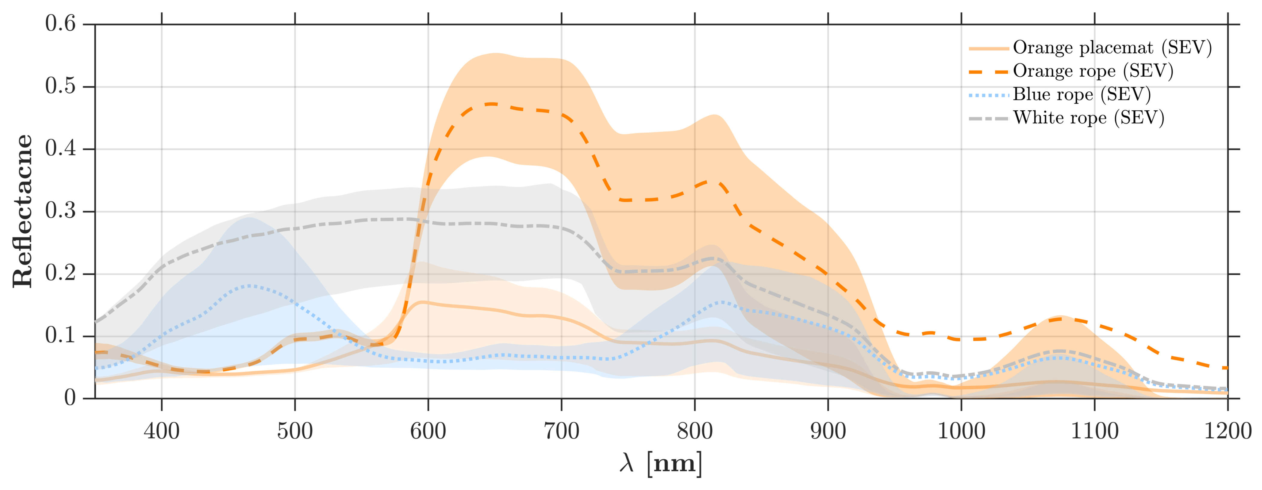
Figure 1. Examples of mean and 75% confidence bound of plastic litter spectra for orange placemat, orange rope, blue rope, and white rope in the SEV data.
Remotesensing 16 00172 g001
Figure 2. (a) The scaled spectrum of clear and turbid water at two different concentrations of suspended sediments collected by an ASD spectroradiometer. The mean (median) and 75% confidence bound of the plastic litter spectra in clear and turbid waters are shown with solid (dashed) lines and shaded areas for (b) SEV and (c) ASD data, where peak reflectance values are marked with arrows. Examples of plastic litter in the data set include (d) orange placemat, (e) unrolled blue polypropylene rope, and (f) unrolled white polyester rope [13].
Remotesensing 16 00172 g002
Figure 3. (ac) Reconstruction of the spectrum (solid black lines) of a dry orange placemat with different sparsities of k = 1 , 3 , 6 and the corresponding root mean squared error (RMSE). The position of important wavelengths (vertical red lines) corresponds to the wavelengths identified by apexes of the triangle basis functions (gray dashed lines) selected through solving Equation (1) as explained in Algorithm 1.
Remotesensing 16 00172 g003
Figure 4. The probability density function p Λ ( λ c ) of important wavelengths for wet plastics in clear (solid line) and turbid (dashed line) waters obtained from observations using (a) a Spectral Evolution (SEV) and (b) an ASD FieldSpec 4 spectroradiometer for 64 and 90 samples, respectively. The densities were obtained for k = 1 , , 5 , where the color bar represents the density of the points used in the kernel density estimation.
Remotesensing 16 00172 g004
Figure 5. The probability density functions p Λ ( λ c ) of important wavelengths for k = 1 , , 5 ; triangular basis functions obtained from 61 observed dry plastic spectra collected by the ASD FieldSpec 4 spectroradiometer.
Remotesensing 16 00172 g005
Figure 6. Central wavelengths associated with the modes of p Λ ( λ c ) for sparsities ranging from k = 1 to 15 using both SEV and ASD data of wet plastic samples. The uncertainty value of each mode is shown with blue bubble sizes determined based on the width of the pdf at 95% height of its modes [74]. For example, for k = 1 , the bubble is centered around 641 nm , with the uncertainty bound equal to 79 nm .
Remotesensing 16 00172 g006
Figure 7. (a) Correlation matrix of wet plastic spectral reflectance values within wavelengths 350–1200 nm using augmented SEV and ASD reflectance data. (b) The density peak clustering decision graph using the wet plastic spectral reflectance data. The top-10 wavelengths were selected based on the Euclidean distance from the origin reflectance values within wavelengths 350–1200 nm using augmented SEV and ASD reflectance data.
Remotesensing 16 00172 g007
Figure 8. Hierarchical clustering dendrogram with the color bar showing the range of distance cutoffs that lead to k c number of important wavelengths. For example, for k c = 3 , the cutoff range is between 0.24 to 0.38.
Remotesensing 16 00172 g008
Figure 9. Comparison of band selection results among sparse variable selection, hierarchical clustering, and density peak clustering (DPC) using reflectance data from wet plastic debris. The important wavelengths obtained by hierarchical clustering (blue circles), density peak clustering (bright red triangles), and the modes of p Λ ( λ c ) (red diamonds with dashed lines) for different sparsity values of k are shown. The green shaded areas depict the uncertainty values of Algorithm 1 defined as the width of p Λ ( λ c ) at 95% of the height of its modes. The numbers above the triangle markers indicate the rank of the wavelengths identified by the DPC algorithm. For example, the most important wavelength based on DPC is centered around 1095 nm .
Remotesensing 16 00172 g009
Figure 10. The reconstruction root mean square error (RMSE) using the variable selection method as a function of important wavebands k for wet plastics using both SEV and ASD data, with their 95 % confidence intervals shown by shaded areas. The red circle shows the reconstruction accuracy when the basis functions were centered around Sentinel-2 MSI wavelengths.
Remotesensing 16 00172 g010
Table 1. The number, type, and description of plastic litter samples collected by both ASD and SEV spectroradiometers [13].
ASDNumberDescriptionAge
Bottles7crushed, filled and emptyvirgin
PET Cups2flat and straightvirgin
Placemats *54different colors (orange, pink, blue, yellow)virgin
Ropes *68different colors (orange, blue, white), rolled, unrolled, aligned around framevirgin
Bags6different colors (white and black), wrinkled, aligned around framevirgin
Others2garden net and green foamvirgin
Weathered samples12gray cloth, waste rope, waste blue plastic bag, green rope waste, orange tube, transparent wrapping foil, pellets, extended polystyrene, energy drink container woodweathered
SEVNumberDescriptionAge
Placemats *19Orange placematvirgin
Ropes *45different colors (orange, blue, white)virgin
* Samples were placed at different depths.
Disclaimer/Publisher’s Note: The statements, opinions and data contained in all publications are solely those of the individual author(s) and contributor(s) and not of MDPI and/or the editor(s). MDPI and/or the editor(s) disclaim responsibility for any injury to people or property resulting from any ideas, methods, instructions or products referred to in the content.