Multi-Temporal and Time-Lag Responses of Terrestrial Net Ecosystem Productivity to Extreme Climate from 1981 to 2019 in China

Abstract

The escalating frequency and severity of extreme climate greatly impact the carbon dynamics of terrestrial ecosystems worldwide. To understand the multi-temporal response of net ecosystem productivity (NEP) to extreme climate, we investigated 11 temperature and precipitation extreme indices across different vegetation types in China. From 1981 to 2019, the results showed that NEP in China increased at a rate of 0.64 g·m⁻²·a⁻². Extreme climate demonstrated a significant warming trend and a non-significant moistening trend; specifically, maximum daily minimum temperature (TNx) exhibited a significant increase at a rate of 0.34 °C/10 a, while maximum 5-day precipitation (Rx5day) showed an insignificant increase at a rate of 1.78 mm/10 a. NEP was significantly impacted by extreme temperature at the annual, seasonal, and monthly scales, but moderately impacted by extreme precipitation. Specifically, extreme temperature had the most significant effect on grassland, with minimal influence on cropland. In contrast, extreme precipitation had the most significant effect on forest, with minimal impact on cropland. Moreover, the lagged time for extreme precipitation was longer than that for extreme temperature. Extreme precipitation exhibited a corresponding lagged time of at least 2 months (p < 0.01), while extreme temperature exhibited a lagged time of at least 1 month (p < 0.01). The maximum lag time observed was 4 months (p < 0.01). Our findings provide valuable insights into the multi-temporal response of NEP to extreme climate in China and inform sustainable development practices in the region.

1. Introduction

In recent decades, extreme climate have become increasingly common. The direct impact and potential threats are more diverse, more significant in magnitude, and more likely to occur than during average climate changes [1,2]. Global warming will further amplify the frequency, intensity, and geographic scope of these events, creating severe ecological consequences. Terrestrial ecosystems absorb approximately one-quarter of human-induced carbon dioxide emissions per year on average [3], playing a crucial role in decreasing the atmospheric carbon dioxide concentration and slowing global temperature increases [4]. In China, the land ecosystem is a critical part of the global carbon sink, accounting for 8–11% of the world’s total carbon storage [5,6]. Due to climate change, it exhibits significant regional disparities and annual variations, making it among the world’s most heavily affected areas due to extreme climate [7,8].

The response of the terrestrial ecosystem carbon cycle to extreme climate in mainland China exhibits a diverse and uncertain spatiotemporal pattern. Previous research has primarily focused on specific ecologically vulnerable or sensitive regions in China, such as the Chinese monsoon region [9], the Loess Plateau [10], the Qinghai–Tibet Plateau [11], the Weihe River Basin [12], and the agro-pastoral transitional zone [13]. However, a thorough and quantitative assessment of the spatiotemporal heterogeneity of the impact of different extreme climate factors on the carbon sink capacity of terrestrial ecosystems across the country is lacking. Differences in the ecological environments and vegetation coverage in various geographical regions lead to inconsistent patterns of the ecosystem’s response to extreme climates [14]. For instance, while extreme high temperatures prompt productivity in grassland ecosystems of the northwest Qinghai–Tibet Plateau, they hinder productivity in forest ecosystems of the hot and arid river valley region in Yunnan [15]. Additionally, multiple regions have noted increased vegetation productivity due to extreme precipitation [16,17,18], but the Loess Plateau did not experience significant effects on vegetation productivity concerning seasons or years [19]. Detailed information is necessary, considering the intricacies of carbon cycle responses to climate extremes and their interdependence with background ecosystem and climate conditions [20,21].

Similarly, the impact process of natural factors and the resulting changes happen at varying time scales and develop over time [22]. A single time scale analysis is insufficient to accurately demonstrate vegetation’s response mechanism to extreme climate changes [13]. It is necessary to investigate the differences in response to extreme climate on a monthly, seasonal, and annual scale for various vegetation types in mainland China. The carbon cycle in terrestrial ecosystems also shows a lagged impact of extreme climate, with longer-lasting effects than the direct influence of climate change [23]. Previous studies have indicated the time-lag range in vegetation’s response to extreme climate lasts from several months to more than a year. Liu et al. (2013) [17] and [24] found a time lag of 2–3 months between ecosystem indicators (NDVI and LAI) and extreme climate indices. In a precipitation control experiment on the semiarid grasslands of Inner Mongolia, China, the impact of extreme precipitation on ecosystem carbon absorption lasted up to two years [25]. Generally, the same vegetation type exhibits different time-lag effects due to various extreme climates, and differing vegetation types react differently to the same climate change [23]. Therefore, the time-lag effect is particularly important in understanding the ecological process of a terrestrial ecosystem responding to extreme climate.

In summary, in previous studies on the response of NEP in China to extreme climates, there is a relative lack of application of multiple methods to analyze the relationship between the two. The discussion is limited in terms of different time scales, including monthly, seasonal, and annual scales. And, further clarification is required concerning the lagged response behavior of different vegetation types to various extreme climates. To further explore the above issues, we took the mainland China region as a case study area, quantitatively described the spatiotemporal dynamics of carbon cycling in different terrestrial ecosystems from 1981 to 2019, detected the changing trends of extreme climate, and analyzed the response relationship between the ecosystem (net ecosystem productivity as the indicator) and various extreme climate indices in multi-temporal scales. This study aimed to clarify the following issues in mainland China: (1) What are the spatiotemporal characteristics of carbon cycling in terrestrial ecosystems? (2) What is the changing trend of extreme climate? (3) What are the responses of terrestrial net ecosystem productivity to extreme climate at different time scales?

2. Materials and Methods

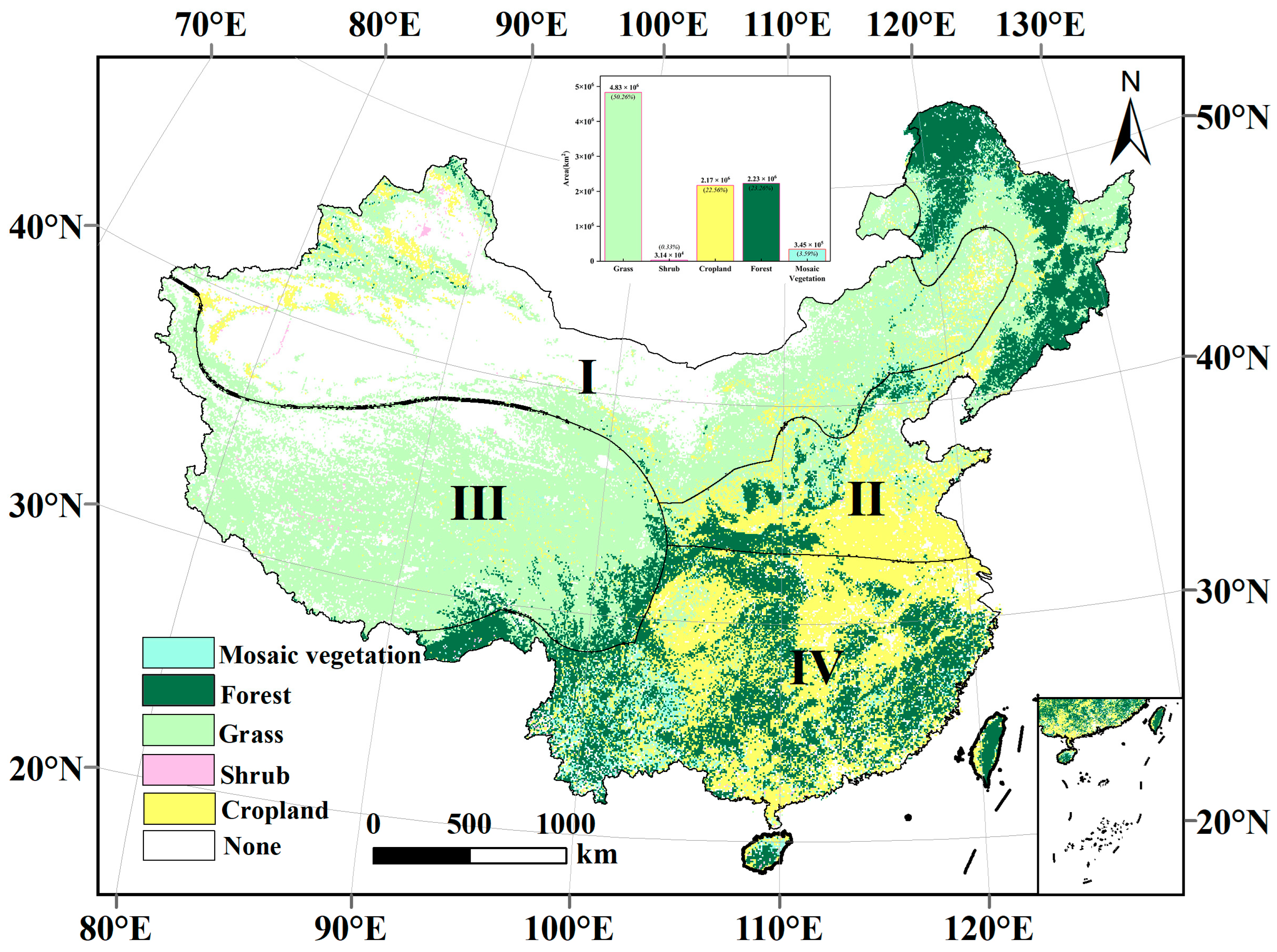
2.1. Study Area

China is primarily located in the subtropical zone of the northern hemisphere and mid-latitude region, with a geographic location between 3°51′ and 53°33′N and 73°33′ and 135°05′E along the east of Asia and west coast of the Pacific Ocean. Due to the lack of meteorological data, the Taiwan Province, Hong Kong, and Macao Special Administrative Regions were excluded from the study area. The study area can be categorized into four regions based on climatic conditions: the temperate continental zone, the temperate monsoon zone, the high–cold Tibetan Plateau, and the subtropical–tropical monsoon zone [26]. From 1981 to 2019, the average annual precipitation varied across different climatic zones as follows: the temperate continental zone received 269 mm, the temperate monsoon zone experienced 585 mm, the high–cold Tibetan Plateau received 382 mm, and the subtropical–tropical and tropical monsoon zones witnessed 1320 mm of rainfall per year.

2.2. Material

The Boreal Ecosystem Productivity Simulator (BEPS), which is driven by remote sensing, is used to generate the carbon flux of terrestrial ecosystems. Comprising various modules, including energy transfer, carbon and nitrogen cycles, water cycle, and physiological regulation, the model’s carbon and nitrogen cycle module involves plant photosynthesis, respiration, carbon allocation, litterfall, soil organic carbon and nitrogen decomposition [27]. The canopy is divided into sunlit and shaded leaves by BEPS, enabling the simulation of their total gross primary productivity (GPP) and transpiration separately; the net primary productivity (NPP) is calculated as the difference between GPP and autotrophic respiration. In accordance with vegetation type, the NPP allocation ratio and conversion rate are utilized to update four vegetative carbon pools daily. The decomposition rate of nine litter and soil carbon pools is determined using simulated soil temperature and humidity. Heterotrophic respiration (Rh) is calculated as the total proportion of CO₂ released to the atmosphere during litter and soil carbon pool decomposition, and the net ecosystem productivity (NEP) is calculated as the difference between NPP and Rh.

To accurately simulate sunlit and shaded leaf area and GPP, the LAI and clumping index are both necessary. LAI serves as the foundation for simulating the carbon flux. The GLOBMAP LAI data product was created by integrating MODIS reflectance data and AVHRR GIMMS NDVI data spanning 1981 to 2019. From 1981 to 1999, the temporal resolution was 15 or 16 days, while from 2000 to 2019, it was 8 days. During the simulation, the LAI values for 16-day and 8-day intervals were interpolated to obtain daily values. The clumping index (CI) characterizes the three-dimensional canopy structure. The daily CI over a large area can be estimated from MODIS BRDF remote sensing data using an empirical relationship with the normalized difference between hotspots and dark spots [28]. The initial values for the four vegetation carbon pools and the nine litter and soil organic carbon pools are particularly critical. Assuming that the ecosystem was in carbon balance (NEP equals zero) in 1901, the BEPS model is driven by the average LAI from 1981 to 1985 (which exhibits seasonal variation), average climate data from 1901 to 1910, and CO₂ concentration and nitrogen deposition data from 1901 to initialize the soil carbon pools, allowing each carbon pool to reach a near-steady state. Subsequently, for the period of 1901–1980, the model is driven by the average LAI from 1981 to 1985 (with seasonal variation), time-varying climate, CO₂ concentration, and nitrogen deposition data. For the period of 1981–2019, the model is driven by temporally varying LAI, climate, CO₂ concentration, and nitrogen deposition data.

The BEPS model, applied widely in global regions, simulates terrestrial ecosystem carbon flux and evaluates the effects of various driving factors [27,29]. This model introduces advanced radiative transfer theory and fine photosynthesis. With the module, multi-source data are integrated as the input of the model, and the carbon water process module is coupled; the time resolution of the model is daily, which can be better simulated and larger NEP at spatial scales. He et al. (2021) [30] validated the BEPS model using eddy-covariance flux data and found it to be a reliable means of simulating the NEP of China’s terrestrial ecosystems. Here, we present NEP simulation results obtained daily during the period of 1981–2019, which was generated by Chen et al. (2019) [27] and can be obtained from National Ecosystem Science Data Center, National Science and Technology Infrastructure of China (http://www.nesdc.org.cn/, accessed on 20 December 2023), with a spatial resolution of 0.072727° × 0.072727°.

Long-term site-based meteorological data, including rainfall, high temperature, and low temperature, were obtained from China Meteorological Data Network (http://data.cma.cn/, accessed on 20 December 2023).

We used the European Space Agency Climate Change Initiative Land Cover dataset (CCI-LC) (http://maps.elie.ucl.ac.be/CCI/viewer/index.html, accessed on 20 December 2023) to collect the land cover data (Figure 1). The CCI-LC dataset provides a land cover map with a spatial resolution of 300 m and divides the surface cover into 37 categories based on the Land Cover Classification System (LCCS) developed by the Food and Agriculture Organization of the United Nations [31,32]. We resampled it to 8 km to align with the spatial resolution of the NEP data and to facilitate subsequent correlation analysis. Additionally, the vegetation was merged and classified into five categories, including shrub, forest, grassland, cropland, and mosaic vegetation (mixed needle and broad leaf tree cover), based on the International Geosphere–Biosphere Programme (IGBP) classification scheme and the actual vegetation distribution in China.

2.3. Methods

2.3.1. Selection of Climate Extreme Indices

According to meteorological data obtained from Chinese meteorological stations, 11 extreme climate indices were computed using the RClimDex 1.9.2 software (https://github.com/ECCC-CDAS/RClimDex, accessed on 20 December 2023), as illustrated in

Table 1. Climate extreme indices of temperature and precipitation.

Index	Definition	Unit
Temperature
TNn	Minimum value of daily minimum temperature	°C
TNx	Maximum value of daily minimum temperature	°C
TXn	Minimum value of daily maximum temperature	°C
TXx	Maximum value of daily maximum temperature	°C
Tn10p	Count of days where TN < 10th percentile	days
Tn90p	Count of days where TN > 90th percentile	days
Tx10p	Count of days where TX < 10th percentile	days
Tx90p	Count of days where TX > 90th percentile	days
DTR	Mean value of difference between TX (daily maximum temperature) and TN (daily minimum temperature)	°C
Precipitation
Rx1day	Maximum precipitation amount in one-day period	mm
Rx5day	Maximum total precipitation amount in consecutive five-day period	mm

[1,33]. The selection of these indices was guided by the research objectives and the consideration of multiple climatic regions. The chosen indices offer a comprehensive representation of possible extreme climate conditions on a monthly, seasonal, and yearly basis. They are effective in identifying frequent occurrences of extreme weather events as opposed to rare occurrences that happen once in a decade [34]. Furthermore, these indices are simple to understand and have wide applicability, as they have been used in previous studies.

2.3.2. The Linear Regression Method

The temporal trends of ecosystem productivity and extreme climate indices were characterized using the linear regression method. The slope of the linear regression based on least squares fitting represents the annual change rate of NEP and extreme climate indices. A positive value indicates an increasing trend, while a negative value indicates a decreasing trend. The linear equation is presented in Equation (1):

$$\mathrm{y}=\mathrm{b}\ast \mathrm{x}+\mathrm{a}$$

(1)

The equation considers one of the dependent variable time series datasets to be $\mathrm{y}$, with $\mathrm{x}$ representing the time series from 1981 to 2019. The variables a and b denote the intercept and slope of the dependent variable, respectively. The analysis utilizes a significance level of 0.05.

2.3.3. Partial Correlation between NEP and Extreme Climate Indices

The partial correlation coefficient serves as a measure of the relationship among multiple factors [2]. In this study’s multi-factor system, the partial correlation method was utilized to explore the correlation between individual factors, while controlling for the influence of other factors. The formula for calculating the partial correlation is:

$${\mathrm{R}}_{\mathrm{x}\mathrm{y},\mathrm{a},\mathrm{b}}=\frac{{\mathrm{R}}_{\mathrm{x}\mathrm{y},\mathrm{a}}-{\mathrm{R}}_{\mathrm{x}\mathrm{b},\mathrm{a}}{\mathrm{R}}_{\mathrm{y}\mathrm{b},\mathrm{a}}}{\sqrt{(1-{\mathrm{R}}_{\mathrm{x}\mathrm{b},\mathrm{a}}^2)(1-{\mathrm{R}}_{\mathrm{y}\mathrm{b},\mathrm{a}}^2)}}$$

(2)

The equation represents the partial correlation coefficient of different time scales of variables $\mathrm{x}$ and $\mathrm{y}$, ranging from [−1.0, 1.0], where a higher value implies a more robust correlation between the variables. ${\mathrm{R}}_{\mathrm{x}\mathrm{y},\mathrm{a}}$, ${\mathrm{R}}_{\mathrm{x}\mathrm{b},\mathrm{a}}$, and ${\mathrm{R}}_{\mathrm{y}\mathrm{b},\mathrm{a}}$ denote the partial correlation coefficients between variables $\mathrm{x}$ and $\mathrm{y}$, variables $\mathrm{x}$ and $\mathrm{b}$, and variables $\mathrm{y}$ and $\mathrm{b}$, respectively, after removing the influence of variable $\mathrm{a}$. The recent forty year time series for each vegetation type and extreme climate indices were analyzed using MATLAB R2022b (https://www.mathworks.com/, accessed on 20 December 2023) [35].

2.3.4. Lagged Response of NEP to Extreme Climate Indices

Previous studies have reported that vegetation’s response to climate usually lags by less than a quarter of a month at a monthly scale [36,37]. Hence, this research assumes a lag time of 0–4 months. Equation (3) presents the association between NEP and extreme climate indicators:

$$\mathrm{N}\mathrm{E}\mathrm{P}={\mathrm{k}}_{\mathrm{i}}\ast \mathrm{f}\mathrm{a}\mathrm{c}\mathrm{t}\mathrm{o}\mathrm{r}+\mathrm{b}$$

(3)

The variable ${\mathrm{k}}_{\mathrm{i}}$ represents the regression coefficient of a time lag of $\mathrm{i}$ months, where $\mathrm{i}$ ranges from 0 to 4 (0 indicates no lag effect, and 1–4 denote lags of 1–4 months, respectively). The NEP time series spans from 1981 to 2019, while the factor comprises the time series of each extreme climate index with a time lag of $\mathrm{i}$. Based on each extreme climate factor, the lag month with the highest R² value determines the optimal lag time for the NEP response to the extreme climate factor. The latest time for R² to manifest as significant was defined as the longest response time. If the NEP exhibits significant performance in the first, second, and third lag months, but not in the fourth lag month, we defined a lag time as three months.

3. Results

3.1. NEP Dynamics during 1981–2019

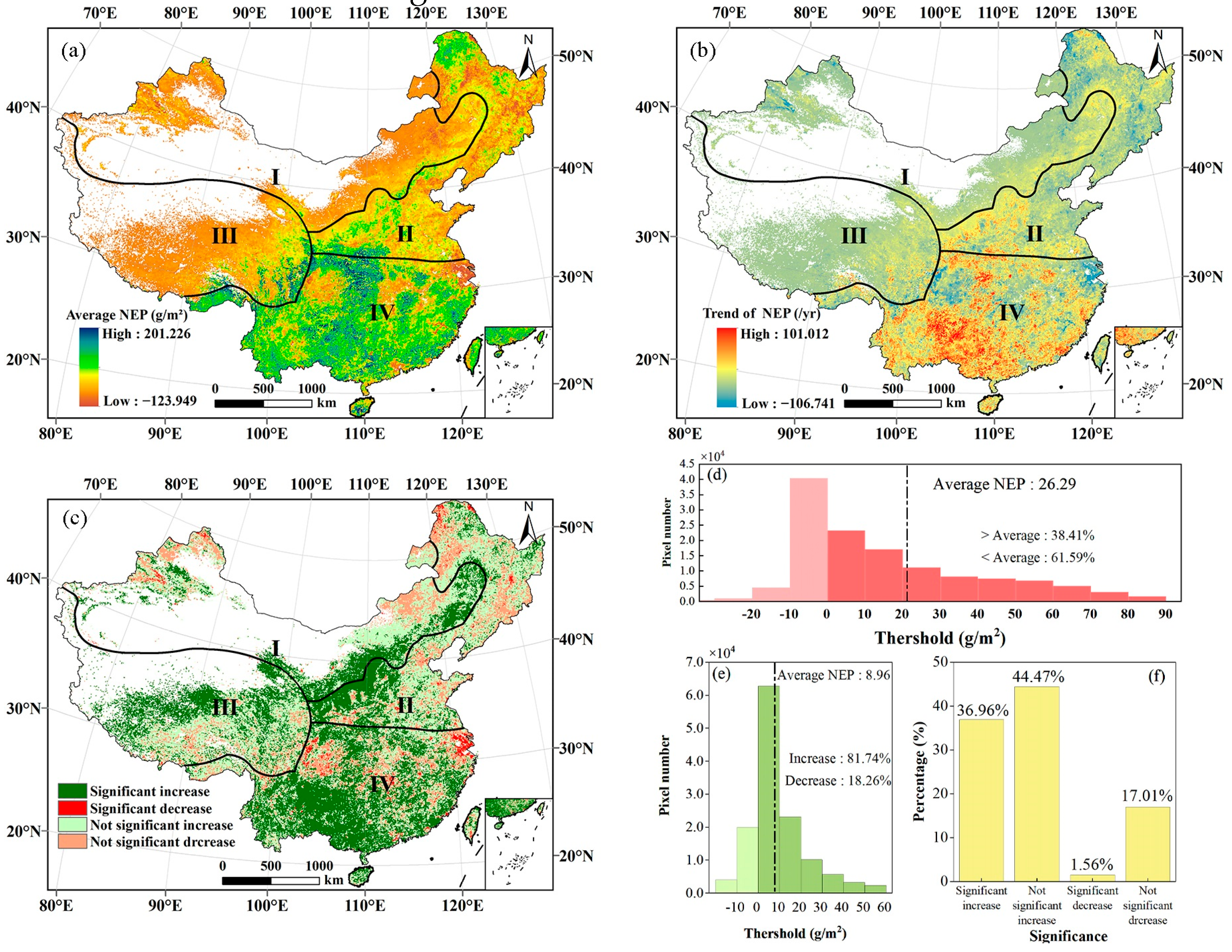
3.1.1. Spatiotemporal Dynamics of China’s NEP from 1981 to 2019

In mainland China, the mean NEP has increased by a rate of 0.64 g·m⁻²·a⁻² over the past four decades, as illustrated in Figure 2.

During the study period (1981–2019), the NEP values were comparatively low in the grasslands of the western and northern regions, whereas they were high in the central to southern regions, as well as in some areas of northeastern China, which were primarily covered in forests and mosaic vegetation (Figure 1). The study identified that regions with NEP values greater than the overall average (26.29 g·m⁻²·a⁻²) accounted for 38.41% of the entire study area (Figure 3e). Of the total change in NEP, 81.74% showed an increase while 18.26% showed a decrease (Figure 3e). Furthermore, significant increases and decreases were observed in 36.96% and 1.56% of the country, respectively (Figure 3f). Areas with significant decreases in NEP were mostly concentrated in the eastern coastal regions where forests contributed to a high overall NEP value.

3.1.2. Spatiotemporal Variations in Vegetation NEP from 1981 to 2019

Among the different vegetation types, mosaic vegetation witnessed the highest annual increase in NEP (1.92 g·m⁻²·a⁻²; p < 0.001), followed by forest land (1.18 g·m⁻²·a⁻²; p < 0.001), cropland (0.72 g·m⁻²·a⁻²; p < 0.001), shrub (0.59 g·m⁻²·a⁻²; p = 0.18), and grassland (0.37 g·m⁻²·a⁻²; p < 0.001). Forest land exhibited the highest NEP values, ranging from −4.46 g·m⁻²·a⁻² to 109.17 g·m⁻²·a⁻², while shrub showed the lowest NEP values, ranging from −46.7 g·m⁻²·a⁻² to 84.38 g·m⁻²·a⁻² (Figure 4).

From 1981 to 2019, the proportions of carbon sources (average NEP < 0) in the region were as follows: grass (2.23%), cropland (1.00%), forest (0.66%), mosaic vegetation (0.01%), and almost negligible in shrub (

Table 2. Proportions of area in NEP among five different vegetation types from 1981 to 2019 (%).

Average NEP (g·m−2)	Grass	Shrub	Cropland	Forest	Mosaic Vegetation	Total
<−20	0.13	0.00	0.06	0.06	0.01	0.26
−20–−10	0.36	0.00	0.19	0.11	0.02	0.68
−10–0	1.73	0.00	0.75	0.49	0.09	3.06
0–10	22.78	0.10	3.68	1.71	0.47	28.75
10–20	9.41	0.01	5.72	2.47	0.64	18.25
20–30	5.35	0.01	4.68	2.93	0.60	13.58
30–40	2.48	0.01	2.92	3.02	0.47	8.89
40–50	1.02	0.01	1.84	3.20	0.42	6.49
50–60	0.52	0.02	1.54	3.34	0.45	5.86
60–70	0.29	0.03	1.41	3.25	0.41	5.39
70–80	0.17	0.02	1.04	2.46	0.25	3.93
80–90	0.09	0.01	0.62	1.59	0.13	2.44
>90	0.11	0.01	0.54	1.67	0.11	2.43
Trend of NEP (g·m−2·a−2)	Grass	Shrub	Cropland	Forest	Mosaic Vegetation	Total
<−20	0.11	0.00	0.20	0.25	0.01	0.56
−20–−10	0.32	0.00	0.59	1.08	0.03	2.03
−10–0	5.31	0.03	2.78	4.14	0.26	12.51
0–10	37.53	0.22	8.52	6.84	1.01	54.11
10–20	5.48	0.04	4.96	4.66	0.83	15.98
20–30	1.06	0.02	2.43	2.94	0.57	7.03
30–40	0.31	0.01	1.44	1.75	0.38	3.89
40–50	0.09	0.01	0.92	0.96	0.27	2.25
50–60	0.03	0.01	0.45	0.39	0.15	1.04
>60	0.02	0.00	0.25	0.23	0.09	0.60
Significance of Trend	Grass	Shrub	Cropland	Forest	Mosaic Vegetation	Total
Significant increase	14.79	0.10	11.10	8.98	2.40	37.36
Significant decrease	22.29	0.10	9.73	11.30	1.34	44.76
Not significant increase	0.25	0.00	0.59	0.42	0.02	1.28
Not significant decrease	6.79	0.03	3.71	5.75	0.32	16.60

). Similarly, the proportions of carbon sinks (average NEP > 0) in the region were as follows: grass (42.22%), forest (25.63%), cropland (23.98%), mosaic vegetation (3.94%), and shrub (0.23%). Grassland demonstrated the most significant decreasing trend in NEP (5.75%) and shrub (0.03%) showed the least variation. Moreover, grassland exhibited the most significant increasing trend in NEP (44.53%). Only 1.28% of the total area was covered by regions experiencing a significantly decreasing trend in NEP, with cropland (0.59%) making the greatest contribution.

3.2. Annual Variation of Extreme Climate Indices during 1981–2019

Several temperature indices indicated a significant warming trend in mainland China. Extreme heat indices strengthened significantly, while the duration and intensity of extreme cold decreased considerably. Both warm nights (Tn90p) and warm days (Tx90p) increased significantly at rates of 4.39 days/10a (p < 0.05) and 3.62 days/10a (p < 0.05), respectively. The cold nights (Tn10p) decreased significantly at a rate of 0.45 days/10a (p < 0.05), whereas the change in cold days (Tx10p) was not significant. TXx and TNx values significantly increased at rates of 0.37 and 0.35 °C/10 a (p < 0.05), respectively. Conversely, TXn and TNn showed a non-significant upward trend (p > 0.05). DTR decreased at a rate of 0.04 °C/10 a (p = 0.12). Meanwhile, extreme precipitation events in China (Rx1day and Rx5day) displayed a non-significant upward trend from 1981 to 2019, with rates of change of 1.33 and 1.78 mm/10 a (p > 0.05) (Figure 5).

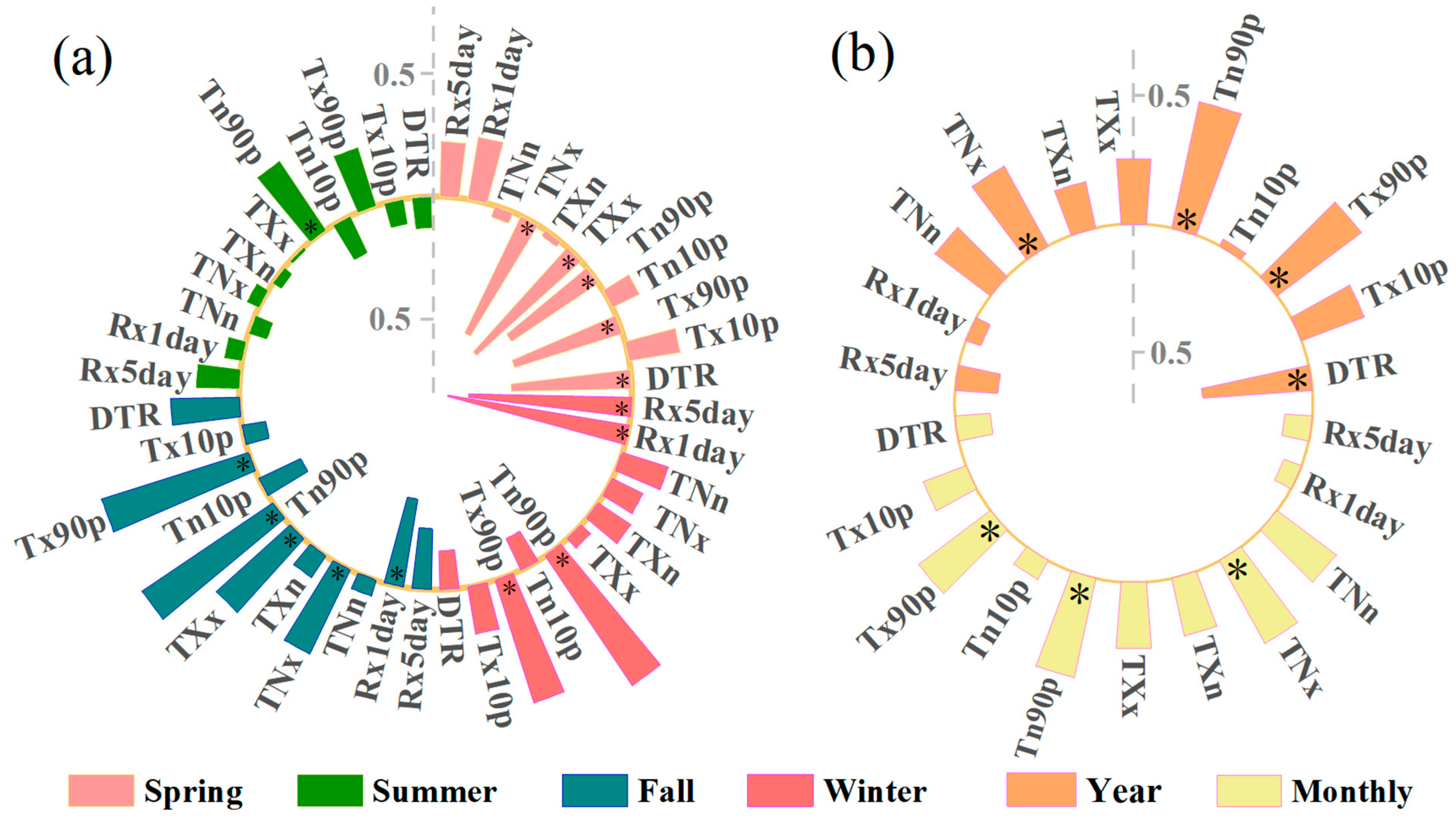
3.3. The Response of NEP to Extreme Climate Indices at Annual, Seasonal, and Monthly Time Scales

In mainland China, the temperature indices indicated a significant warming trend. NEP showed a strong positive correlation with extreme temperature at annual, seasonal, and monthly scales. The correlation with extreme precipitation was relatively weaker. TNx, Tn90p, and Tx90p were significantly and positively correlated with NEP annually (p < 0.01). Among them, Tn90p had the strongest correlation coefficient of 0.50, followed by Tx90p (0.41) and TNx (0.36). DTR also showed a significant positive correlation with NEP (0.43, p < 0.01). Extreme precipitation had an insignificant impact on NEP. At the seasonal scale, there was a significant correlation between NEP and extreme climate, with variations from spring to winter. In spring, extreme temperatures were negatively correlated with NEP (p < 0.05). However, in autumn, Tn90p and Tx90p had a significant positive impact on NEP (p < 0.05), while in winter, only Tn90p and Tx90p showed a significant positive impact. Regarding extreme precipitation, the impact of Rx1day and Rx5day on NEP increased from spring to winter, with positive correlations in spring and summer, and negative correlations in autumn and winter (significant in winter, p < 0.05). Therefore, extreme temperature primarily influences NEP at the seasonal scale in mainland China. At the monthly scale, NEP had a significant correlation with Tx90p, Tn90p, and TNx, but insignificant correlations with DTR and other extreme temperature indices. NEP also showed a weak and insignificant correlation with Rx1day and Rx5day. Overall, extreme temperatures are the primary influencing factor on monthly scale NEP in mainland China (Figure 6).

3.4. Seasonal Response of NEP to Extreme Climate Indices across Different Vegetation

NEP and extreme temperatures had varying relationships across different vegetation types. Correlations between NEP and extreme precipitation were not significant. In grassland ecosystems, extreme temperatures in spring and summer (TNn, TXn, Tn10p, Tx90p) negatively impacted NEP, but positively impacted it in autumn. TNx had a positive impact in autumn and winter. For shrub ecosystems, TNx had a positive impact in all seasons, and TXn had a positive impact in autumn, while other temperature indices had weak or insignificant correlations throughout the year. In cropland ecosystems, TNn, TXn, Tn10p, and Tx90p negatively impacted NEP in spring, while TNx and TXx had a positive impact in autumn. In winter, Tn10p had a negative impact, but other extreme temperature indices had weak or insignificant effects. In forest ecosystems, TNx had a positive impact in spring, autumn, and winter, while Tx10p and Tn10p had negative impacts in spring and autumn. TXx had a positive impact in autumn, and Tx90p had a negative impact in spring and autumn. In mosaic vegetation ecosystems, TNx, TNn, Tn90p, Tx90p, and Tx10p had negative impacts in spring but positive impacts in autumn. TXn had a negative impact in spring but positive impacts in the other three seasons. DTR had the most significant effect on NEP in shrub ecosystems in winter and in forest ecosystems in spring. Grassland ecosystems were the most affected by extreme temperature indices, followed by forest, mosaic vegetation, and shrub ecosystems, while cropland ecosystems showed the smallest impact.

The results showed that grassland had a positive correlation with extreme precipitation only in summer, shrub showed a positive correlation in spring, and forest showed a positive correlation in winter. Mosaic vegetation and cropland did not have a significant correlation with extreme precipitation throughout the seasons. Forest was the most impacted by extreme precipitation, followed by shrub, grassland, and mosaic vegetation, while croplands had the smallest impact. However, the overall correlations between NEP and extreme precipitation indices for different vegetation types were small and insignificant.

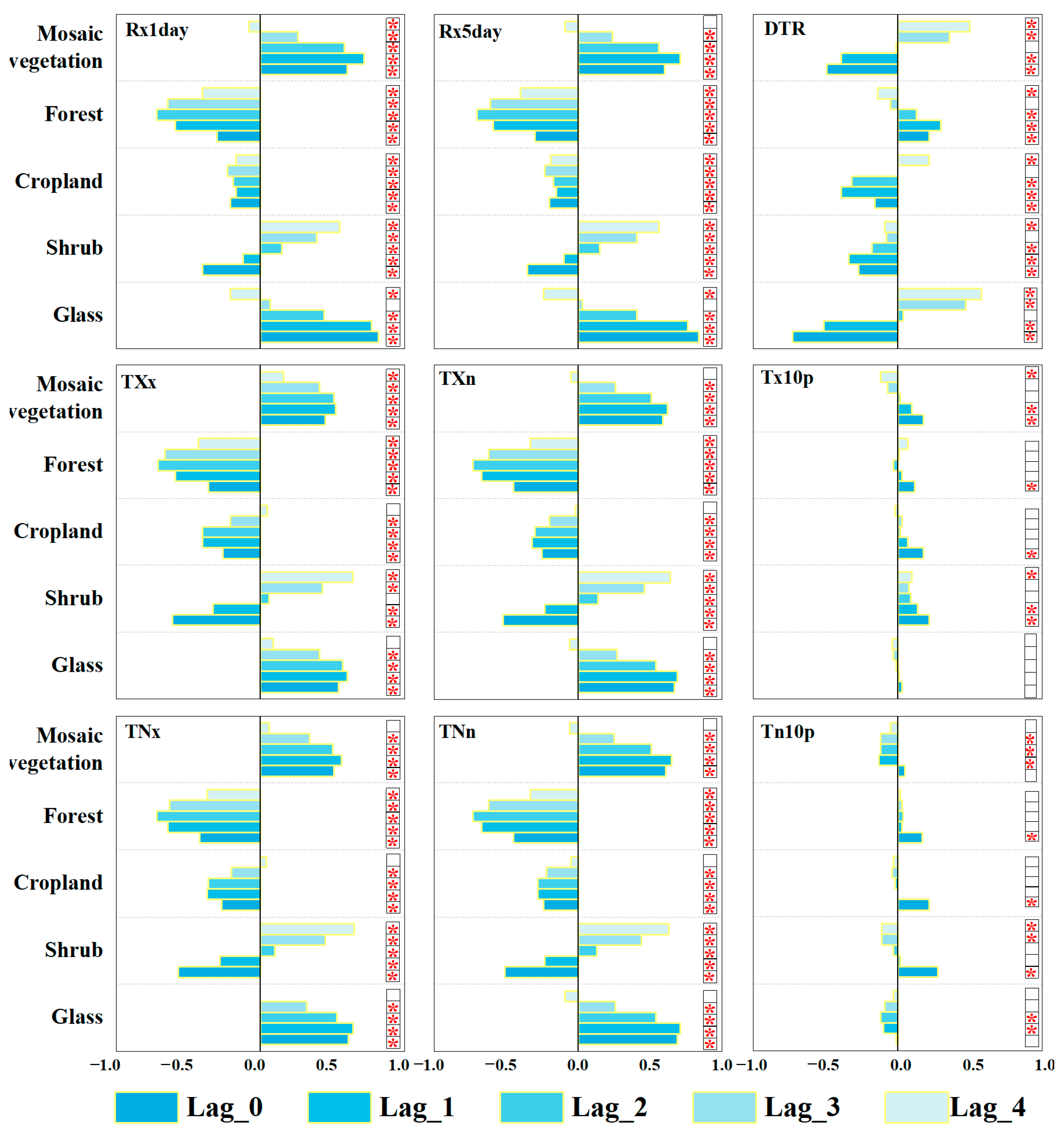
3.5. Time-Lag Response of NEP to Extreme Climate Indices

The time-lag response of NEP to extreme climate indices from 0 to 4 months is shown in Figure 7. Different vegetation types had significantly different delayed effects from the same extreme climate factor, and the time-lag effects of the same vegetation type from different extreme climate indices also had significant differences. The delayed response of vegetation to extreme precipitation (Rx1day, Rx5day) was longer than that to extreme temperature (TNn, TNx, TXn, and TXx), with a lag time of at least 2 months (p < 0.01) and at least 1 month (p < 0.01), respectively, and up to 4 months (p < 0.01). The lagged response of vegetation is reflected differently: with respect to extreme temperature, except for the one-month response of shrubs to TXx (p < 0.01), the responses of the remaining four vegetation types to TNn, TNx, TXn, and TXx all showed a lag of at least 3 months (p < 0.01). In particular, in forests, the lag time with respect to the extreme temperature index reached 4 months (p < 0.01), and the correlation coefficient was higher in the third month of lag compared to other vegetation types.

With regard to extreme precipitation, the lag time of grassland was 2 months (p < 0.01), and that of mosaic vegetation was at least 3 months (p < 0.01), while the lagging response of shrubs, cropland, and forests was 4 months (p < 0.01). The lag-time of the effect of diurnal temperature range (DTR) on different vegetation types was at least 1 month (p < 0.01). The lagged effect of cold days and nights (Tn10p, Tx10p) on NEP impact based on different vegetation types was insignificant.

4. Discussion

4.1. Dynamic of NEP and Extreme Climate Indices in Mainland China

There were substantial spatial variations in the changes in NEP in mainland China during the period from 1981 to 2019 (Figure 3). The significant increase in NEP predominantly occurred in China’s tropical and subtropical monsoon climate regions, which is primarily attributed to the regional warming and humid environment that extends the growing season, thereby promoting plant productivity and carbon fixation [38,39]. On the contrary, the NEP in the eastern coastal areas, particularly in the Yangtze River Delta region, exhibited a significant decrease. This decline was primarily due to rapid human activities, such as urbanization and industrialization that resulted in large-scale deforestation, which directly decreases carbon fixation through reducing vegetation coverage [40]. Moreover, the increase in anthropogenic emissions, including fossil fuel combustion and cement production, has led to a rise in atmospheric carbon dioxide concentration, significantly amplifying carbon emissions in the ecosystems [41].

The analysis of the extreme climate index indicated that extreme temperature has generally increased in mainland China, while extreme precipitation has not changed significantly over the years, as depicted in Figure 5. This outcome supports the findings of other research studies [8,42,43]. Comparable patterns have been found in various regions of China, such as the agro-pastoral zone in North China [13], eastern coastal area [44], the Yangtze River Basin [45], and the Qinghai–Tibet Plateau region [46]. It is important to note that the warming demonstrates an asymmetrical feature, where the indices linked to cold temperatures (Tn10p, Tn90p, TNn, TNx) have rapidly increased compared to those related to warm temperature (Tx10p, Tx90p, TXn, TXx) (Figure 5). The decrease in the national DTR over the last four decades has also demonstrated that the warming at night is more prominent than in the day. This phenomenon is universal [47], and it is mainly due to the alteration of the worldwide cloud cover which reduces temperatures during the day by attenuating shortwave sunlight and warms up the earth’s surface at night by reflecting longwave radiation back [48,49]. The research indicates that when there is an average global increase in daily cloud cover, warming in both the minimum night temperature and maximum daytime temperature occurs. However, the temperature rise at night is typically more significant than during the day, by more than 0.25 °C, and occupies an area 2.07 times larger than the latter (covering 36.7% and 17.7% of land cover, respectively) [49]. Enhanced soil moisture enhances soil–plant transpiration and impedes the daytime maximum temperature [50], whereas increased precipitation triggers the formation of more clouds which increases soil humidity, enhancing the aforementioned physical and ecological processes [51]. Additionally, local human activities, such as an increase in low-reflectivity surface coverings like artificial surfaces, increase the daytime heat absorption and nighttime heat release [52]. The combined effects of these processes result in the asymmetrical warming observed in mainland China.

4.2. Multi-Temporal Response Mechanisms of Net Ecosystem Productivity to Extreme Climate in Different Vegetation

Varying temporal and spatial scales in terms of grain size and extent significantly affect the results of spatial analyses of landscape patterns [53]. The relationship between vegetation types and climate factors varies across different time scales. A comprehensive analysis that considers only a single time scale makes it challenging to accurately assess how vegetation responds to climate change [13,54]. For instance, in arid and semiarid ecosystems, the response of vegetation to rainfall events shows time-scale dependence [55,56]. In their investigation of vegetation and precipitation responses in the Sahel–Sudano–Guinean region, Zhou et al. (2021) [56] demonstrated that the significance of vegetation response to rainfall is limited to certain localized areas of the Sahel at both interannual and intra-annual scales. In other regions, the response is primarily significant on a yearly or semi-annual (6-month) basis. In the annual assessment, the sustained rise in extreme high temperatures (TXx and TXn) stimulates an enhancement in NEP. This is attributed to the fact that high temperatures accelerate spring phenology, facilitating vegetation growth, and intensify vegetation transpiration during summer [57,58]. Nevertheless, the productivity gain from the former aspect generally surpasses the respiration increase from the latter, ultimately leading to an overall augmentation in the ecosystem’s carbon absorption throughout the year.

Figure 6 shows that the correlation and significance of NEP with extreme precipitation and temperature follows a trend of monthly > seasonal > annual scale. The observed trend can be attributed to two main factors. Firstly, longer time scales capture the cumulative impacts of long-term changes in the climate, whereas extreme climate produce rapid but relatively short-lived responses in NEP. Consequently, vegetation undergoes further recovery or regeneration [59], leading to a response that is difficult to detect over longer periods. Secondly, longer time scales are unable to discern the impact of multiple external factors like human activities (e.g., urbanization, irrigation, farming practices) and natural phenomena (e.g., solar radiation, landslides), which induce significant changes in ecosystem carbon cycling over shorter time periods [60].

4.3. Seasonal Response of Net Ecosystem Productivity to Extreme Climate in Different Vegetation

In the spring and summer, the NEP of grassland was significantly negatively correlated with warm indices (Tx90p) and TXn (

Table 3. Correlation between NEP of different vegetation and extreme climate indices on a seasonal scale. Note: * indicates that the p value is less than 0.05.

Spring	Grass	Shrub	Cropland	Forest	Mosaic Vegetation	Summer	Grass	Shrub	Cropland	Forest	Mosaic Vegetation
DTR	−0.27	−0.51 *	−0.39 *	−0.51 *	−0.43 *	DTR	0.02	−0.11	−0.36 *	−0.23	−0.12
TNx	−0.01	0.41 *	0.16	0.39 *	0.12	TNx	0.08	0.34 *	0.26	0.25	0.27
TNn	−0.63 *	−0.26	−0.47 *	−0.25	−0.54 *	TNn	−0.67 *	0.21	−0.04	0.05	0.19
TXx	0.00	0.27	0.07	0.23	0.02	TXx	0.38 *	0.25	0.13	0.12	0.22
TXn	−0.65 *	−0.08	−0.45 *	−0.21	−0.50 *	TXn	−0.67 *	0.20	0.13	0.21	0.33 *
Tn10p	−0.59 *	−0.39 *	−0.53 *	−0.48 *	−0.62 *	Tn10p	−0.49 *	0.26	−0.13	−0.08	0.13
Tx10p	−0.20	−0.17	−0.03	−0.05	0.03	Tx10p	−0.58 *	−0.03	0.01	0.05	−0.05
Tx90p	−0.60 *	−0.31	−0.49 *	−0.46 *	−0.63 *	Tx90p	−0.62 *	0.27	−0.17	−0.09	0.11
Tn90p	−0.25	0.04	−0.06	0.04	−0.03	Tn90p	−0.57 *	0.00	0.03	0.10	−0.02
Rx1day	0.10	0.47 *	0.17	0.32	0.21	Rx1day	0.59 *	−0.14	−0.07	−0.10	−0.14
Rx5day	0.07	0.46 *	0.15	0.31	0.26	Rx5day	0.63 *	−0.14	−0.24	−0.28	−0.26
Fall	Grass	Shrub	Cropland	Forest	Mosaic vegetation	Winter	Grass	Shrub	Cropland	Forest	Mosaic vegetation
DTR	−0.27	−0.32	−0.18	0.08	−0.04	DTR	−0.27	−0.65 *	−0.23	−0.40 *	−0.37 *
TNx	0.46 *	0.54 *	0.63 *	0.65 *	0.47 *	TNx	0.34 *	0.55 *	0.18	0.35 *	0.17
TNn	0.46 *	0.32	0.21	−0.32	0.50 *	TNn	0.20	−0.09	−0.06	0.27	0.34 *
TXx	0.12	0.12	0.42 *	0.74 *	0.12	TXx	0.30	0.19	0.09	0.01	−0.05
TXn	0.57 *	0.35 *	0.18	−0.45 *	0.49 *	TXn	0.22	0.16	0.03	0.29	0.44 *
Tn10p	0.23	0.20	0.19	−0.26	0.41 *	Tn10p	−0.10	−0.20	−0.42 *	−0.10	0.02
Tx10p	0.18	−0.07	−0.27	−0.56 *	0.18	Tx10p	−0.13	−0.34 *	0.10	0.08	0.24
Tx90p	0.31	0.18	0.13	−0.49 *	0.36 *	Tx90p	−0.12	−0.04	−0.30	−0.08	0.14
Tn90p	0.35 *	0.20	0.13	−0.42 *	0.39 *	Tn90p	−0.10	−0.15	0.03	0.12	0.23
Rx1day	−0.01	−0.05	−0.10	0.26	0.27	Rx1day	−0.17	0.31	0.22	0.37 *	0.14
Rx5day	−0.04	−0.06	−0.29	0.12	0.17	Rx5day	−0.27	0.28	0.11	0.34	0.08

). Extreme heat impacts land ecosystem NEP through increased plant and soil water evaporation and stomata closure due to a higher saturated water vapor pressure gradient, reducing the CO₂ supply and suppressing photosynthesis [61,62]. Prolonged extreme heat can also scorch leaves, damage plant photosynthetic machinery, and reduce productivity, which can even lead to plant death [60]. This also ultimately leads to a decrease in soil microbial activity and the total soil carbon pool. Based on the aforementioned impact mechanism, a meta-analysis of 79 global extreme climates (including 656 comparative observation experiments) showed that extreme heat significantly inhibits vegetation productivity and primarily reduces grassland ecosystem productivity, with an average decrease of 19.6% in GEP [62]. It was noticed that the extreme high temperatures faced by grassland ecosystems in the study area may not have fully reached the threshold for temperature responses in summer [63]. Therefore, as regional extreme maximum temperatures continue to rise until the reach a limiting point, they still exhibit a promotional effect on grassland NEP. However, this positive effect is relatively small and generally weak in the correlation. In the autumn, grassland along with warm indices (Tn90p) and TXn became significantly positively correlated because the retention of high temperatures briefly before the season delays chlorophyll degradation and leaf aging, slowing the decline in vegetation productivity and maintaining the ecosystem’s carbon sequestration capacity [64]. Hence, the response of grassland NEP to extreme high temperatures is modulated by the thermal adaptation of the ecosystem. During the spring and summer seasons, plants are in their active growth phase and exhibit heightened sensitivity to temperature fluctuations, thereby rendering NEP particularly susceptible to alterations in temperature regimes. Conversely, in the autumn and winter seasons, a substantial proportion of the flora transitions into a state of dormancy or experiences a marked deceleration in growth rates, which attenuates the immediacy and severity of temperature perturbations on NEP as compared to the growing season.

During the fall and winter, the forest becomes significantly positively correlated with TXx because warming enhances leaf respiration, reduces carbohydrate concentrations, reduces physical damage to chloroplasts from starch granules, and drives significant photosynthesis enhancement in the next cycle (during the day after a warm day), ultimately increasing ecosystem carbon uptake [65,66].

Global warming has resulted in the lengthening of the growing season, demonstrated by earlier spring phenology and later autumn phenology [6]. However, plants may experience physiological activity earlier during the dormancy period, making them more susceptible to frost events, resulting in negative outcomes [20]. The study results indicate that grassland NEP is significantly negatively correlated with TNn in spring and summer, while forest NEP is significantly negatively correlated with TXn. Despite the possible decrease in the intensity of extreme low temperatures, they can still impede the growth of vegetation and trees, leading to damage or mortality of plant tissues [67,68]. Studies of tree rings in temperate tree species in southern Germany [69] and Switzerland [70] have confirmed that extreme low temperatures delayed the growth of most tree species significantly and caused mortality of individual plants. In the northeastern USA, spring cold resulted in a 7–14% drop in regional forest productivity [71]. Hence, such extreme cold events in the beginning or end of the growing season have the potential to counterbalance the benefits of lengthened growing seasons, causing a decrease in NEP in various ecosystems.

The impact of extreme precipitation on NEP varies depending on the water-stress level of the ecosystem and the timing of the extreme precipitation. Shrubs are the primary plant types in arid and semi-arid regions, and studies show that extreme precipitation has a more significant effect on these plants (Table 3). Precipitation is an essential factor that impacts the productivity of shrubs, and during the early growth season, there was a positive correlation between shrub NEP and extreme precipitation (Rx1day, Rx5day) (Table 3). The significant correlation occurred because extreme precipitation during this crucial period increases soil moisture, promotes plant growth, enhances species diversity and plant density, and ultimately leads to an increase in NEP [72,73]. Similar results have been observed in the Mediterranean region of southern Spain and the semi-arid shrubs of the southwestern United States, where the increase in species diversity leads to an increase in community productivity. During the late growth season (summer and autumn), shrubs in desert areas have restricted plant stomatal conductance and photosynthetic rates due to the lack of necessary nitrogen elements. Extreme precipitation during this period may result in flooding, nutrient loss, and soil erosion, but have no apparent correlation with NEP [13,73]. Studies have shown that grasslands and shrubs have similar distribution areas and only have a significant positive correlation with Rx1day and Rx5day in summer (mid-growth season) in arid and semi-arid regions of China. Soil moisture content impacts the productivity of grassland ecosystems, and excess or insufficient moisture content suppresses respiratory strength during the summer [74] and changes in extreme precipitation can lead to changes in regional NEP since it alters soil moisture content. The experimental results in the Qinghai–Tibet Plateau region of China show that extreme precipitation in summer can increase soil moisture content, microbial activity, and nutrient effectiveness, promote nitrogen and phosphorus mineralization processes, and enhance vegetation growth and ecosystem productivity [10]. In forests, there was a positive correlation between NEP and extreme precipitation (Rx1day) during the winter season (Table 3). Forests are mainly found in humid and semi-humid areas that are not limited by precipitation, so increased precipitation would generally not affect or may even reduce their productivity. However, this is not the case for forests in areas with generally humid conditions. Research shows that extreme precipitation promotes angiosperm and gymnosperm growth, effectively compensating for the decline in vegetation productivity caused by extreme drought [75]. This may explain the positive correlation during winter.

Mosaic vegetation, with its complex structure and biodiversity, comprises multiple vegetation types, resulting in the highest resistance to extreme climate [76]. Extreme precipitation, however, did not have a significant impact on this vegetation. Cropland ecosystems, on the other hand, had the lowest correlation with extreme climate, likely due to their direct management by and interference from humans. Consequently, the response of cropland ecosystems to extreme climate is highly regulated by management measures. These ecosystems did not exhibit significant responses to extreme precipitation and extreme temperature in all four seasons. Moreover, quantifying the relative contributions of various driving factors that impact NEP would enhance our understanding of the interactions within a multi-factor system [77], making it a priority for future research endeavors.

4.4. The Lag-Time Effect of Net Ecosystem Productivity Response to Extreme Climate by Different Vegetation Types

The responses to climate factors of different ecosystems have varying time scales [78]. Vegetation responses to extreme temperatures typically have a lag of 1 month at a minimum, while extreme precipitation has a delay of at least 2 months [79], supporting this study’s findings. Extreme temperature impacts NEP directly and rapidly by affecting photosynthesis rates. However, NEP’s response to extreme precipitation is more complex, as it involves factors that are critical in determining vegetation productivity, such as water use efficiency. The lagged response to extreme climate extreme highly correlates with vegetation type and coverage, and the sensitivity to vegetation coverage shows a threshold effect. When the vegetation coverage exceeds the threshold (62.3%), the lagged response to extreme precipitation gradually weakens, while the lagged response to extreme temperature gradually emerges [80].

Different ecosystems demonstrate varying lagged response behaviors. Forests exhibited a negative lag of 4 months in its NEP response to extreme temperature and precipitation (p < 0.01). Furthermore, in the third month of lag, the correlation coefficient was higher in comparison to other vegetation types. This is due to the large carbon storage and long vegetation growth cycles in forests. The loss of biomass and soil carbon caused by extreme climate is vigorous and persistent. Cropland exhibited a negative lag of 3 months and 4 months in NEP responses to extreme temperature and precipitation, respectively. However, the negative feedback strength was not even half as much as that of forests, primarily because of timely intervention and buffering by agricultural management measures [10], which weakens the regional carbon changes caused by extreme climate. The response lag of grassland NEP to extreme precipitation and temperature was 3 months and 2 months, respectively, implying that grassland needs more time to respond to changes in temperature [81,82], possibly due to temperature’s impact on spring phenology. Spring phenology changes accelerate nitrogen cycling, leading to cascading effects on nitrogen absorption, leaf nitrogen concentration, and photosynthetic capacity [83], and the effect of extreme temperature may persist and change the annual carbon cycle of the ecosystem [4]. The shrub ecosystem NEP lagged response behavior is noteworthy. It was negatively correlated with extreme temperature and precipitation after a one-month lag and was positively correlated after a two-month lag, with the positive correlation gradually increasing with each additional month of lag. A possible reason is that extreme climate cause short-term carbon loss in shrub ecosystems, and the rapid regeneration of shrubs after extreme climate accelerates regional carbon cycling [20]. This observation is supported by the NEP response of Chihuahuan Desert shrubs in North America to extreme climate: the shrub canopy areas decrease sharply and biomass decreases sharply, but the mortality rate is very low (0.8%) and 99% of shrubs regenerate and grow larger and more dispersed canopies after the freezing event, promoting a quick restoration of the ecosystem’s carbon absorption [84]. Similar carbon cycle promotion phenomena have been observed when shrub seedlings regenerate after hurricanes or fires [85]. Lastly, mosaic vegetation had a positive lag of 3 months in NEP response to extreme temperature and precipitation (p < 0.01), with the intensity of the lag decreasing over time. This is mainly due to the ecosystem’s strong resistance and biodiversity [86]. After exposure to extreme climate, the productivity of mosaic vegetation ecosystems remains stable, and the strong regulatory capacity often overshoots, leading to productivity exceeding the initial level [87].

5. Conclusions

This study examined the dynamic changes in NEP and extreme climate indices in mainland China from 1981 to 2019, and identified correlations between NEP and extreme climate indices at multiple time scales and the lagged response at the monthly scale.

The NEP in mainland China increased at a rate of 0.64 g·m⁻²·a⁻². Extreme climate indices showed significant warming and a non-significant trend of wetness; specifically, TNx exhibited a significant increase at a rate of 0.34 °C/10 a, while Rx5day showed an insignificant increase at a rate of 1.78 mm/10 a. The NEP correlations and their significance with extreme precipitation and temperature generally decreased from the monthly scale to the seasonal scale and finally to the annual scale. Extreme temperature significantly affected NEP in mainland China at the annual, seasonal, and monthly scales, while the impact of extreme precipitation was relatively weaker. At the seasonal scale, extreme temperature had the most significant impact on grassland NEP, followed by forest, mosaic vegetation, and shrub, with the smallest impact on cropland. Extreme precipitation had the most pronounced impact on forest NEP, followed by shrub, grassland, and mosaic vegetation, with the smallest impact on cropland. At the monthly scale, there was a significant lagged relationship between NEP and extreme climate indices, with a longer lagged time for extreme precipitation (Rx1day, Rx5day) than for extreme temperature (TNn, TNx, TXn, and TXx). The corresponding lagged time was at least 2 months (p < 0.01) and at least 1 month (p < 0.01), respectively, and the maximum lag time was 4 months (p < 0.01). The lagged time of the impact of diurnal temperature range (DTR) on different vegetation types was at least 1 month (p < 0.01). The lagged effect of cold indices (Tn10p, Tx10p) on the NEP of different vegetation types was not significant.

This research investigated the impact of extreme climate on China’s NEP using various scales, perspectives, and methods. This study offers theoretical support for the development, utilization, management, and protection of vegetation, as well as the formulation of strategies to mitigate the effects of extreme climate events. The implications of this research are crucial for promoting regional ecological conservation and advancing sustainable development.

References

1. Qian, Y.; Chakraborty, T.C.; Li, J.; Li, D.; He, C.; Sarangi, C.; Chen, F.; Yang, X.; Leung, L.R. Ruby. Urbanization Impact on Regional Climate and Extreme Weather: Current Understanding, Uncertainties, and Future Research Directions. Adv. Atmos. Sci. 2022, 39, 819–860. [Google Scholar] [CrossRef] [PubMed]
2. Zhang, T.; Xu, X.; Jiang, H.; Qiao, S.; Guan, M.; Huang, Y.; Gong, R. Widespread decline in winds promoted the growth of vegetation. Sci. Total Environ. 2022, 825, 153682. [Google Scholar] [CrossRef] [PubMed]
3. Le Quere, C.; Andrew, R.M.; Friedlingstein, P.; Sitch, S.; Hauck, J.; Pongratz, J.; Pickers, P.A.; Ivar Korsbakken, J.; Peters, G.P.; Canadell, J.G.; et al. Global Carbon Budget 2018. Earth Syst. Sci. Data 2018, 10, 2141–2194. [Google Scholar] [CrossRef]
4. Yang, Y.; Shi, Y.; Sun, W.; Chang, J.; Zhu, J.; Chen, L.; Wang, X.; Guo, Y.; Zhang, H.; Yu, L.; et al. Terrestrial carbon sinks in China and around the world and their contribution to carbon neutrality. Sci. China Life Sci. 2022, 65, 861–895. [Google Scholar] [CrossRef]
5. Niu, S.; Fu, Z.; Luo, Y.; Stoy, P.C.; Keenan, T.F.; Poulter, B.; Zhang, L.; Piao, S.; Zhou, X.; Zheng, H.; et al. Interannual variability of ecosystem carbon exchange: From observation to prediction. Glob. Ecol. Biogeogr. 2017, 26, 1225–1237. [Google Scholar] [CrossRef]
6. Piao, S.; Yue, C.; Ding, J.; Guo, Z. Perspectives on the role of terrestrial ecosystems in the ‘carbon neutrality’ strategy. Sci. China Earth Sci. 2022, 65, 1178–1186. [Google Scholar] [CrossRef]
7. Zhang, L.; Ren, X.; Wang, J.; He, H.; Wang, S.; Wang, M.; Piao, S.; Yan, H.; Ju, W.; Gu, F.; et al. Interannual variability of terrestrial net ecosystem productivity over China: Regional contributions and climate attribution. Environ. Res. Lett. 2019, 9, 014003. [Google Scholar] [CrossRef]
8. Zheng, J.; Fan, J.L.; Zhang, F.C. Spatiotemporal trends of temperature and precipitation extremes across contrasting climatic zones of China during 1956–2015. Theor. Appl. Climatol. 2019, 138, 1877–1897. [Google Scholar] [CrossRef]
9. Gao, T.; Wang, H.X.J.; Zhou, T.J. Changes of extreme precipitation and nonlinear influence of climate variables over monsoon region in China. Atmos. Res. 2017, 197, 379–389. [Google Scholar] [CrossRef]
10. Sun, G.; Wang, Z.; Zhu-Barker, X.; Zhang, N.; Wu, N.; Liu, L.; Lei, Y. Biotic and abiotic controls in determining exceedingly variable responses of ecosystem functions to extreme seasonal precipitation in a mesophytic alpine grassland. Agric. For. Meteorol. 2016, 228, 180–190. [Google Scholar] [CrossRef]
11. Gao, Y.H.; Xiao, L.H.; Chen, D.L.; Xu, J.W.; Zhang, H.W. Comparison between past and future extreme precipitations simulated by global and regional climate models over the Tibetan Plateau. Int. J. Climatol. 2018, 38, 1285–1297. [Google Scholar] [CrossRef]
12. Liu, S.; Huang, S.; Xie, Y.; Huang, Q.; Leng, G.; Hou, B.; Zhang, Y.; Wei, X. Spatial-temporal changes of maximum and minimum temperatures in the Wei River Basin, China: Changing patterns, causes and implications. Atmos. Res. 2018, 204, 1–11. [Google Scholar] [CrossRef]
13. Jiang, H.L.; Xu, X. Impact of extreme climates on vegetation from multiple scales and perspectives in the Agro-pastural Transitional Zone of Northern China in the past three decades. J. Clean. Prod. 2022, 372, 133459. [Google Scholar] [CrossRef]
14. Wang, X.; Piao, S.; Ciais, P.; Friedlingstein, P.; Myneni, R.B.; Cox, P.; Heimann, M.; Miller, J.; Peng, S.; Wang, T.; et al. A two-fold increase of carbon cycle sensitivity to tropical temperature variations. Nature 2014, 506, 212–215. [Google Scholar] [CrossRef]
15. Ni, M.; Zhang, X.Y.; Jiang, C.; Wang, H.S. Responses of vegetation to extreme climate events in southwestern China. Chin. J. Plant Ecol. 2021, 45, 626–640. [Google Scholar] [CrossRef]
16. Chen, Q.; Mao, F.J.; Du, H.Q.; Li, X.J.; Yin, S.Y.; Yan, M.J. Spatiotemporal variations of subtropical extreme precipitation and its influence on potential net primary productivity in China. Chin. J. Ecol. 2022, 41, 2117–2127. [Google Scholar]
17. Islam, A.; Islam, H.; Shahid, S.; Khatun, M.; Almoajel, A. Spatiotemporal nexus between vegetation change and extreme climatic indices and their possible causes of change. J. Environ. Manag. 2021, 289, 112505. [Google Scholar] [CrossRef]
18. Ren, J.Y.; Tong, S.Q.; Bao, Y.H.; Guo, X.M. Changes of extreme climate and its effect on net primary productivity in Inner Mongolia. Chin. J. Ecol. 2021, 40, 2410–2420. [Google Scholar]
19. Han, D.D.; Mu, X.M.; Gao, P. Dynamic changes of vegetation in Loess Plateau and its response to extreme climate. Bull. Soil Water Conserv. 2020, 40, 247–254. [Google Scholar]
20. Frank, D.; Reichstein, M.; Bahn, M.; Thonicke, K.; Frank, D.; Mahecha, M.D.; Smith, P.; Van der Velde, M.; Vicca, S.; Babst, F.; et al. Effects of climate extremes on the terrestrial carbon cycle: Concepts, processes and potential future impacts. Glob. Chang. Biol. 2015, 21, 2861–2880. [Google Scholar] [CrossRef]
21. Moustakis, Y.; Papalexiou, S.; Onof, C.; Paschalis, A. Seasonality, intensity, and duration of rainfall extremes change in a warmer climate. Earths Future 2021, 9, 24–32. [Google Scholar] [CrossRef]
22. Xie, Y.; Crary, D.; Bai, Y.; Cui, X.; Zhang, A. Modeling Grassland Ecosystem Responses to Coupled Climate and Socioeconomic Influences in Multi-Spatial-And-Temporal Scales. J. Environ. Inform. 2019, 33, 37–46. [Google Scholar] [CrossRef]
23. Ma, M.; Wang, Q.; Liu, R.; Zhao, Y.; Zhang, D. Effects of climate change and human activities on vegetation coverage change in northern China considering extreme climate and time-lag and accumulation effects. Sci. Total Environ. 2023, 20, 160527. [Google Scholar] [CrossRef] [PubMed]
24. Shao, H.; Zhang, Y.; Gu, F.; Shi, C.; Miao, N.; Liu, S. Impacts of climate extremes on ecosystem metrics in southwest China. Sci. Total Environ. 2021, 776, 145979. [Google Scholar] [CrossRef]
25. Li, L.; Zheng, Z.; Biederman, J.A.; Xu, C.; Xu, Z.; Che, R.; Wang, Y.; Cui, X.; Hao, Y. Ecological responses to heavy rainfall depend on seasonal timing and multi-year recurrence. New Phytol. 2019, 223, 647–660. [Google Scholar] [CrossRef]
26. He, H.; Wang, S.; Zhang, L.; Wang, J.; Ren, X.; Zhou, L.; Piao, S.; Yan, H.; Ju, W.; Gu, F. Altered trends in carbon uptake in China’s terrestrial ecosystems under the enhanced summer monsoon and warming hiatus. Natl. Sci. Rev. 2019, 6, 505–514. [Google Scholar] [CrossRef] [PubMed]
27. Zhu, Z. Boreal Ecosystem Productivity Simulator (BEPS), Model Item, OpenGMS. 2019. Available online: https://geomodeling.njnu.edu.cn/modelItem/262289db-f24a-4bed-9a42-b2fc7d27c473 (accessed on 20 December 2023).
28. Wei, S.S.; Fang, H.L.; Schaaf, C.B.; He, L.M.; Chen, J.M. Global 500 m clumping index product derived from MODIS BRDF data (2001–2017). Remote Sens. Environ. 2019, 232, 111296. [Google Scholar] [CrossRef]
29. Feng, X.; Liu, G.; Chen, J.M.; Chen, M.; Liu, J.; Ju, W.M.; Sun, R.; Zhou, W. Net primary productivity of China’s terrestrial ecosystems from a process model driven by remote sensing. J. Environ. Manag. 2007, 85, 563–573. [Google Scholar] [CrossRef]
30. He, Q.; Ju, W.; Dai, S.; He, W.; Song, L.; Wang, S.; Li, X.; Mao, G. Drought Risk of Global Terrestrial Gross Primary Productivity Over the Last 40 Years Detected by a Remote Sensing-Driven Process Model. J. Geophys. Res.-Biogeosci. 2021, 126, e2020JG005944. [Google Scholar] [CrossRef]
31. Guidigan, M.L.G.; Sanou, C.L.; Ragatoa, D.S.; Fafa, C.O.; Mishra, V.N. Assessing Land Use/Land Cover Dynamic and Its Impact in Benin Republic Using Land Change Model and CCI-LC Products. Earth Syst. Environ. 2018, 3, 127–137. [Google Scholar] [CrossRef]
32. Vilar, L. Comparative analysis of CORINE and climate change initiative land cover maps in Europe: Implications for wildfire occurrence estimation at regional and local scales. Int. J. Appl. Earth Obs. Geoinf. 2019, 78, 102–117. [Google Scholar] [CrossRef]
33. Karl, T.R.; Nicholls, N.; Ghazi, A. CLIVAR/GCOS/WMO Workshop on Indices and Indicators for Climate Extremes—Workshop summary. Clim. Chang. 1999, 42, 3–7. [Google Scholar] [CrossRef]
34. Peterson, T.C.; Manton, M.J. Monitoring changes in climate extremes—A tale of international collaboration. Bull. Am. Meteorol. Soc. 2008, 89, 1266–1271. [Google Scholar] [CrossRef]
35. The MathWorks Inc. MATLAB Version: 9.13.0 (R2022b), Natick, Massachusetts: The MathWorks Inc. 2022. Available online: https://www.mathworks.com (accessed on 20 December 2023).
36. Anderson, L.O.; Malhi, Y.; Aragao, L.; Ladle, R.; Arai, E.; Barbier, N.; Phillips, O. Remote sensing detection of droughts in Amazonian forest canopies. New Phytol. 2010, 187, 733–750. [Google Scholar] [CrossRef]
37. Chen, T.; de Jeu, R.; Liu, Y.; van der Werf, G.; Dolman, A. Using satellite based soil moisture to quantify the water driven variability in NDVI: A case study over mainland Australia. Remote Sens. Environ. 2014, 140, 330–338. [Google Scholar] [CrossRef]
38. Ma, Q.; Hänninen, H.; Berninger, F.; Li, X.; Huang, J. Climate warming leads to advanced fruit development period of temperate woody species but divergent changes in its length. Glob. Chang. Biol. 2022, 28, 6021–6032. [Google Scholar] [CrossRef]
39. Park, T.; Chen, C.; Macias-Fauria, M.; Tømmervik, H.; Choi, S.; Winkler, A.; Bhatt, U.S.; Walker, D.A.; Piao, S.; Brovkin, V.; et al. Changes in timing of seasonal peak photosynthetic activity in northern ecosystems. Glob. Chang. Biol. 2019, 25, 2382–2395. [Google Scholar] [CrossRef]
40. Chen, Y.; Feng, X.; Tian, H.; Wu, X.; Gao, Z.; Feng, Y.; Piao, S.; Lv, N.; Pan, N.; Fu, B. Accelerated increase in vegetation carbon sequestration in China after 2010: A turning point resulting from climate and human interaction. Glob. Chang. Biol. 2021, 27, 5848–5864. [Google Scholar] [CrossRef]
41. Wang, J.; Feng, L.; Palmer, P.I.; Liu, Y.; Fang, S.; Bösch, H.; O’Dell, C.W.; Tang, X.; Yang, D.; Liu, L.; et al. Large Chinese land carbon sink estimated from atmospheric carbon dioxide data. Nature 2020, 586, 720–723. [Google Scholar] [CrossRef]
42. Lei, X.; Xu, W.; Chen, S.; Yu, T.; Hu, Z.; Zhang, M.; Jiang, L.; Bao, R.; Guan, X.; Ma, M.; et al. How Well Does the ERA5 Reanalysis Capture the Extreme Climate Events Over China? Part I: Extreme Precipitation. Front. Environ. Sci. 2022, 10, 921658. [Google Scholar] [CrossRef]
43. Moon, J.-Y.; Choi, Y.; Kim, Y.; Min, S. Subseasonal to Annual Long-Term Trends in Climate Extremes Over East Asia, 1981–2021. Front. Earth Sci. 2022, 10, 9026–9042. [Google Scholar] [CrossRef]
44. Xu, X.; Jiang, H.; Guan, M.; Wang, L.; Huang, Y.; Jiang, Y.; Wang, A. Vegetation responses to extreme climatic indices in coastal China from 1986 to 2015. Sci. Total Environ. 2020, 744, 140784. [Google Scholar] [CrossRef] [PubMed]
45. Zhang, C.; Xiao, C.; Li, S. Construction of multi-extreme climate events composite grads index and comprehensive analysis of extreme climate in the Yangtze River Basin from 1961 to 2020. Chin. J. Geophys. 2023, 66, 920–938. [Google Scholar]
46. Shen, M.; Piao, S.; Chen, X.; An, S.; Fu, Y.H.; Wang, S.; Cong, N.; Janssens, I.A. Strong impacts of daily minimum temperature on the green-up date and summer greenness of the Tibetan Plateau. Glob. Chang. Biol. 2016, 22, 3057–3066. [Google Scholar] [CrossRef] [PubMed]
47. Davy, R.; Esau, I.; Chernokulsky, A.; Outten, S.; Zilitinkevich, S. Diurnal asymmetry to the observed global warming. Int. J. Climatol. 2017, 37, 79–93. [Google Scholar] [CrossRef]
48. Ceppi, P.; Nowack, P. Observational evidence that cloud feedback amplifies global warming. Proc. Natl. Acad. Sci. USA 2021, 118, e2026290118. [Google Scholar] [CrossRef]
49. Cox, D.T.C.; Maclean, I.M.D.; Gardner, A.S.; Gaston, K.J. Global variation in diurnal asymmetry in temperature, cloud cover, specific humidity and precipitation and its association with leaf area index. Glob. Chang. Biol. 2020, 26, 7099–7111. [Google Scholar] [CrossRef]
50. Quang-Van, D.; Chen, F.; Asano, Y.; Gu, Y.; Nishi, A.; Kusaka, H.; Niyogi, D. Causes for Asymmetric Warming of Sub-Diurnal Temperature Responding to Global Warming. Geophys. Res. Lett. 2022, 49, e2022GL100029. [Google Scholar]
51. Panwar, A.; Kleidon, A. Evaluating the Response of Diurnal Variations in Surface and Air Temperature to Evaporative Conditions across Vegetation Types in FLUXNET and ERA5. J. Clim. 2022, 35, 2701–2728. [Google Scholar] [CrossRef]
52. Ouyang, Z.; Sciusco, P.; Jiao, T.; Feron, S.; Lei, C.; Li, F.; John, R.; Fan, P.; Li, X.; Williams, C.A.; et al. Albedo changes caused by future urbanization contribute to global warming. Nat. Commun. 2022, 13, 3800. [Google Scholar] [CrossRef]
53. Kopp, D.; Allen, D. Scaling spatial pattern in river networks: The effects of spatial extent, grain size and thematic resolution. Landsc. Ecol. 2021, 36, 2781–2794. [Google Scholar] [CrossRef]
54. Zhang, W.; Wang, L.; Xiang, F.; Qin, W.; Jiang, W. Vegetation dynamics and the relations with climate change at multiple time scales in the Yangtze River and Yellow River Basin, China. Ecol. Indicat. 2020, 110, 105892. [Google Scholar] [CrossRef]
55. Lian, X.; Jiao, L.; Liu, Z.; Jia, Q.; Zhong, J.; Fang, M.; Wang, W. Multi-spatiotemporal heterogeneous legacy effects of climate on terrestrial vegetation dynamics in China. GISci. Remote Sens. 2022, 59, 164–183. [Google Scholar] [CrossRef]
56. Zhou, J.; Jia, L.; Menenti, M.; van Hoek, M.; Lu, J.; Zheng, C.; Wu, H.; Yuan, X. Characterizing vegetation response to rainfall at multiple temporal scales in the Sahel-Sudano-Guinean region using transfer function analysis. Remote Sens. Environ. 2021, 252, 112108. [Google Scholar] [CrossRef]
57. Lian, X.; Piao, S.; Li, L.Z.; Li, Y.; Huntingford, C.; Ciais, P.; Cescatti, A.; Janssens, I.A.; Peñuelas, J.; Buermann, W.; et al. Summer soil drying exacerbated by earlier spring greening of northernvegetation. Sci. Adv. 2020, 6, eaax0255. [Google Scholar] [CrossRef] [PubMed]
58. Zhou, X.; Geng, X.; Yin, G.; Hänninen, H.; Hao, F.; Zhang, X.; Fu, Y.H. Legacy effect of spring phenology on vegetation growth in temperate China. Agric. For. Meteorol. 2020, 281, 107845. [Google Scholar] [CrossRef]
59. Sun, B.; Jiang, M.; Han, G.; Zhang, L.; Zhou, J.; Bian, C.; Du, Y.; Yan, L.; Xia, J. Experimental warming reduces ecosystem resistance and resilience to severe flooding in a wetland. Sci. Adv. 2022, 8, eabl9526. [Google Scholar] [CrossRef]
60. Plank, T.; Manning, C.E. Subducting carbon. Nature 2019, 574, 343–352. [Google Scholar] [CrossRef]
61. Breshears, D.D.; Fontaine, J.B.; Ruthrof, K.X.; Field, J.P.; Feng, X.; Burger, J.R.; Law, D.J.; Kala, J.; Hardy, G. Underappreciated plant vulnerabilities to heat waves. New Phytol. 2021, 231, 32–39. [Google Scholar] [CrossRef]
62. Cui, Y.; Ouyang, S.; Zhao, Y.; Tie, L.; Shao, C.; Duan, H. Plant responses to high temperature and drought: A bibliometrics analysis. Front. Plant Sci. 2022, 13, 1052660. [Google Scholar] [CrossRef]
63. Huang, M.; Piao, S.; Ciais, P.; Peñuelas, J.; Wang, X.; Keenan, T.F.; Peng, S.; Berry, J.A.; Wang, K.; Mao, J.; et al. Air temperature optima of vegetation productivity across global biomes. Nat. Ecol. Evol. 2019, 3, 772–779. [Google Scholar] [CrossRef] [PubMed]
64. Tan, J.; Piao, S.; Chen, A.; Zeng, Z.; Ciais, P.; Janssens, I.A.; Mao, J.; Myneni, R.B.; Peng, S.; Peñuelas, J.; et al. Seasonally different response of photosynthetic activity to daytime and night-time warming in the Northern Hemisphere. Glob. Chang. Biol. 2015, 21, 377–387. [Google Scholar] [CrossRef] [PubMed]
65. Liu, M.; Li, Y.; He, B. Spatiotemporal dynamics of grassland pheonology and sensitivity to extreme precipitation in autumn in Qing-hai-Tibetan Plateau. Bull. Soil Water Conserv. 2023, 30, 353–363. [Google Scholar]
66. Sun, Y.; Zhang, Y.; Zheng, Z.; Zhao, G.; Zhu, Y.; Gao, J.; Zhang, Y. Strong inhibiting effect of daytime warming but weak promoting effect of nighttime warming on carbon use efficiency in Northern Hemisphere. Glob. Planet Chang. 2023, 228, 104192. [Google Scholar] [CrossRef]
67. Chamberlain, C.J.; Cook, B.I.; De Cortazar-Atauri, I.G.; Wolkovich, E.M. Rethinking false spring risk. Glob. Chang. Biol. 2019, 25, 2209–2220. [Google Scholar] [CrossRef]
68. Yang, H.; Munson, S.M.; Huntingford, C.; Carvalhais, N.; Knapp, A.K.; Li, X.; Peñuelas, J.; Zscheischler, J.; Chen, A. The detection and attribution of extreme reductions in vegetation growth across the global land surface. Glob. Chang. Biol. 2023, 29, 2351–2362. [Google Scholar] [CrossRef]
69. Mahecha, M.D.; Bastos, A.; Bohn, F.J.; Eisenhauer, N.; Feilhauer, H.; Hartmann, H.; Hickler, T.; Kalesse-Los, H.; Migliavacca, M.; Otto, F.E.; et al. Biodiversity loss and climate extremes—Study the feedbacks. Nature 2023, 11, 612. [Google Scholar] [CrossRef]
70. Vanoni, M.; Bugmann, H.; Nötzli, M.; Bigler, C. Drought and frost contribute to abrupt growth decreases before tree mortality in nine temperate tree species. For. Ecol. Manag. 2016, 382, 51–63. [Google Scholar] [CrossRef]
71. Luo, Y.; Gessler, A.; D’Odorico, P.; Hufkens, K.; Stocker, B. Quantifying effects of cold acclimation and delayed springtime photosynthesis resumption in northern ecosystems. New Phytol. 2023, 240, 984–1002. [Google Scholar] [CrossRef]
72. Holdrege, M.C.; Kulmatiski, A.; Beard, K.H.; Palmquist, K.A. Precipitation Intensification Increases Shrub Dominance in Arid, Not Mesic, Ecosystems. Ecosystems 2023, 26, 568–584. [Google Scholar] [CrossRef]
73. Zang, Y.X.; Xu, W.X.; Wu, K.; Yang, W.K. Effect of Nitrogen Application on the Sensitivity of Desert Shrub Community Productivity to Precipitation in Central Asia. Front. Plant Sci. 2022, 13, 916706. [Google Scholar] [CrossRef] [PubMed]
74. Zhou, Z.H.; Wang, C.K.; Luo, Y.Q. Meta-analysis of the impacts of global change factors on soil microbial diversity and functionality. Nat. Commun. 2020, 11, 3072. [Google Scholar] [CrossRef] [PubMed]
75. Jiang, P.; Liu, H.; Piao, S.; Ciais, P.; Wu, X.; Yin, Y.; Wang, H. Enhanced growth after extreme wetness compensates for post-drought carbon loss in dry forests. Nat. Commun. 2019, 10, 195. [Google Scholar] [CrossRef] [PubMed]
76. Reichstein, M.; Bahn, M.; Ciais, P.; Frank, D.; Mahecha, M.D.; Seneviratne, S.I.; Zscheischler, J.; Beer, C.; Buchmann, N.; Frank, D.C.; et al. Climate extremes and the carbon cycle. Nature 2013, 500, 287–295. [Google Scholar] [CrossRef] [PubMed]
77. Huang, Z.; Zhou, L.; Chi, Y.G. Spring phenology rather than climate dominates the trends in peak of growing season in the Northern Hemisphere. Glob. Chang. Biol. 2023, 29, 4543–4555. [Google Scholar] [CrossRef] [PubMed]
78. Kong, Z.; Wang, T.J.; Han, Q.; Dai, Y.B.; Wang, L.C.; Chen, X. Evaluation of Environmental Controls on Terrestrial Net Ecosystem Exchange of CO2: A Global Perspective from the FLUXNET Sites. J. Geophys. Res.-Atmos. 2022, 127, e2022JD037217. [Google Scholar] [CrossRef]
79. Wang, L.; Hu, F.; Miao, Y.; Zhang, C.; Zhang, L.; Luo, M. Changes in Vegetation Dynamics and Relations with Extreme Climate on Multiple Time Scales in Guangxi, China. Remote Sens. 2022, 14, 2013. [Google Scholar] [CrossRef]
80. Duan, Y.; Ren, Z.; Sun, Y. Time-lay effects of climate on water use efficiency in the Loess Plateau of northern Shaanxi. Acta Ecol. Sin. 2020, 40, 3408–3419. [Google Scholar]
81. Zhu, X.J.; Yu, G.R.; Chen, Z.; Zhang, W.K.; Han, L.; Wang, Q.F.; Qi, H.; Yang, M.; Liu, Z.G.; Dou, X.J.; et al. Ecosystem responses dominate the trends of annual gross primary productivity over terrestrial ecosystems of China during 2000–2020. Agric. For. Meteorol. 2023, 343, 109758. [Google Scholar] [CrossRef]
82. Xu, M.; Sun, Y.; Zhang, T.; Zhang, Y.; Zhu, J.; He, Y.; Wang, L.; Yu, G. Biotic effects dominate the inter-annual variability in ecosystem carbon exchange in a Tibetan alpine meadow. J. Plant Ecol. 2022, 15, 882–896. [Google Scholar] [CrossRef]
83. Teets, A.; Bailey, A.S.; Hufkens, K.; Ollinger, S.; Schädel, C.; Seyednasrollah, B.; Richardson, A.D. Early spring onset increases carbon uptake more than late fall senescence: Modeling future phenological change in a US northern deciduous forest. Oecologia 2023, 201, 241–257. [Google Scholar] [CrossRef] [PubMed]
84. Ladwig, L.M.; Collins, S.L.; Krofcheck, D.J.; Pockman, W.T. Minimal mortality and rapid recovery of the dominant shrub Larrea tridentata following an extreme cold event in the northern Chihuahuan Desert. J. Veg. Sci. 2019, 30, 963–972. [Google Scholar] [CrossRef]
85. Werner, C.M.; Harrison, S.P.; Safford, H.D.; Bohlman, G.N.; Serata, R. Extreme pre-fire drought decreases shrub regeneration on fertile soils. Ecol. Appl. 2022, 32, e02464. [Google Scholar] [CrossRef] [PubMed]
86. Isbell, F.; Craven, D.; Connolly, J.; Loreau, M.; Schmid, B.; Beierkuhnlein, C.; Bezemer, T.M.; Bonin, C.; Bruelheide, H.; De Luca, E.; et al. Biodiversity increases the resistance of ecosystem productivity to climate extremes. Nature 2015, 526, 574–577. [Google Scholar] [CrossRef]
87. De Boeck, H.J.; Bloor, J.M.; Kreyling, J.; Ransijn, J.C.; Nijs, I.; Jentsch, A.; Zeiter, M. Patterns and drivers of biodiversity-stability relationships under climate extremes. J. Ecol. 2018, 106, 890–902. [Google Scholar] [CrossRef]
Figure 1. Study areas (i.e., temperate continental (I), temperate monsoonal (II), high–cold Tibetan Plateau (III), and subtropical–tropical monsoonal (IV) climate zones).
Remotesensing 16 00163 g001
Figure 2. Annual change in NEP from 1981 to 2019 in mainland China. The significance level (p) was set at 0.05. Note: NEP stands for net ecosystem productivity.
Remotesensing 16 00163 g002
Figure 3. The NEP dynamics in mainland China. (a) The spatial distribution of averaged annual NEP during 1981–2019; (b) the trend of NEP using linear regression method; (c) the significance of changes in NEP by linear regression method; (d,e) the frequency distribution of average and changes rate in NEP; (f) the proportion of NEP changes based on significance. The significance level (p) was set at 0.05. Note: NEP stands for net ecosystem productivity.
Remotesensing 16 00163 g003
Figure 4. Temporal dynamics of NEP across five different vegetation from 1981 to 2019. The significance level (p) was set at 0.05. Note: NEP stands for net ecosystem productivity.
Remotesensing 16 00163 g004
Figure 5. Annual changes in extreme climate indices from 1981 to 2019 in China. The significance level (p) was set at 0.05.
Remotesensing 16 00163 g005
Figure 6. Correlation between NEP and extreme climate indices in mainland China from 1981 to 2019. (a) Seasonal relationship; (b) annual and monthly relationships. Note: * indicates that the p value is less than 0.05.
Remotesensing 16 00163 g006
Figure 7. Time-lag responses of NEP of different vegetation types to extreme climate indices. Note: “0” means no time-lag, “1–4” means a time lag of 1–4 months. * indicates p < 0.05.
Remotesensing 16 00163 g007