
Oilfield Reservoir Parameter Inversion Based on 2D Ground Deformation Measurements Acquired by a Time-Series MSBAS-InSAR Method

 ,
,  ,
,
Abstract
:1. Introduction
2. Study Area and Datasets
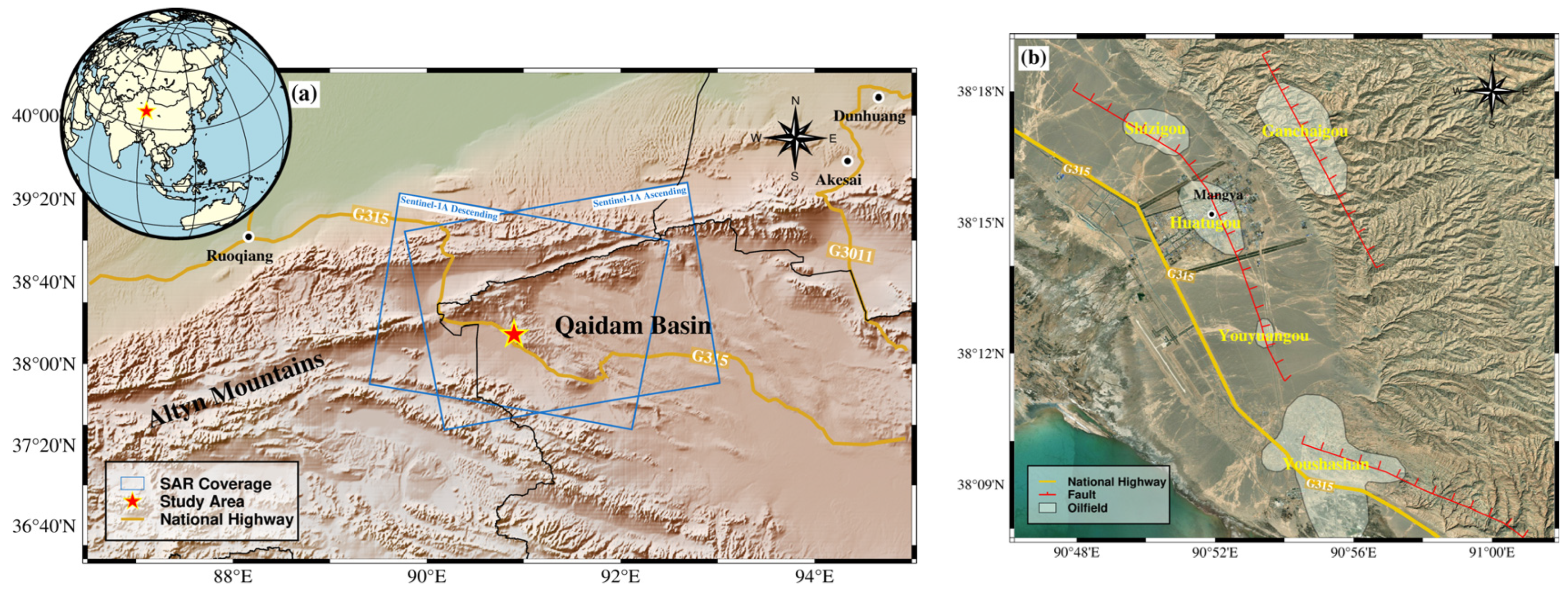
2.1. Background of the Study Area
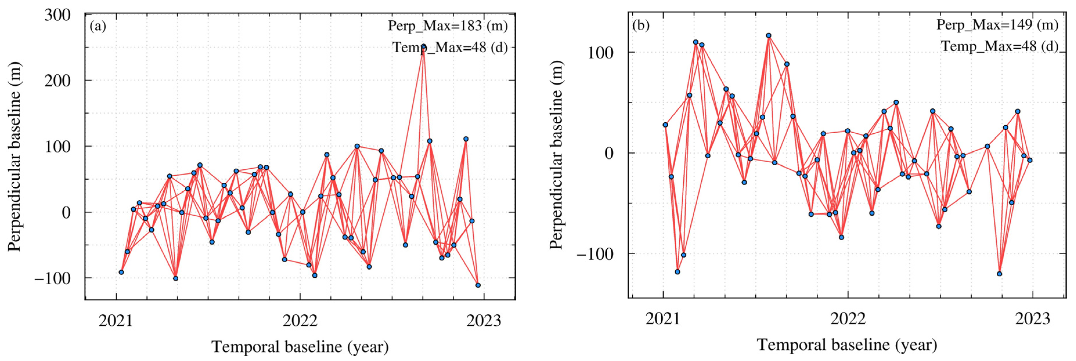
2.2. Data and Processing
3. Methodology
3.1. MSBAS-InSAR Method
3.2. The Source Model and Inversion Method
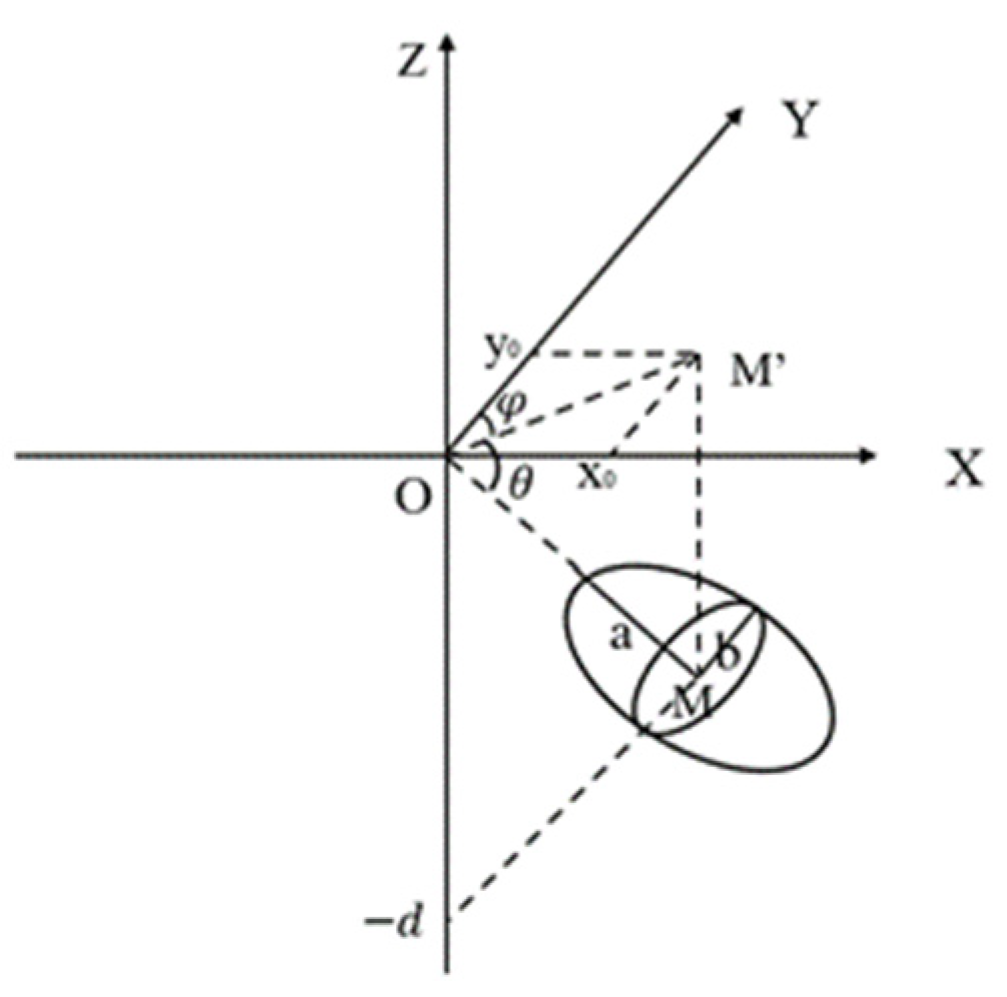
3.2.1. Finite Prolate Spheroidal Model
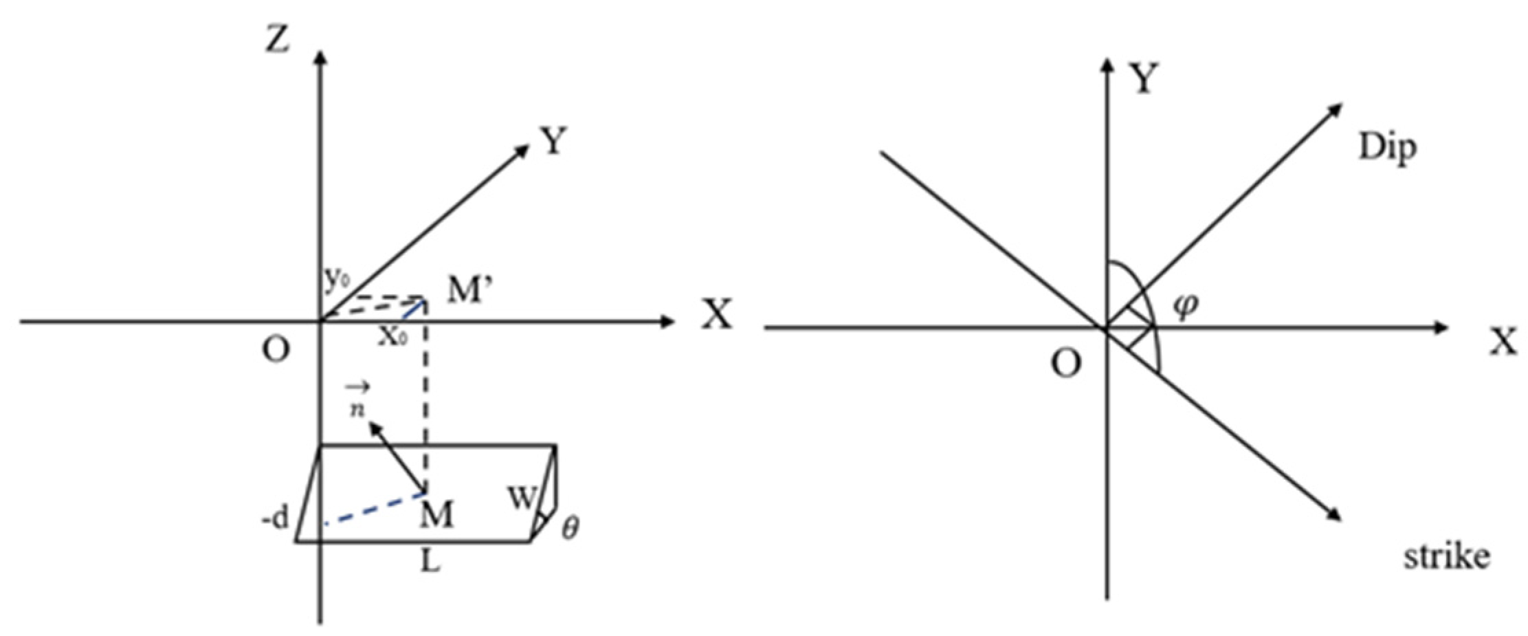
3.2.2. Dipping Dike with Uniform Opening Model
3.2.3. The Nonlinear Bayesian Inversion Method
4. Results
4.1. Two-Dimensional (2D) Deformation Monitoring and Analysis
4.2. Reservoir Modeling
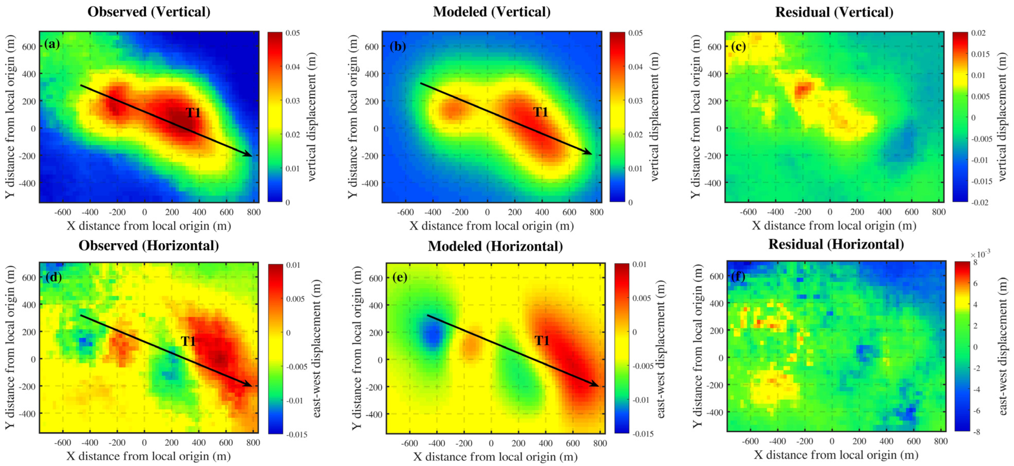
4.2.1. Inversion Result of Area B
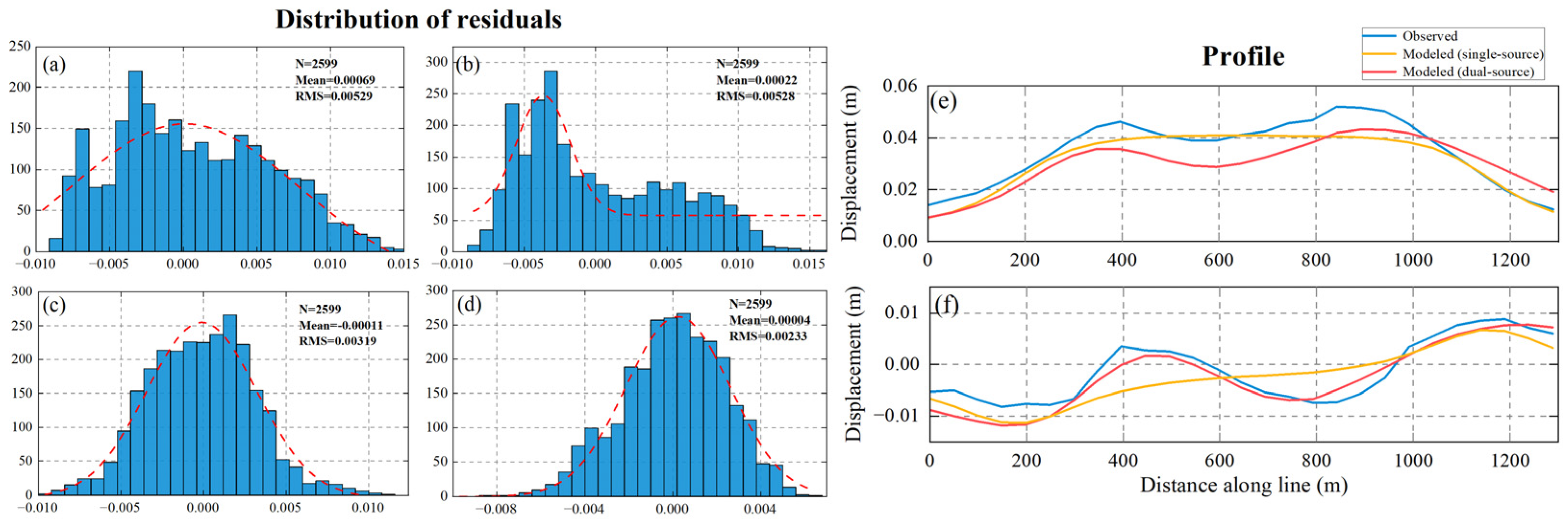
4.2.2. Comparative Analysis of Inversion Results for Area B
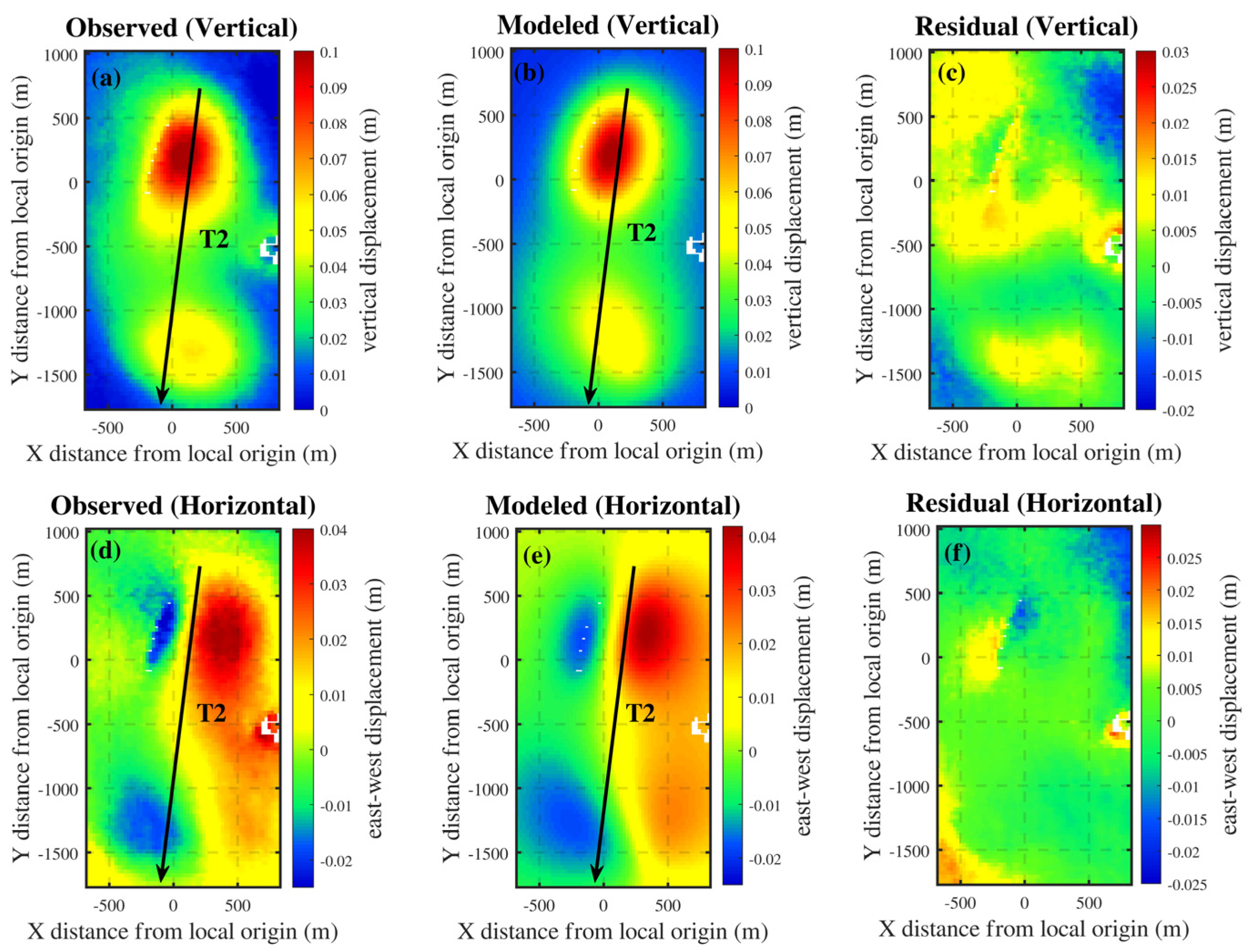
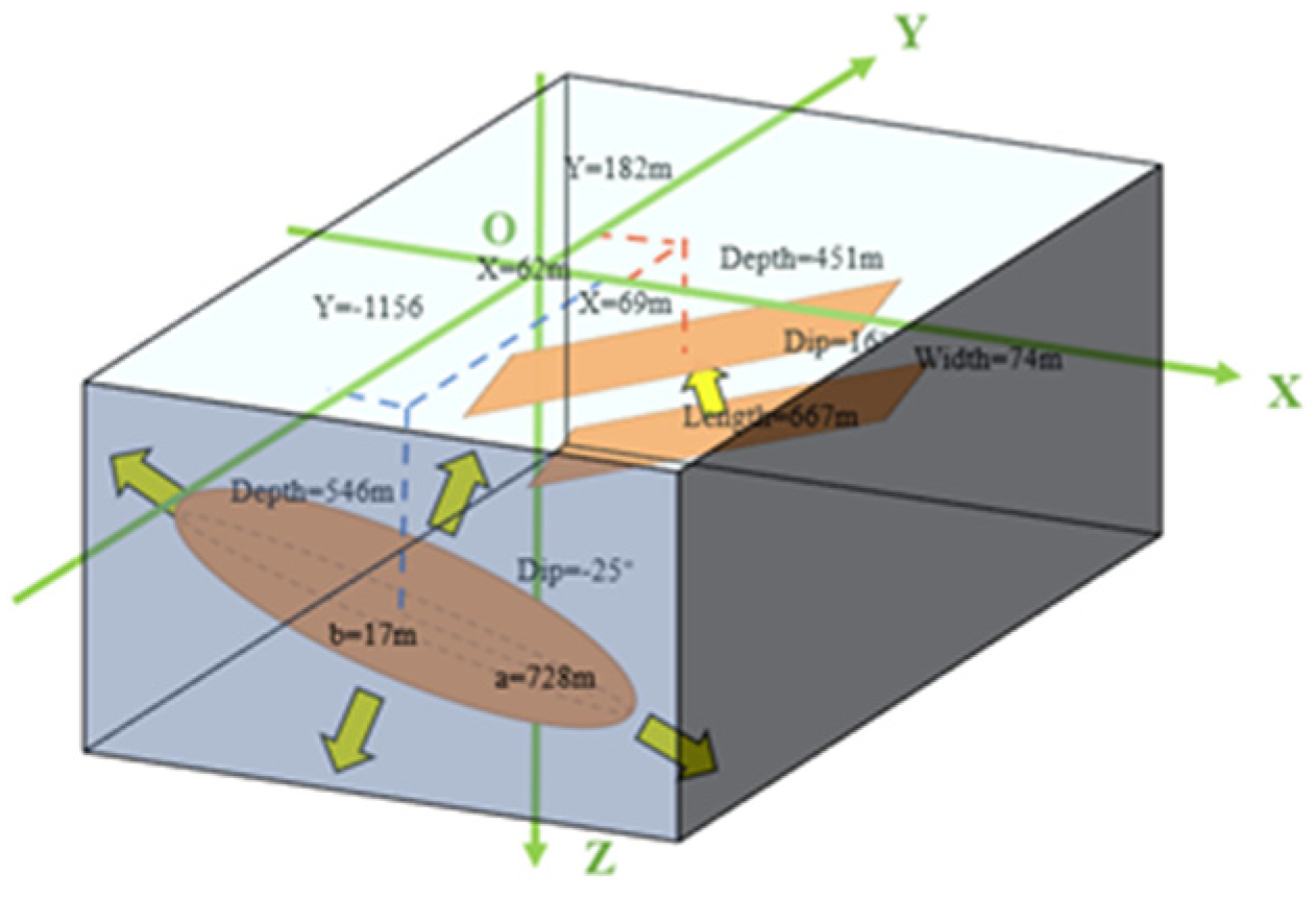
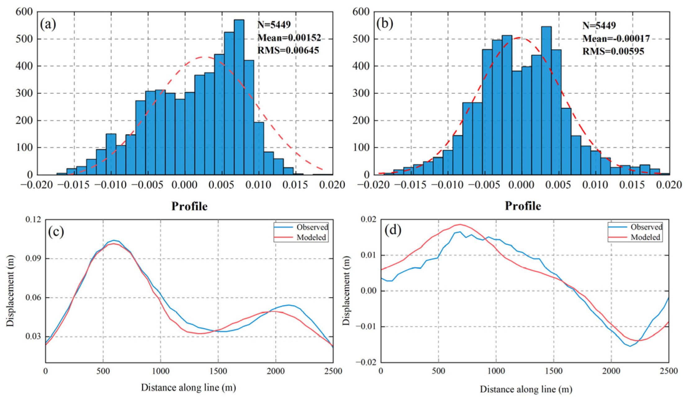
4.2.3. Inversion Results for Area C
5. Discussion
6. Conclusions
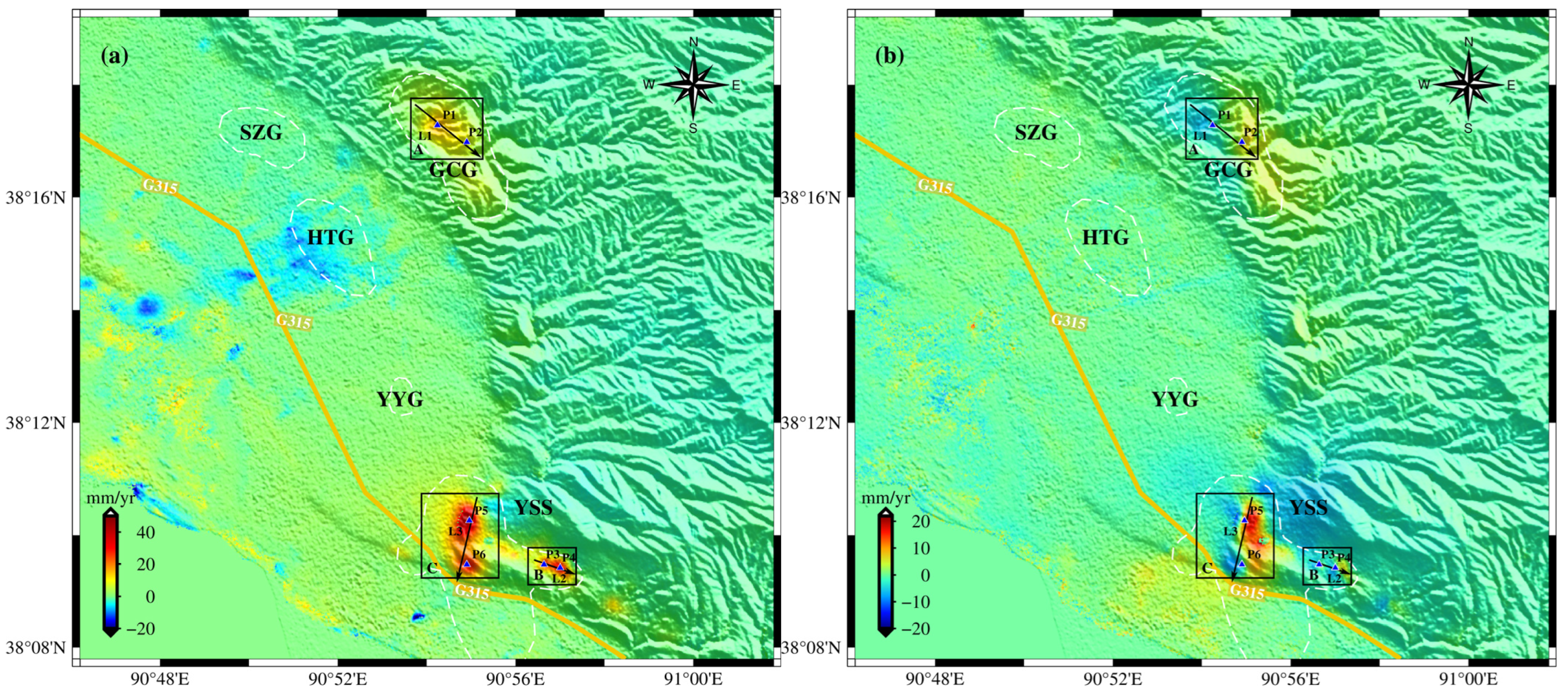
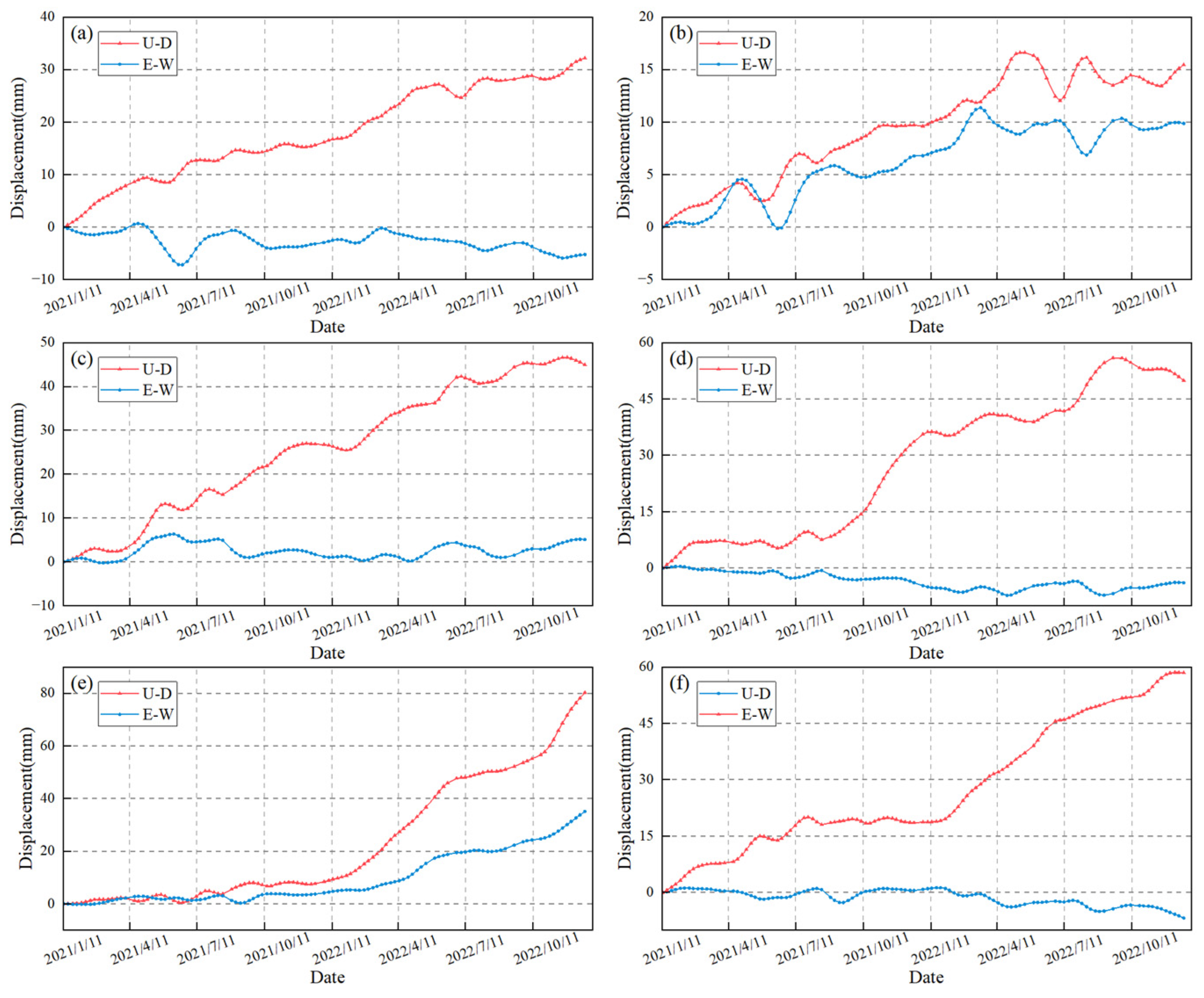
- In the study area, the HTG oilfield exhibited uneven ground subsidence, with a maximum subsidence rate of 12 mm/year. At the same time, the GCG oilfield and YSS oilfield experienced substantial ground uplift, with a maximum rate of 48 mm/year. Along with this uplift process, the east–west deformation rate in this area also reached 16 mm/year. The cause of the ground uplift in the oilfield may be related to increased reservoir pore pressure resulting from water injection. Changes in water injection intensity may lead to changes in deformation rates.
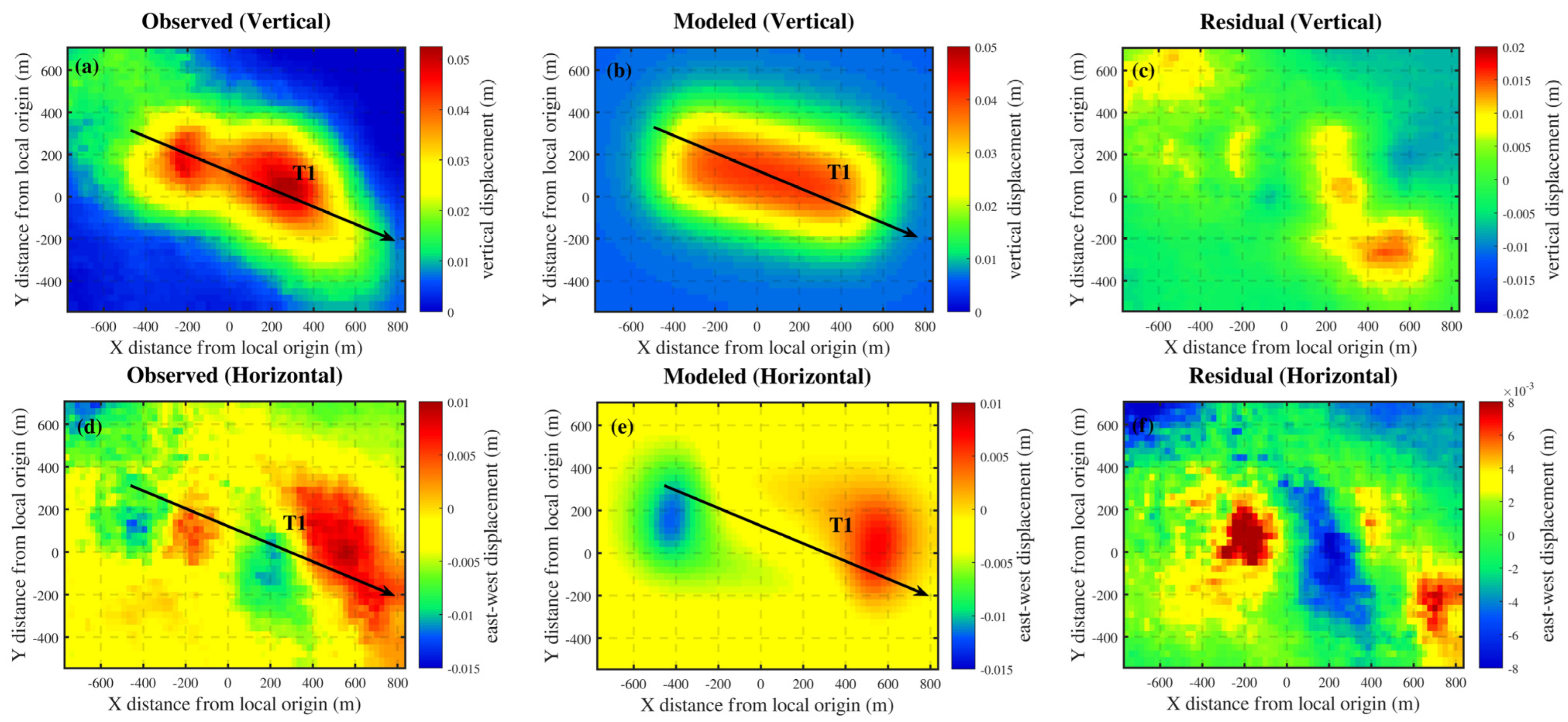
- Combining the analysis of the inversion results, it can be concluded that the introduction of a two-dimensional deformation field helps improve the non-uniqueness of the inversion results, enhance the robustness of the inversion process and, consequently, obtain more reliable oil reservoir parameters. Furthermore, the dual-source model is more suitable for inverting reservoir parameters of complex deformation compared to the single-source model.
Author Contributions
Funding
Data Availability Statement
Acknowledgments
Conflicts of Interest
References
- Pereira, L.B.; Sad, C.M.S.; Castro, E.V.R.; Filgueiras, P.R.; Lacerda, V. Environmental Impacts Related to Drilling Fluid Waste and Treatment Methods: A Critical Review. Fuel 2022, 310, 122301. [Google Scholar] [CrossRef]
- Weijermars, R. Surface Subsidence and Uplift Resulting from Well Interventions Modeled with Coupled Analytical Solutions: Application to Groningen Gas Extraction (Netherlands) and CO2-EOR in the Kelly-Snyder Oil Field (West Texas). Geoenergy Sci. Eng. 2023, 228, 211959. [Google Scholar] [CrossRef]
- Kotsakis, A.; Boukli, A. Transversal Harm, Regulation, and the Tolerance of Oil Disasters. Transnatl. Environ. Law 2023, 12, 71–94. [Google Scholar] [CrossRef]
- Yang, C.; Zhang, D.; Zhao, C.; Han, B.; Sun, R.; Du, J.; Chen, L. Ground Deformation Revealed by Sentinel-1 MSBAS-InSAR Time-Series over Karamay Oilfield, China. Remote Sens. 2019, 11, 2027. [Google Scholar] [CrossRef]
- Ji, L.; Zhang, Y.; Wang, Q.; Xin, Y.; Li, J. Detecting Land Uplift Associated with Enhanced Oil Recovery Using InSAR in the Karamay Oil Field, Xinjiang, China. Int. J. Remote Sens. 2016, 37, 1527–1540. [Google Scholar] [CrossRef]
- Wu, H.; Zhang, Z.; Liu, S.; Wang, Z.; Zhuo, Q.; Lu, X.; Liu, H. Controlling Factors of Hydrocarbon Accumulation and Differential Distribution in the Western Qaidam Basin, Tibet Plateau. Aust. J. Earth Sci. 2022, 69, 591–604. [Google Scholar] [CrossRef]
- Liu, Z.; Zhu, C.; Li, S.; Xue, J.; Gong, Q.; Wang, Y.; Wang, P.; Xia, Z.; Song, G. Geological Features and Exploration Fields of Tight Oil in the Cenozoic of Western Qaidam Basin, NW China. Pet. Explor. Dev. 2017, 44, 217–225. [Google Scholar] [CrossRef]
- Wei, Y. Research on Hydrocarbon Accumulation Regularity of Lithologic Reservoirs in Hongliuquan Area of Qaidam Basin. Ph.D. Thesis, China University of Petroleum (East China), Qingdao, China, 2012. [Google Scholar]
- Wei, X.; Sha, W.; Shen, X.; Si, D.; Zhang, G.; Ren, S.; Yang, M. Petroleum Exploration History and Enlightenment in Qaidam Basin. Xinjiang Pet. Geol. 2021, 42, 302–311. [Google Scholar] [CrossRef]
- Zeng, X.; Li, J.; Tian, J.; Wang, B.; Zhou, F.; Wang, C.; Cui, H.; Haihua, Z. Cenozoic Structural Characteristics and Petroleum Geological Significance of the Qaidam Basin. Energy Explor. Exploit. 2023, 41, 879–899. [Google Scholar] [CrossRef]
- Yi, F.; Yi, H.; Mu, C.; Tang, W.; Li, N.; Chen, Y.; Tian, K.; Shi, Y.; Wu, J.; Xia, G. Organic Geochemical Characteristics and Organic Matter Accumulation of the Eocene Lacustrine Source Rock in the Yingxi Area, Western Qaidam Basin, China. Int. J. Earth Sci. 2023, 112, 1277–1292. [Google Scholar] [CrossRef]
- Wu, P.; Wei, M.; D’Hondt, S. Subsidence in Coastal Cities Throughout the World Observed by InSAR. Geophys. Res. Lett. 2022, 49, e2022GL098477. [Google Scholar] [CrossRef]
- Liao, M.; Zhang, R.; Lv, J.; Yu, B.; Pang, J.; Li, R.; Xiang, W.; Tao, W. Subsidence Monitoring of Fill Area in Yan’an New District Based on Sentinel-1A Time Series Imagery. Remote Sens. 2021, 13, 3044. [Google Scholar] [CrossRef]
- Bao, X.; Zhang, R.; Shama, A.; Li, S.; Xie, L.; Lv, J.; Fu, Y.; Wu, R.; Liu, G. Ground Deformation Pattern Analysis and Evolution Prediction of Shanghai Pudong International Airport Based on PSI Long Time Series Observations. Remote Sens. 2022, 14, 610. [Google Scholar] [CrossRef]
- Cai, J.; Zhang, L.; Dong, J.; Dong, X.; Li, M.; Xu, Q.; Liao, M. Detection and Characterization of Slow-Moving Landslides in the 2017 Jiuzhaigou Earthquake Area by Combining Satellite SAR Observations and Airborne Lidar DSM. Eng. Geol. 2022, 305, 106730. [Google Scholar] [CrossRef]
- Cheaib, A.; Lacroix, P.; Zerathe, S.; Jongmans, D.; Ajorlou, N.; Doin, M.-P.; Hollingsworth, J.; Abdallah, C. Landslides Induced by the 2017 Mw7.3 Sarpol Zahab Earthquake (Iran). Landslides 2022, 19, 603–619. [Google Scholar] [CrossRef]
- Zheng, Z.; Xie, C.; He, Y.; Zhu, M.; Huang, W.; Shao, T. Monitoring Potential Geological Hazards with Different InSAR Algorithms: The Case of Western Sichuan. Remote Sens. 2022, 14, 2049. [Google Scholar] [CrossRef]
- Ferretti, A.; Prati, C.; Rocca, F. Permanent Scatterers in SAR Interferometry. IEEE Trans. Geosci. Remote Sens. 2001, 39, 8–20. [Google Scholar] [CrossRef]
- Berardino, P.; Fornaro, G.; Lanari, R.; Sansosti, E. A New Algorithm for Surface Deformation Monitoring Based on Small Baseline Differential SAR Interferograms. IEEE Trans. Geosci. Remote Sens. 2002, 40, 2375–2383. [Google Scholar] [CrossRef]
- Ferretti, A.; Fumagalli, A.; Novali, F.; Prati, C.; Rocca, F.; Rucci, A. A New Algorithm for Processing Interferometric Data-Stacks: SqueeSAR. IEEE Trans. Geosci. Remote Sens. 2011, 49, 3460–3470. [Google Scholar] [CrossRef]
- Fornaro, G.; Verde, S.; Reale, D.; Pauciullo, A. CAESAR: An Approach Based on Covariance Matrix Decomposition to Improve Multibaseline–Multitemporal Interferometric SAR Processing. IEEE Trans. Geosci. Remote Sens. 2015, 53, 2050–2065. [Google Scholar] [CrossRef]
- Fornaro, G.; Pauciullo, A.; Reale, D.; Verde, S. SAR Coherence Tomography: A New Approach for Coherent Analysis of Urban Areas. In Proceedings of the 2013 IEEE International Geoscience and Remote Sensing Symposium-IGARSS, Melbourne, Australia, 21–26 July 2013; pp. 73–76. [Google Scholar]
- Pierdicca, N.; Maiello, I.; Sansosti, E.; Venuti, G.; Barindelli, S.; Ferretti, R.; Gatti, A.; Manzo, M.; Monti-Guarnieri, A.V.; Murgia, F.; et al. Excess Path Delays From Sentinel Interferometry to Improve Weather Forecasts. IEEE J. Sel. Top. Appl. Earth Obs. Remote Sens. 2020, 13, 3213–3228. [Google Scholar] [CrossRef]
- Wang, T.; Zhang, R.; Zhan, R.; Shama, A.; Liao, M.; Bao, X.; He, L.; Zhan, J. Subsidence Monitoring and Mechanism Analysis of Anju Airport in Suining Based on InSAR and Numerical Simulation. Remote Sens. 2022, 14, 3759. [Google Scholar] [CrossRef]
- Shi, J.; Yang, H.; Peng, J.; Wu, L.; Xu, B.; Liu, Y.; Zhao, B. InSAR Monitoring and Analysis of Ground Deformation Due to Fluid or Gas Injection in Fengcheng Oil Field, Xinjiang, China. J. Indian Soc. Remote Sens. 2019, 47, 455–466. [Google Scholar] [CrossRef]
- Zhang, Y.; Xiang, W.; Liu, G.; Wang, X.; Zhang, R.; Zhang, X.; Tong, J.; Yuan, H.; Zhang, C. Geodetic Imaging of Ground Deformation and Reservoir Parameters at the Yangbajing Geothermal Field, Tibet, China. Geophys. J. Int. 2023, 234, 379–394. [Google Scholar] [CrossRef]
- Chen, Y.; Tong, Y.; Tan, K. Coal Mining Deformation Monitoring Using SBAS-InSAR and Offset Tracking: A Case Study of Yu County, China. IEEE J. Sel. Top. Appl. Earth Obs. Remote Sens. 2020, 13, 6077–6087. [Google Scholar] [CrossRef]
- Sun, H.; Zhang, Q.; Zhao, C.; Yang, C.; Sun, Q.; Chen, W. Monitoring Land Subsidence in the Southern Part of the Lower Liaohe Plain, China with a Multi-Track PS-InSAR Technique. Remote Sens. Environ. 2017, 188, 73–84. [Google Scholar] [CrossRef]
- Juncu, D.; Árnadóttir, T.; Hooper, A.; Gunnarsson, G. Anthropogenic and Natural Ground Deformation in the Hengill Geothermal Area, Iceland. J. Geophys. Res. Solid Earth 2017, 122, 692–709. [Google Scholar] [CrossRef]
- Chen, Y.; Yu, S.; Tao, Q.; Liu, G.; Wang, L.; Wang, F. Accuracy Verification and Correction of D-InSAR and SBAS-InSAR in Monitoring Mining Surface Subsidence. Remote Sens. 2021, 13, 4365. [Google Scholar] [CrossRef]
- Klemm, H.; Quseimi, I.; Novali, F.; Ferretti, A.; Tamburini, A. Monitoring Horizontal and Vertical Surface Deformation over a Hydrocarbon Reservoir by PSInSAR. First Break 2010, 28, 29–37. [Google Scholar] [CrossRef]
- Yang, Q.; Zhao, W.; Dixon, T.H.; Amelung, F.; Han, W.S.; Li, P. InSAR Monitoring of Ground Deformation Due to CO2 Injection at an Enhanced Oil Recovery Site, West Texas. Int. J. Greenh. Gas Control 2015, 41, 20–28. [Google Scholar] [CrossRef]
- Feng, W.; Li, Z.; Hoey, T.; Zhang, Y.; Wang, R.; Samsonov, S.; Li, Y.; Xu, Z. Patterns and Mechanisms of Coseismic and Postseismic Slips of the 2011 M W 7.1 Van (Turkey) Earthquake Revealed by Multi-Platform Synthetic Aperture Radar Interferometry. Tectonophysics 2014, 632, 188–198. [Google Scholar] [CrossRef]
- Wang, Z.; Zhang, R.; Liu, Y. 3D Coseismic Deformation Field and Source Parameters of the 2017 Iran-Iraq Mw7.3 Earthquake Inferred from DInSAR and MAI Measurements. Remote Sens. 2019, 11, 2248. [Google Scholar] [CrossRef]
- Wu, L.; Xiao, A.; Ma, D.; Li, H.; Xu, B.; Shen, Y.; Mao, L. Cenozoic Fault Systems in Southwest Qaidam Basin, Northeastern Tibetan Plateau: Geometry, Temporal Development, and Significance for Hydrocarbon Accumulation. Bulletin 2014, 98, 1213–1234. [Google Scholar] [CrossRef]
- Wegnüller, U.; Werner, C.; Strozzi, T.; Wiesmann, A.; Frey, O.; Santoro, M. Sentinel-1 Support in the GAMMA Software. Procedia Comput. Sci. 2016, 100, 1305–1312. [Google Scholar] [CrossRef]
- Cascini, L.; Fornaro, G.; Peduto, D. Advanced Low- and Full-Resolution DInSAR Map Generation for Slow-Moving Landslide Analysis at Different Scales. Eng. Geol. 2010, 112, 29–42. [Google Scholar] [CrossRef]
- Samsonov, S.; d’Oreye, N.; Smets, B. Ground Deformation Associated with Post-Mining Activity at the French–German Border Revealed by Novel InSAR Time Series Method. Int. J. Appl. Earth Obs. Geoinf. 2013, 23, 142–154. [Google Scholar] [CrossRef]
- Samsonov, S.V.; d’Oreye, N. Multidimensional Small Baseline Subset (MSBAS) for Two-Dimensional Deformation Analysis: Case Study Mexico City. Can. J. Remote Sens. 2017, 43, 318–329. [Google Scholar] [CrossRef]
- Hansen, P.C. The truncatedSVD as a Method for Regularization. BIT 1987, 27, 534–553. [Google Scholar] [CrossRef]
- Matsu’Ura, M. Inversion of Geodetic Data. I. Mathematical Formulation. J. Phys. Earth 1977, 25, 69–90. [Google Scholar] [CrossRef]
- Yang, X.-M.; Davis, P.M.; Dieterich, J.H. Deformation from Inflation of a Dipping Finite Prolate Spheroid in an Elastic Half-Space as a Model for Volcanic Stressing. J. Geophys. Res. 1988, 93, 4249–4257. [Google Scholar] [CrossRef]
- Okada, Y. Surface Deformation Due to Shear and Tensile Faults in a Half-Space. Bull. Seismol. Soc. Am. 1985, 75, 1135–1154. [Google Scholar] [CrossRef]
- Okada, Y. Internal Deformation Due to Shear and Tensile Faults in a Half-Space. Bull. Seismol. Soc. Am. 1992, 82, 1018–1040. [Google Scholar] [CrossRef]
- Du, Z. Theory and Application of Geodesy Inversion Based on Mechanical Models. Acta Geod. Cartogr. Sin. 2002, 31, 94. [Google Scholar] [CrossRef]
- Bagnardi, M.; Hooper, A. Inversion of Surface Deformation Data for Rapid Estimates of Source Parameters and Uncertainties: A Bayesian Approach. Geochem. Geophys. Geosystems 2018, 19, 2194–2211. [Google Scholar] [CrossRef]
- Hastings, W.K. Monte Carlo Sampling Methods Using Markov Chains and Their Applications. Biometrika 1970, 57, 97–109. [Google Scholar] [CrossRef]
- Mosegaard, K.; Tarantola, A. Monte Carlo Sampling of Solutions to Inverse Problems. J. Geophys. Res. 1995, 100, 12431–12447. [Google Scholar] [CrossRef]
- Mogi, K. Relations between the Eruptions of Various Volcanoes and the Deformations of the Ground Surfaces around Them. Bull. Earthq. Res. Inst. 1958, 36, 99–134. [Google Scholar]


| Sensor | Wavelength | Azimuth/Range Pixel Spacing | Orbit Direction | Path | Temporal Coverage |
|---|---|---|---|---|---|
| Sentinel-1A | 5.6 cm | 13.99 m/2.33 m | Ascending | 143 | 11 January 2021–20 December 2022 |
| Descending | 48 | 5 January 2021–26 December 2022 |
| Source | Source Parameter | Optimal Value | Confidence Interval (2.5%) | Confidence Interval (97.5%) |
|---|---|---|---|---|
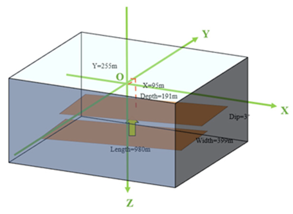
| Rectangular dislocation surface | Length (m) | 980.668 | 956.542 | 1016.85 |
| Width (m) | 399.642 | 372.435 | 433.755 | |
| X | 95.1182 | 78.7143 | 117.508 | |
| Y | 255.5 | 232.037 | 279.799 | |
| Depth (m) | 191.863 | 171.431 | 227.192 | |
| Strike (°) | −77.5828 | −79.791 | −74.8579 | |
| Dip (°) | 3.20863 | −0.540244 | −8.16204 | |
| Opening | 0.04148 | 0.03741 | 0.04697 |
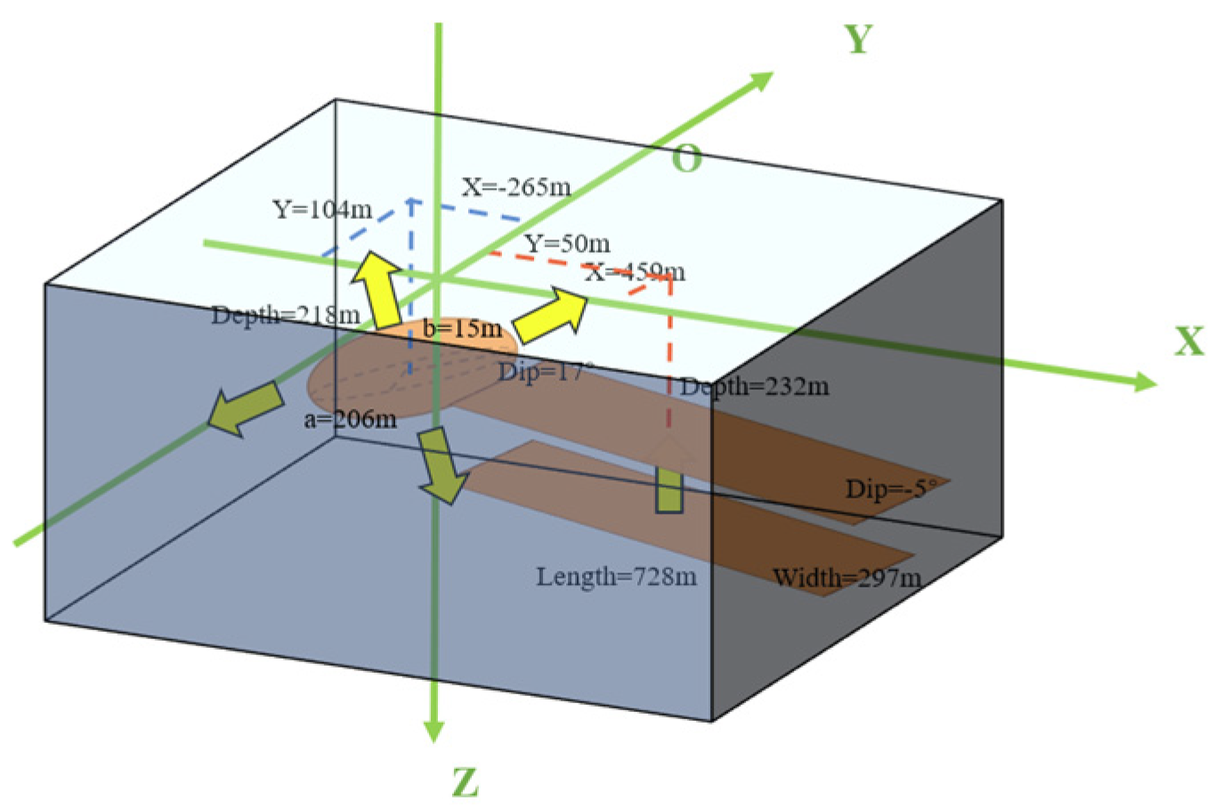
| Source | Source Parameter | Optimal Value | Confidence Interval (2.5%) | Confidence Interval (97.5%) |
|---|---|---|---|---|
| Dipping ellipsoid | X | −265.211 | −288.02 | −246.469 |
| Y | 104.859 | 87.0402 | 126.723 | |
| Depth (m) | 218.904 | 194.592 | 246.927 | |
| Major semi-axis (m) | 206.595 | 168.143 | 252.8 | |
| Minor semi-axis (m) | 15.0091 | 6.77208 | 55.16096 | |
| Strike (°) | 65.0119 | 46.6214 | 75.1686 | |
| Dip (°) | 17.5249 | 10.5561 | 27.3211 | |
| DP/mu | 0.03467 | 0.00378 | 0.09103 | |
| Rectangular dislocation surface | Length (m) | 728.471 | 637.649 | 777.356 |
| Width (m) | 297.448 | 204.269 | 333.208 | |
| X | 459.077 | 413.4 | 476.708 | |
| Y | 50.9312 | 17.552 | 80.1817 | |
| Depth (m) | 232.529 | 211.876 | 286.603 | |
| Strike (°) | −39.4342 | −43.6891 | −34.872 | |
| Dip (°) | −5.77362 | −11.5944 | −0.41442 | |
| Opening (m) | 0.06292 | 0.05257 | 0.09577 |
| Source | Source Parameter | Optimal Value | Confidence Interval (2.5%) | Confidence Interval (97.5%) |
|---|---|---|---|---|
| Rectangular dislocation surface | Length (m) | 667.166 | 39.456 | 703.224 |
| Width (m) | 74.3788 | 35.9698 | 87.6175 | |
| X | 69.8736 | 44.1824 | 84.5374 | |
| Y | 182.243 | 170.078 | 194.093 | |
| Depth (m) | 451.511 | 441.582 | 468.684 | |
| Strike (°) | 15.2082 | 13.0072 | 17.5933 | |
| Dip (°) | 16.0407 | 11.3015 | 19.5505 | |
| Opening (m) | 1.15447 | 1.01517 | 2.39906 | |
| Dipping ellipsoid | X | 61.8081 | 35.3234 | 151.877 |
| Y | −1156.77 | −1341.57 | −1113.89 | |
| Depth (m) | 546.16 | 492.207 | 598.769 | |
| Major semi-axis (m) | 728.4 | 334.435 | 792.369 | |
| Minor semi-axis (m) | 17.2557 | 3.82994 | 55.9840 | |
| Strike (°) | 151.538 | 82.9156 | 158.568 | |
| Dip (°) | −25.2426 | −29.3177 | −9.12962 | |
| DP/mu | 0.07786 | 0.01098 | 0.358436 |
Disclaimer/Publisher’s Note: The statements, opinions and data contained in all publications are solely those of the individual author(s) and contributor(s) and not of MDPI and/or the editor(s). MDPI and/or the editor(s) disclaim responsibility for any injury to people or property resulting from any ideas, methods, instructions or products referred to in the content. |
© 2023 by the authors. Licensee MDPI, Basel, Switzerland. This article is an open access article distributed under the terms and conditions of the Creative Commons Attribution (CC BY) license (https://creativecommons.org/licenses/by/4.0/).
Share and Cite
Liu, A.; Zhang, R.; Yang, Y.; Wang, T.; Wang, T.; Shama, A.; Zhan, R.; Bao, X. Oilfield Reservoir Parameter Inversion Based on 2D Ground Deformation Measurements Acquired by a Time-Series MSBAS-InSAR Method. Remote Sens. 2024, 16, 154. https://doi.org/10.3390/rs16010154
Liu A, Zhang R, Yang Y, Wang T, Wang T, Shama A, Zhan R, Bao X. Oilfield Reservoir Parameter Inversion Based on 2D Ground Deformation Measurements Acquired by a Time-Series MSBAS-InSAR Method. Remote Sensing. 2024; 16(1):154. https://doi.org/10.3390/rs16010154
Chicago/Turabian StyleLiu, Anmengyun, Rui Zhang, Yunjie Yang, Tianyu Wang, Ting Wang, Age Shama, Runqing Zhan, and Xin Bao. 2024. "Oilfield Reservoir Parameter Inversion Based on 2D Ground Deformation Measurements Acquired by a Time-Series MSBAS-InSAR Method" Remote Sensing 16, no. 1: 154. https://doi.org/10.3390/rs16010154
APA StyleLiu, A., Zhang, R., Yang, Y., Wang, T., Wang, T., Shama, A., Zhan, R., & Bao, X. (2024). Oilfield Reservoir Parameter Inversion Based on 2D Ground Deformation Measurements Acquired by a Time-Series MSBAS-InSAR Method. Remote Sensing, 16(1), 154. https://doi.org/10.3390/rs16010154