A General Deep Learning Point–Surface Fusion Framework for RGB Image Super-Resolution

Abstract

Hyperspectral images are usually acquired in a scanning-based way, which can cause inconvenience in some situations. In these cases, RGB image spectral super-resolution technology emerges as an alternative. However, current mainstream spectral super-resolution methods aim to generate continuous spectral information at a very narrow range, limited to the visible light range. Some researchers introduce hyperspectral images as auxiliary data. But it is usually required that the auxiliary hyperspectral images have the same spatial range as RGB images. To address this issue, a general point–surface data fusion method is designed to achieve the RGB image spectral super-resolution goal in this paper, named GRSS-Net. The proposed method utilizes hyperspectral point data as auxiliary data to provide spectral reference information. Thus, the spectral super-resolution can extend the spectral reconstruction range according to spectral data. The proposed method utilizes compressed sensing theory as a fundamental physical mechanism and then unfolds the traditional hyperspectral image reconstruction optimization problem into a deep network. Finally, a high-spatial-resolution hyperspectral image can be obtained. Thus, the proposed method combines the non-linear feature extraction ability of deep learning and the interpretability of traditional physical models simultaneously. A series of experiments demonstrates that the proposed method can effectively reconstruct spectral information in RGB images. Meanwhile, the proposed method provides a framework of spectral super-resolution for different applications.

1. Introduction

Hyperspectral images carry abundant spectral information. The spectral information contains reflection features, which can uncover the composition of different ground objects [1,2,3]. Benefiting from such recognition ability, hyperspectral images can promote the accuracy of many applications, such as large-area ground object classification [4], anomaly target detection [5], etc.

Hyperspectral images can be acquired by pushbroom or sweeping spectrometers. However, the scanning-based hyperspectral image collection pattern is not very friendly to some objects that are difficult to scan, for example, enormous, tiny, or irregular objects. Snapshot hyperspectral imaging can solve this issue to some extent [6]. But this technology is still developing and has not been widely promoted yet. In addition, the platforms equipped with hyperspectral sensors are usually bulky. This limits the flexibility of obtaining hyperspectral images. In contrast, RGB image acquisition is more flexible. Thanks to the rapid development of computer image processing technology, spectral super-resolution using RGB images to generate high-spatial-resolution hyperspectral (HRHS) images can already be achieved [7,8,9,10]. However, this is a severely ill-posed problem and it cannot be solved by commonly used probability statistics methods [11]. From the perspective of employed methods, current spectral super-resolution approaches can be divided into two categories [12,13]: (1) Methods based on compressive imaging or sparse reconstruction [14,15]. These kinds of methods use the property of image compressibility. Some typical algorithms, such as that of Arad et al. [9], construct a spectral recovery method using a sparse coding method, which collects plenty of hyperspectral images as prior knowledge; (2) Methods based on deep learning [16,17]. These algorithms use deep learning technology to achieve effective mapping from low-dimensional RGB image space to high-dimensional hyperspectral image space. A typical algorithm, such as that of Zhu et al. [18], uses deep learning-based architecture to improve an interpretable network, named AGD-Net. This network performs spatial and spectral feature extraction based on the low-rank prior of hyperspectral images and then uses a network combining amended gradient descent and deep learning architecture to achieve spectral reconstruction. According to whether they use hyperspectral images as prior knowledge, spectral super-resolution methods can be classified into two types [19,20]: (1) Methods that only utilize RGB images. These methods utilize some mapping methods, such as multiple linear regression or deep learning, to obtain the specific mapping relationship between RGB images and hyperspectral images from training datasets. Then, the trained model can be used to map pure RGB images to HRHS images; (2) Methods that utilize hyperspectral images as prior knowledge. The main idea of this type of method is to extract high-resolution spatial and spectral information from RGB images and hyperspectral images, respectively, and then fuse them to generate HRHS images [21,22]. There have been many related studies on these methods, such as Hang et al. [23], who designed the PriNET+ network to obtain HRHS images according to the intrinsic properties of hyperspectral images. However, spectral super-resolution methods using only RGB images focus on the visible spectral range, because the spectral range of RGB images is very limited, only containing the visible range. Some researchers introduce hyperspectral images to assist in extending the reconstructed spectral range, that is, the methods utilizing hyperspectral images as prior knowledge. For example, Li et al. [24] developed a BUSIFusion network, which uses an unrolling network and coordinate encoding to achieve RGB and hyperspectral image fusion and obtain HRHS images. Gao et al. [25] proposed a spectral super-resolution algorithm, named J-SLoL, which uses small-area hyperspectral images and large-area multispectral images to obtain large-area HRHS images based on sparse and low-rank learning. Although massive spectral super-resolution methods have been developed, there still exist some technique challenges: (1) The reconstructed spectral range of methods that only require RGB images is limited; (2) The assisted hyperspectral image usually requires an overlapped or partially overlapped spatial range with an RGB image; (3) The pure deep learning-based method has massive training parameters and a high computational cost. In addition, the physical meaning of deep learning-based methods is undisclosed.

On the basis of the above-mentioned shortcomings of current spectral super-resolution method development, replacing the auxiliary hyperspectral images with hyperspectral point data would be more convenient. Thus, the spectral super-resolution problem can be converted into how to inject hyperspectral information into RGB images. Pure deep learning-based methods make it difficult to accomplish the mapping between point data and image data, as their spatial and spectral dimensions are not equal. Traditional methods, such as sparse coding, can only complete linear mapping. Therefore, a general interpretable point–surface fusion deep network architecture for RGB image spectral super-resolution is proposed in this paper, named GRSS-Net. The GRSS-Net uses hyperspectral point data as auxiliary data. In the proposed method, RGB images and some spectral data of ground objects in a targeted scene are needed. RGB images provide detailed spatial information and spectral data provide abundant spectral information. Then, basic compressed sensing theory is used to describe the entire spectral reconstruction process and to construct the optimization problem. Subsequently, the optimization method is used and the entire solution process is designed as a network.

In conclusion, the main contributions of the proposed method compared with traditional spectral super-resolution methods can be summarized as follows:

(1)

The proposed method has both the non-linear feature extraction ability of deep learning and the interpretability and clarity of the physical model;

(2)

With the help of spectral data, the proposed method can save time and effort in obtaining HRHS images that are not limited to the visible light range;

(3)

Compared with pure deep learning-based methods, GRSS-Net requires fewer training parameters and does not need image registration;

(4)

More importantly, the proposed method provides a point–surface fusion framework, which can solve the problem of difficulty in obtaining hyperspectral images effectively.

The remaining content of this paper is arranged as follows. Section 2 lists some background research work related to this paper and the fundamental principle of the proposed method. Next, Section 3 displays validation experiments and results, followed by Section 4, which provides a discussion to further verify the adaptability of the proposed method. Finally, the conclusion of the entire paper is given in Section 5.

2. Methodology

2.1. Related Work

This subsection introduces some background knowledge related to the proposed method, including the underlying physical model of the proposed algorithm, which is the compressed sensing and optimization method used in this paper.

2.1.1. Compressed Sensing

The gist of compressed sensing theory is that if the signal is sparse, it can be reconstructed and restored from very few samples. In other words, the original signal can be compressed. The mathematical expression is organized as follows:

$$\mathit{Y}=\phi \mathit{S},$$

(1)

where Y is observed data, which is resampled data; $\phi$ represents the observation matrix, which is used to implement sampling regulation; S is the original data before sampling.

Assuming that the original signal is not sparse, that is, there is not a significant proportion of zero value in the original signal, some sparse decomposition must be implemented before carrying out compressing [26]. The sparse decomposition process can be formulated as follows:

$$\mathit{Y}=\phi Ds,$$

(2)

where matrix D represents the sparse basis vectors used to complete sparse transformation; s is the sparse transformation/sparse coding matrix, through which the original signal S can be converted into a sparse signal.

For Equation (2), there is a vital prerequisite, which is that the observation matrix $\phi$ and the basis vector matrix D must be unrelated [27].

Through Equation (2), the original signal S can be converted to sparse form. Meanwhile, the main valid information of S can be stored in matrices $\phi$, D, and s.

The compressed signal occupies less memory, making it more convenient for transmission and calculation, especially for batch data. When the original signal is needed, some signal recovery method can be used to reconstruct the original signal. The signal reconstruction-solving process can be abstracted as an optimization problem as follows:

$$s=arg \min \Vert \phi Ds-\mathit{Y}{\Vert }^2+\lambda \Vert s{\Vert }_1,$$

(3)

where $\lambda$ is the coefficient of constraint.

The optimization algorithms used in signal reconstruction can be summarized into the following three categories: (1) Greedy algorithms, such as orthogonal matching pursuit (OMP); (2) Iterative threshold algorithms, for example, iterative shrinkage threshold algorithm (ISTA); (3) A combination of algorithms.

2.1.2. Gradient Descent

Gradient descent is a search-based optimization algorithm, which can be used to solve least-squares problems without constraints. When searching for the minimum value of an object function, the gradient descent method can be used to iteratively solve it step by step [28]. Finally, the minimum object function and the optimal model parameter value can be obtained.

The detailed calculation can be formulated as follows:

$$x_{k+1}=x_k-2t\nabla f\left(x_k\right),$$

(4)

$$\nabla f\left(x_k\right)=\frac{\partial f\left(x_k\right)}{\partial x_k},$$

(5)

where x is the variable required to find the optimal solution; t is the appropriate step size.

2.1.3. Iterative Soft-Threshold Shrinkage

Iterative soft-threshold shrinkage is developed on the basis of the gradient descent algorithm, and it can further solve a least-squares problem with an L₁ constraint. Compared with algorithms such as OMP, ISTA has the advantages of simplicity and comprehensibility [29]. Thus, the ISTA algorithm is chosen as the optimization method in this paper. The ISTA is designed to optimize the following problem:

$$x=arg \min \Vert \mathit{A}x-b{\Vert }^2+\lambda \Vert x{\Vert }_1,$$

(6)

where A and b are both known quantities.

For Equation (6), utilizing ISTA to find the optimization solution, the solving formulas can be written as follows:

$$x_{k+1}=pro{x}_{\lambda t}\left(x_k-2t\nabla f\left(x_k\right)\right),$$

(7)

$$pro{x}_{\lambda t}\left(x_k\right)=\left(\left|\left.x_k\right|\right.-\lambda t\right)+\mathrm{sgn}\left(x_k\right),$$

(8)

here, $\nabla f\left(x_k\right)=A^T(A{x}_k-b)$; the $prox(·)$ represents the shrinkage operation; $\mathrm{s}\mathrm{g}\mathrm{n}(·)$ denotes the sign function, which determines whether a variable is positive or negative.

2.2. Observation Model

It is widely recognized that hyperspectral images have low-rank and sparse properties. From the perspective of compressed sensing, hyperspectral images can be compressed. Firstly, the original hyperspectral image can be decomposed into a sparse basis vector matrix and a sparse coding matrix. Then, an observation matrix is used to complete compression. For hyperspectral images, there exist two types of observation matrix: one considers the spatial dimension, and the other is processed from the spectral dimension. Adopting an observation matrix considering the spatial dimension means compressing the original image from the spatial dimension. As a result, a low-spatial-resolution hyperspectral image is generated. Conversely, by compressing the original image from the spectral dimension, an RGB image or a multispectral image is generated. Thus, the observation model of HRHS images ${\mathit{X}}_{HRHS}$ and RGB images ${\mathit{X}}_{RGB}$ can be expressed as follows:

$${\mathit{X}}_{HRHS}=D_{HRHS}\times s_{HRHS},$$

(9)

$${\mathit{X}}_{RGB}={\phi }_{RGB}\times D_{HRHS}\times s_{HRHS},$$

(10)

where ${\phi }_{RGB}$ is the observation matrix from the spectral dimension, whose function is similar to the spectral response function; $D_{HRHS}$ is the spectral basis vector matrix; $s_{HRHS}$ denotes the corresponding sparse coding matrix of $D_{HRHS}$.

The part ${\phi }_{RGB}\times D_{HRHS}$ in Equation (10) can be seen as the three-dimensional mapping of $D_{HRHS}$, which is the three-dimensional basis vector matrix of RGB $D_{RGB}$, thus an RGB image can be re-written as:

$${\mathit{X}}_{RGB}=D_{RGB}\times s_{HRHS}.$$

(11)

The above-mentioned observation model is depicted in Figure 1. It is worth mentioning that spectral data can be seen as the basis vector matrix of an HRHS image. To ensure that the most useful information is retained, the spectral basis vector matrix should contain the spectra of every vital object in the targeted scene as much as possible.

In the final observation model Equation (11), there only exists one unknown variable, which is $s_{HRHS}$. Consequently, the point–surface fusion method-guided RGB spectral super-resolution problem can be converted to searching for the optimized solution of $s_{HRHS}$.

2.3. Fundamental Formula Derivation of GRSS-Net

Based on the observation model proposed in Section 2.2, the object function of matrix $s_{HRHS}$ optimization can be described as follows:

$$s_{HRHS}=arg \min \Vert D_{RGB}\times s_{HRHS}-{\mathit{X}}_{RGB}{\Vert }_F^2+\lambda \Vert s_{HRHS}{\Vert }_1.$$

(12)

In this paper, ISTA is chosen to find the optimal solution of Equation (12). Therefore, the solution can be computed by the following equations:

$$r_k=s_{HRHS}^k-2t{D}_{RGB}^T\left(D_{RGB}{s}_{HRHS}^k-{\mathit{X}}_{RGB}\right),$$

(13)

$$s_{HRHS}^{k+1}=pro{x}_{\lambda t}\left(r_k\right),$$

(14)

$$pro{x}_{\lambda t}\left(r_k\right)=\left(\left|r_k\right|-\lambda t\right)+\mathrm{sgn}\left(r_k\right).$$

(15)

On the basis of the above-mentioned solution procedure, a network architecture is unfolded and designed. The flowchart of the proposed network is described in Figure 2.

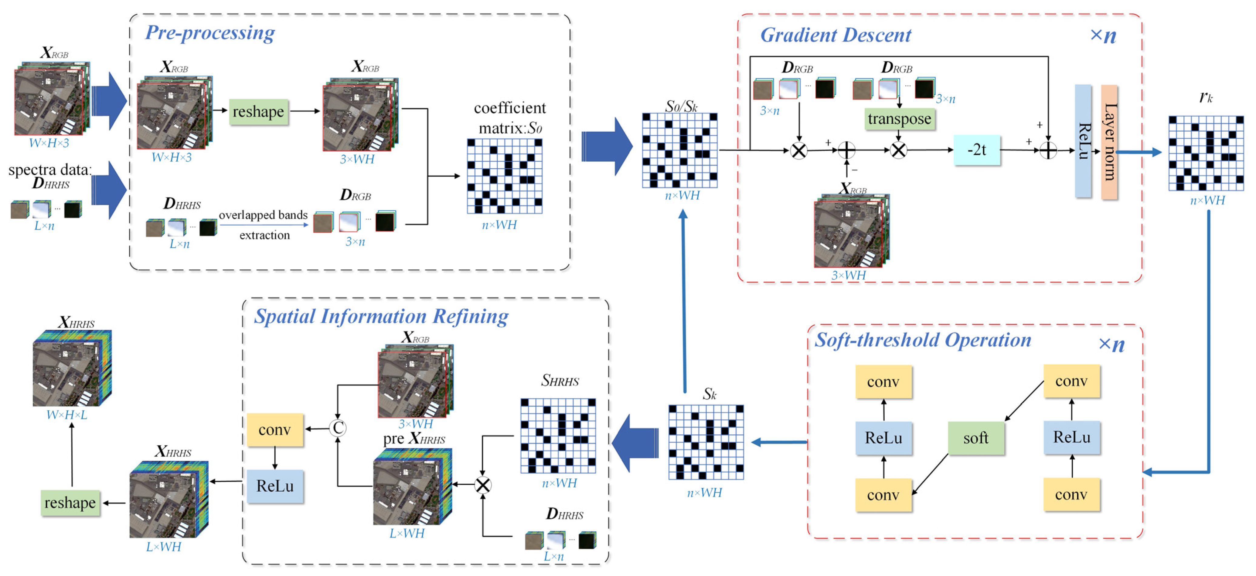
2.4. Architecture of GRSS-Net

The most difficult matter in point–surface fusion is how to effectively inject spectral information into RGB images while maintaining the fidelity of spatial information. In the following content, the solution to this issue will be introduced in detail.

As depicted in Figure 2, the proposed network consists of four main parts: (1) pre-processing; (2) gradient descent calculation; (3) soft-threshold operation; and (4) spatial information refining. In the following content, the detailed implementation process of each module will be introduced.

It should be noted in advance that the iterative optimization process of $s_{HRHS}$ mainly corresponds to the gradient descent calculation and soft-threshold operation modules in GRSS-Net. The gradient descent module is unfolded through Equation (13). Correspondingly, the soft-threshold operation module is unfolded through Equations (13)–(15).

The pre-processing module is designed to initialize $s_{HRHS}$ and $D_{RGB}$. The output of this module is $s_0$, which is the initial value of $s_{HRHS}$, and it is also the input variable of the gradient descent module. Through the gradient descent calculation and soft-threshold operation modules, the optimal solution of $s_{HRHS}$ is obtained. The spatial information-refining module is designed to further organize spatial information. The detailed input and output summary of each module is organized in

Table 1. The input and output of each module.

	Input	Output
pre-processing	${\mathit{X}}_{RGB}$, $D_{HRHS}$	$s_0$, $D_{RGB}$
gradient descent calculation	${\mathit{X}}_{RGB}$, $D_{RGB}$, $s_0/s_k$	$r_k$
soft-threshold operation	$r_k$	$r_k$
spatial information refining	${\mathit{X}}_{RGB}$, $D_{HRHS}$, $s_{HRHS}$	${\mathit{X}}_{HRHS}$

.

In the following sub-subsections, the four modules in GRSS-Net will be presented in detail.

2.4.1. Pre-Processing

In the pre-processing part, all variables are assigned initial values, including the basis vector matrix of RGB images $D_{RGB}$ and the sparse coding matrix $s_0$. To establish the connection between spectral data and RGB images, the basis vector matrix of RGB images can be acquired by extracting three overlapped bands from prior spectral data whose center wavelengths are located on red, green, and blue, respectively. After determining the basis vector matrix $D_{RGB}$, the coefficient matrix to be optimized can be initialized by the least-squares method. The specific formula is as follows:

$$s_0={\left({D_{RGB}}^T{D}_{RGB}\right)}^{-1}{D_{RGB}}^T{\mathit{X}}_{RGB},$$

(16)

where $s_0$ represents the initialized coefficient matrix.

2.4.2. Gradient Descent Calculation

The gradient descent module carries out the gradient calculation operation. In this module, some activation and layer norm layers are used to increase non-linear mapping during calculation.

The output of the pre-processing module is utilized as the input of this module to participate in the calculation. The entire gradient descent calculation follows Equation (13). The parameter involved in this module, step size t, is set as a trainable parameter. In this way, the steps to find the optimal value of parameter t can be omitted. The formula of this module can be depicted as follows:

$$r_k=Norm\left(\mathrm{Re}Lu\left(s_{k-1}-2t\nabla f\left(s_{k-1}\right)\right)\right),$$

(17)

where $\nabla f\left(s_{k-1}\right)=D_{RGB}^T(D_{RGB}{s}_{k-1}-{\mathit{X}}_{RGB})$; $Norm(·)$ and $ReLu(·)$ denote the layer normalization function and the $ReLu$ activation function, respectively.

The added $ReLu$ function can increase non-linearity in the calculation process. The layer normalization function implements a normalization operation. The purpose of normalization is to ensure the coefficient of basis vectors, which are used in reconstructing each pixel, sum-to-one.

2.4.3. Soft-Threshold Operation

The reference [30] has proven that an appropriate convolution combination calculation can enhance the calculation effect of the soft-threshold operation. Thus, the soft-threshold calculation is designed as follows:

$$s_k={\tilde{\mathcal{F}}}_k\left(soft\left({\mathcal{F}}_k\left(r_k\right)\right)\right),$$

(18)

where $r_k$ is the output of the gradient descent calculation module; ${\mathcal{F}}_k=conv(ReLu(conv(·)))$; $\widetilde{{\mathcal{F}}_k}=conv(ReLu(conv(·)))$, $conv(·)$ represents the convolution calculation operation.

The coefficient matrix solution and preliminary HRHS image reconstruction process can be regarded as spectral information injection. The spectral data contain spectral information and the coefficient matrix is responsible for determining the position of spectral information. Through the first three modules, the preliminary HRHS image can be obtained. Next, a spatial information injection module is designed for spatial texture refining.

2.4.4. Spatial Information Refining

Through the above operations, the optimal solution of the coefficient matrix is obtained. Then, by replacing the RGB basis vector matrix with a hyperspectral basis vector matrix in Equation (11), the preliminary HRHS image can be reconstructed:

$${\mathit{X}}_{preHRHS}=D_{HRHS}\times s_{HRHS}.$$

(19)

The RGB image contains abundant and detailed spatial information, which can assist in improving spatial texture information further. Therefore, the spatial information-refining module is designed for refining spatial information in preliminary HRHS images. Firstly, the RGB image and preliminary HRHS image are concatenated by replacing three overlapped bands in the preliminary HRHS image using the RGB image. Then, the convolution operation is utilized to capture and reconstruct spatial features. The above-mentioned calculation process can be formulated as

$${\tilde{\mathit{X}}}_{\mathrm{HRHS}}=concat\left({\mathit{X}}_{RGB}, {\mathit{X}}_{preHRHS}\right),$$

(20)

$${\tilde{\mathit{X}}}_{\mathrm{HRHS}}=conv\left(\mathrm{Re}Lu\left({\tilde{\mathit{X}}}_{\mathrm{HRHS}}\right)\right),$$

(21)

where $concat\left(·\right)$ represents the concatenation operation.

2.4.5. Parameter Initialization

In GRSS-Net, there exist two main parameters involved in the gradient descent calculation and soft-threshold modules: sparse constraint coefficient $\lambda$ and shrinkage step size t. The GRSS-Net sets these parameters as learnable parameters. During the training process, the optimal values of parameters will be found. In order to accelerate the convergence speed of the proposed method, some reasonable empirical initialization setting values of these two parameters are given in this subsection.

The reference [29] points out that the value of the step size t must belong to $(\mathrm{0,1}/\parallel D_{RGB}^T{D}_{RGB}\parallel )$. In that, the initialized value of step size t can be set as $1/2{\lambda }_{max}\parallel D_{RGB}^T{D}_{RGB}\hspace{0.17em}\parallel$, where ${\lambda }_{max}(·)$ denotes the calculation of the maximum eigenvalue.

In the image processing domain, the coefficient of the sparse constraint in the target optimization function has a strong relationship with image variance [31]. The empirical value of coefficient $\lambda$ can be set as $\lambda /\sigma =0.14$, where $\sigma$ is the variance of the target image.

3. Experiments and Results

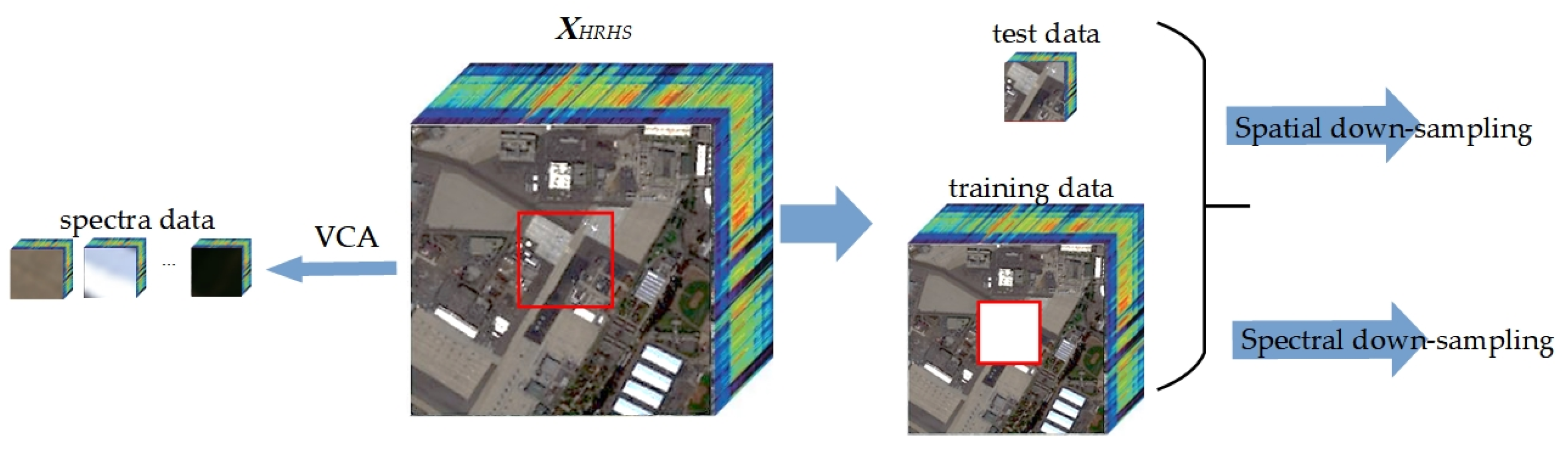
Some state-of-the-art approaches are selected to perform comparative functions, including sparse coding [9], CNMF [32], SSR-NET [33], TFNet [34], and ResTFNet [35]. The sparse coding method aims for RGB image spectral super-resolution with the help of spectral data prior. The remaining methods, CNMF, SSR-NET, TFNet, and ResTFNet, are both designed for multispectral image and hyperspectral image fusion, which can be classified as hyperspectral image-assisted spectral super-resolution. Significantly, the single RGB image super-resolution methods are not within the scope of comparison in this paper, as these methods only focus on the visible spectral range.

3.1. Datasets

In the Section 3, three datasets are utilized to validate the spectral super-resolution performance of the proposed method and comparison algorithms. The detailed introduction of these datasets is as follows:

(1)

San Diego Airport: These data are acquired by the AVIRIS hyperspectral sensor, with a size of 400 × 400 pixels. The spectral range of San Diego Airport data is from 400 nm to 2500 nm. It has 189 valid spectral bands.

(2)

Pavia University: The Pavia University data were obtained by the ROSIS sensor, with a size of 610 × 340 pixels. The spectral range of Pavia University data is from 430 nm to 860 nm, with 103 bands in total. The main ground objects in the Pavia University scene consist of buildings, meadows, Bare Soil, and so on.

(3)

XiongAn [34]: The XiongAn dataset was acquired using a full-spectrum multi-modal imaging spectrometer. The spectral range is from 400 nm to 1000 nm with 250 bands in total. The spatial resolution of this scene is 0.5 m with a size of 3750 × 1580 pixels.

3.2. Evaluation Metrics

To verify the spectral super-resolution effectiveness of the proposed method and comparison methods intuitively, we adopt five commonly used indices, including RMSE, PSNR, ERGAS, SAM, and SSIM. The specific calculation formulas of them are listed as follows.

(1)

Root mean square error (RMSE). RMSE is a direct quantitative evaluation index and it measures reconstructed error by calculating pixel value differences between reference and reconstructed images directly. It can be written as follows:

$$RMSE=\frac{1}{MN}{\sqrt{{\displaystyle \sum _{i=1}^M{\displaystyle \sum _{j=1}^N\left[x\left(i,j,k\right)-\tilde{x}\left(i,j,k\right)\right]}}}}^2,$$

(22)

where M, N, and L are the width, height, and band number of HRHS images, respectively; $x(i,j,k)$ and $\tilde{x}(i,j,k)$ denote pixel value in reference and reconstructed images, respectively.

(2)

Peak signal-to-noise ratio (PSNR). The PSNR of a single spectral band is defined in the following equation. The final PSNR value is calculated by averaging the PSNRs of all bands.

$$PSNR=10{\log }_{10}\left(\frac{\max {\left[x\left(i,j,k\right)\right]}^2}{\frac{1}{MN}\Vert x\left(i,j,k\right)-\tilde{x}\left(i,j,k\right){\Vert }^2}\right),$$

(23)

where $\mathrm{m}\mathrm{a}\mathrm{x}\hspace{0.17em}(·)$ represents the maximum function.

(3)

Relative dimensionless global error in synthesis (ERGAS). ERGAS reflects the image quality of an entire image. The smaller the value, the better the reconstructed effect. The equation of ERGAS is defined as follows:

$$ERGAS=\frac{100}{r}\sqrt{\frac{1}{L}{\displaystyle \sum _{k=1}^L\frac{\Vert x\left(i,j,k\right)-\tilde{x}\left(i,j,k\right){\Vert }^2}{{\left[mean\left(x\left(i,j,k\right)\right)\right]}^2}}},$$

(24)

where r represents the spatial resolution ratio between hyperspectral images and HRHS images; $mean(·)$ denotes the average function.

(4)

Spectral angle mapping (SAM). The SAM index measures the average spectral similarity between reference and reconstructed images, and it is defined as follows:

$$SAM=\frac{1}{MN}\arccos \left[\left({\displaystyle \sum _{q=1}^{MN}x\left(i,j,k\right)*\tilde{x}\left(i,j,k\right)}\right)/\left(\Vert x\left(i,j,k\right)\Vert *\Vert \tilde{x}\left(i,j,k\right)\Vert \right)\right].$$

(25)

(5)

Structural similarity (SSIM). SSIM is a typical metric indicating the similarity of an entire image. The best value of SSIM is 1. The closer to 1, the more similar the two images are. The SSIM is defined as follows:

$$SSIM=\frac{\left(2{\mu }_x{\mu }_{\tilde{x}}+C_1\right)\left(2{\sigma }_{x\tilde{x}}+C_2\right)}{\left({\mu }_x^2+{\mu }_{\tilde{x}}+C_1\right)\left({\sigma }_x^2+{{\sigma }_{\tilde{x}}}^2+C_2\right)},$$

(26)

where ${\mu }_x$ and ${\mu }_{\tilde{x}}$ represent the mean of the reference and reconstructed images, respectively; ${\sigma }_x$ and ${\sigma }_{\tilde{x}}$ represent the standard deviation of the reference and reconstructed images, respectively; ${\sigma }_{x\tilde{x}}$ represents covariance between the reference and reconstructed images; $C_1$ and $C_2$ are constants used for adjustment.

3.3. Network Settings

To simulate the data to be processed, a frequently used endmember extraction method VCA is used to extract hyperspectral point data from the original data. The RGB image is generated by extracting three spectral bands from an HRHS image in the visible range. The center wavelength of the extracted three bands needs to fall within the blue, green, and red band ranges, respectively. For image and image fusion methods, the low-spatial-resolution hyperspectral image is obtained by blurring the HRHS image first and then down-sampling four times. The data simulation process is shown in Figure 3.

For the San Diego Airport dataset, a subarea with a size of 128 × 128 pixels is cropped as the test image. The remaining area is utilized for training purposes. For the Pavia University scene, an area with a size of 128 × 128 pixels is selected as test data, and the remaining image is used for training purposes. For the XiongAn scene, an area with a size of 512 × 512 pixels is selected as test data, and the remaining image is used for training purposes. The number of a priori hyperspectral spectra is set to 150, 100, and 150 in the three datasets, respectively. The number of spectra setting considers both spectral data completeness and network computation complexity. The spectral data are extracted from the original datasets by the VCA algorithm.

In all three datasets, the learning rate is set to 0.0001. The iterations of the gradient descent and soft-threshold operation modules are set to 10. The entire training epoch number is set to 10,000. The learning rate and training epoch number of SSR-NET, TFNet, and ResTFNet are both set to the same as GRSS-Net.

All experiments are conducted on a computer with an Intel Core i9-10900K CPU, with 3.70 Hz and 64 GB RAM. The deep learning-based algorithms are implemented using Pytorch 1.3.0 on Python 3.7.

For the loss function setting, the GRSS-Net adopts the L1 loss function. The other algorithms continue to use the loss function used when they were proposed.

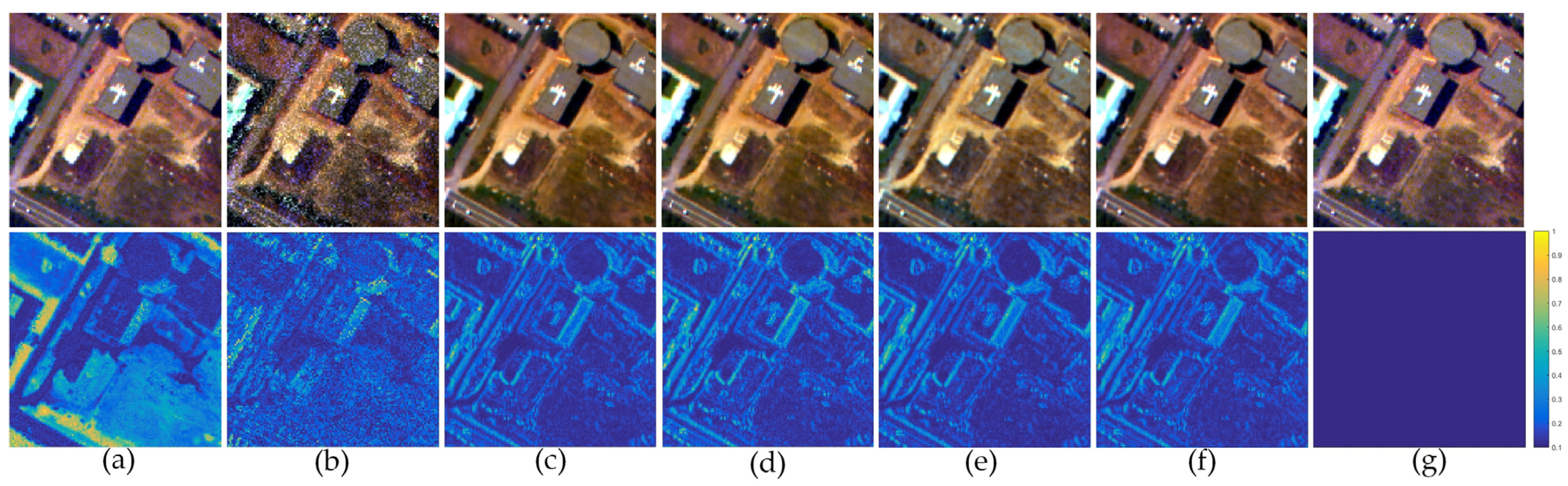
3.4. Quantitative Evaluation

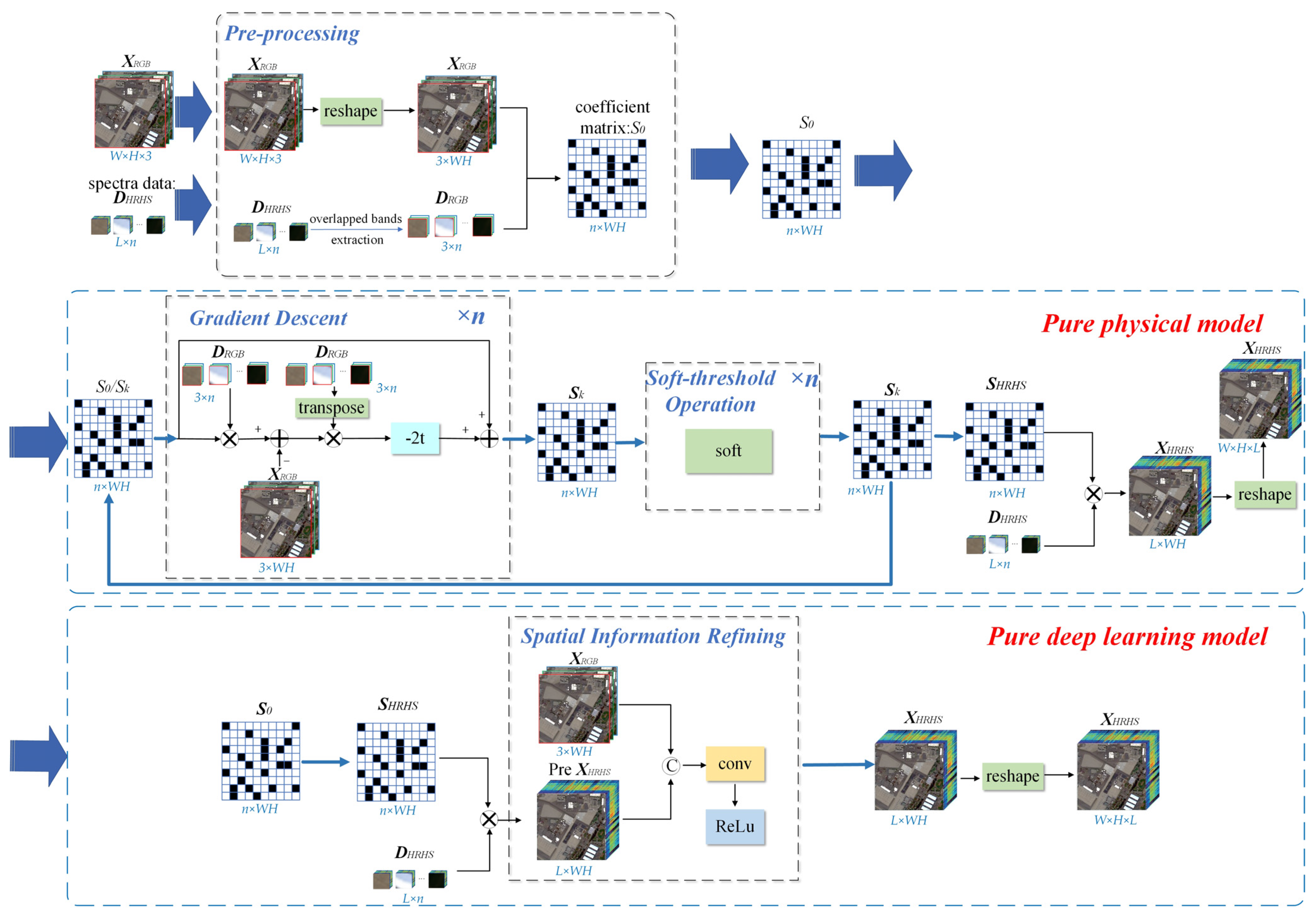
The quantitative evaluation results of these six methods implemented on San Diego Airport data are shown in

Table 2. The fusion evaluation results of six algorithms on San Diego Airport data.

	RMSE (↓,0)	PSNR (↑,+∞)	ERGAS (↓,0)	SAM (↓,0)	SSIM (↑,1)
Sparse coding	23.720	41.034	7.674	10.850	0.775
CNMF	29.553	37.232	5.796	6.170	0.769
TFNet	1.043	47.796	1.546	2.445	0.883
ResTFNet	0.952	47.587	1.398	2.196	0.953
SSR-NET	1.075	47.532	1.590	2.507	0.945
GRSS-Net	1.299	46.889	1.912	3.318	0.962

. In Table 2, the optimal values and the optimal direction of values convergence of five evaluation indicators are shown in parentheses immediately after the indicator name. Meanwhile, the optimal value among six algorithms for each indicator is shown in bold. The markings in the remaining tables of this paper are consistent with Table 2. As depicted, GRSS-Net performs better than the other algorithms at SSIM. It indicates that the proposed method can maintain a better overall image structure during six algorithms on San Diego Airport data. The ResTFNet achieves the most at RMSE, ERGAS, and SAM indicators. For PSNR, the TFNet is better than the other approaches. From the perspective of spectral information fidelity, the ResTFNet method is the best. Overall, the deep learning-based method generally performs better than the traditional physical model-based method. Taking the lack of hyperspectral spatial information into account, the GRSS-Net can almost achieve a fusion effect better than multispectral and hyperspectral image fusion methods. The above-mentioned advantages bring great convenience to the practical application scene. For example, the multispectral and hyperspectral image fusion methods put forward higher requirements for image registration, which is difficult for both satellite data and ground acquisition data. The GRSS-Net can tackle such situations better than traditional pure deep learning-based methods.

The fusion images of six algorithms implemented on the San Diego Airport scene are displayed in Figure 4. As displayed, the first row in Figure 4 is the real RGB synthesis of different fusion results. Considering deep learning-based methods only test on small areas, the traditional physical model-based methods also crop the corresponding area for comparison purposes. The second row shows fusion error images of six fusion images on the basis of the reference image. The color bar for error value reference is shown at the far right of the second row. The yellower the color, the greater the error in the fused image. On the contrary, the bluer the color, the smaller the fusion image error. The fused image of sparse coding shows that sparse coding maintains great spatial information but does not reconstruct spectral information well. The sparse coding algorithm is a typical spectral super-resolution method with prior knowledge of spectral data. However, the feature extraction ability of pure physical models is limited, which leads to spectral information of spectral data and spatial information of RGB images not fusing very well. As a result, the fused result of sparse coding is not ideal. The CNMF algorithm also cannot adapt well to fusion tasks in which the spectral range is not coincident. In contrast, deep learning-based algorithms can handle this application scenario well. It can be found that the fused images of the deep learning-based algorithms perform well in preserving spatial texture information and reconstructing spectral information.

The quantitative evaluation results of six algorithms on Pavia University data are shown in

Table 3. The fusion evaluation results of six algorithms on Pavia University data.

	RMSE (↓,0)	PSNR (↑,+∞)	ERGAS (↓,0)	SAM (↓,0)	SSIM (↑,1)
Sparse coding	12.245	33.969	7.131	6.577	0.702
CNMF	10.202	32.707	6.229	5.625	0.779
TFNet	2.831	38.112	1.957	2.643	0.989
ResTFNet	2.967	38.404	2.106	2.586	0.990
SSR-NET	3.999	36.810	2.709	3.253	0.983
GRSS-Net	3.558	38.674	3.186	3.385	0.982

. As can be seen, the ResTFNet obtains the greatest value of SAM and SSIM, TFNet achieves better in the RMSE and ERGAS indicators, and GRSS-Net achieves better in PSNR than the other algorithms. Similar to the first data, the sparse coding and CNMF methods did not show an ideal image spatial–spectral feature fusion ability. The five indicators of sparse coding and CNMF are at the bottom of the six algorithms. On the other hand, the ground objects in the Pavia University scene are simpler than those in the San Diego Airport scene. Thus, the difference in evaluation indicators between physical model-based methods and deep learning methods is not very significant. For Pavia University data, the deep learning methods achieve great fusion performance.

The fused results of six algorithms implemented on the Pavia University scene are depicted in Figure 5. It can be found that the fusion result of the sparse coding method has a large error in the vegetation coverage area. Consider that this phenomenon may be caused by the complex plant spectral curves and the non-overlapped spectral range not being able to recover accurately. The image fused by the CNMF algorithm has salt-and-pepper noise, which indicates that CNMF cannot resist noise well. For deep learning-based methods, it can be observed that the fusion results of TFNet, ResTFNet, and SSR-NET show a slight hue change compared with the reference image. On the contrary, the fused image of GRSS-Net is more coincident with the reference image.

As depicted, the quantitative evaluation results of the six algorithms on XiongAn data are shown in

Table 4. The fusion evaluation results of six algorithms on XiongAn data.

	RMSE (↓,0)	PSNR (↑,+∞)	ERGAS (↓,0)	SAM (↓,0)	SSIM (↑,1)
Sparse coding	9.245	31.834	6.928	3.183	0.773
CNMF	8.638	33.670	6.318	2.882	0.820
TFNet	2.238	38.474	1.413	2.672	0.996
ResTFNet	2.588	37.213	1.584	2.554	0.995
SSR-NET	2.783	36.583	1.982	2.968	0.989
GRSS-Net	3.091	35.671	2.772	2.501	0.980

. From Table 4, it can be found that the TFNet algorithm achieves the best value in four indicators except for SAM, and the SAM value of ResTFNet is higher than the other methods. The ground objects of the XiongAn scene are relatively simple, including vegetation and bare soil. Such a scenario is friendly for both physical model-based and deep learning-based methods. Therefore, the quantitative evaluation gap between physical model-based methods and deep learning-based methods is not significant compared to the other two images. However, GRSS-Net performs worse than TFNet and ResTFNet on quantitative evaluation, which may be caused by the absence of spatial information in hyperspectral data. But overall, their fusion effect is still at the same level.

The experimental results of the six algorithms on XiongAn data are shown in Figure 6. From the first row, it can be observed that there exists little difference among the six images. Only in the middle of the upper images, which show bare soil, do TFNet and ResTFNet have a slight color shift compared to the reference image. For error images, there exists a large gap. As we can see in the second row, the greatest error of the sparse coding fused image is located in a place with dense vegetation. For the remaining five methods, the major area with high fusion error is located in vegetation shadows, which can be found in the yellow-colored bar area in the second row of Figure 6b–f. Extracting effective information from shadowed areas has always been a challenge because the reflection information in shadowed areas is weaker than in other areas. Thus, how to solve shadowed area fusion still needs further research. Overall, the deep learning-based methods have better fusion quality than traditional physical model-based methods.

3.5. Ablation Study

To verify the effectiveness of combining physical models and deep learning models, a series of ablation studies of GRSS-Net is designed. Two contrasted models are set for comparative purposes. They are a pure physical model and a pure deep learning model. The pure physical model is generated by removing all deep learning layers from GRSS-Net. By contrast, the pure deep learning model is produced by removing the gradient descent and soft-threshold operation modules, which are derived from the physical model. An illustration of the pure physical model and the pure deep learning model is depicted in Figure 7.

These two models and the entire GRSS-Net are implemented on San Diego Airport data, respectively. A quantitative evaluation of the fusion results is displayed in

Table 5. The fusion evaluation results of three models on San Diego Airport data.

	RMSE (↓,0)	PSNR (↑,+∞)	ERGAS (↓,0)	SAM (↓,0)	SSIM (↑,1)
Pure physical model	6.558	31.828	9.601	8.006	0.929
Pure deep learning model	8.354	27.259	11.956	12.289	0.773
GRSS-Net	1.299	45.889	1.912	3.318	0.962

.

As can be seen in Table 5, the entire GRSS-Net achieves a better fusion performance than the other two models on all five evaluation indicators. Another interesting phenomenon that can be found in Table 5 is that the pure deep learning model performs worse than the pure physical model. The main reason is that the original hyperspectral point data do not carry any spatial information, resulting in inaccurate determination of the position where spectral information is injected into RGB images. As a result, it fails to reconstruct spectral information successfully. For the pure physical model-based method, it also does not fuse well because of the loss of effective assistance of deep learning layers. The intuitive fusion results of the three models are illustrated in Figure 8.

As shown in Figure 8, the fusion image of the pure physical model is more blurry than the other images. This proves that the spatial information-refining module can improve spatial reconstruction accuracy effectively. In Figure 8, the fusion results of the pure physical and the pure deep learning model both have color distortion to some extent compared with the fusion result of GRSS-Net and the reference image. The above-mentioned analysis indicates that the combined model can acquire better fusion performance than a single model.

4. Discussion

4.1. Effect Validation in Spatial Misalignment Scenes

The matching of hyperspectral data with overlapped or partially overlapped spatial scenes of RGB is a vital requirement in most methods. However, due to various restrictive reasons, it is not always possible to obtain hyperspectral data within the same spatial range in actual RGB super-resolution application situations.

The proposed GRSS-Net has small restrictions on hyperspectral data-obtaining scenarios, as long as the hyperspectral data cover the majority of ground objects in an RGB image scene. Thus, GRSS-Net does not require image registration or other types of spatial dimension processing, making it superior to other methods. In the following content, a series of experiments is designed to further verify this point.

The three datasets mentioned In Section 3.1 are further processed to be implemented in this set of experiments. For all data, the spectral data extraction area is entirely different from the area of simulated RGB (as depicted in Figure 9).

The true color synthesis images of the spatial dislocation experimental results of three datasets are exhibited in Figure 10. As clearly displayed in Figure 10, the fusion error images achieve a fine performance on all three datasets. The hue of the fused results is roughly the same as the reference images. This conclusion is consistent with the conclusion drawn in Section 3.4.

The quantitative evaluation results of the spatial dislocation experiments on three datasets are shown in

Table 6. The fusion evaluation results of spatial misalignment experiments.

	RMSE (↓,0)	PSNR (↑,+∞)	ERGAS (↓,0)	SAM (↓,0)	SSIM (↑,1)
San Diego Airport	1.355	46.279	2.012	3.348	0.952
Pavia University	3.719	38.441	2.417	3.172	0.978
XiongAn	3.185	35.637	2.648	2.483	0.974

. As depicted in Table 6, a conclusion can be drawn that there is no significant difference between the quantitative results of GRSS-Net on three datasets in spatial dislocation experiments and the general experiments shown in Section 3.4. This phenomenon indicates that the proposed GRSS-Net can achieve the same fusion effect regardless of whether the spectral data are in the same region as the RGB image. The above analysis further proves that the GRSS-Net has fewer requirements for assisted hyperspectral data compared with other methods. Therefore, GRSS-Net can be utilized in scenes where there are no strictly matched hyperspectral data. In this situation, some hyperspectral images with similar ground objects or spectral data collected using PSR or ASD can fill in the gaps.

4.2. Validation Experiments on ZY1E Images

In order to evaluate the spectral reconstruction performance in actual application scenes, a pair of ZY1E images are selected to implement GRSS-Net. This group of data includes an RGB image with a size of 512 × 512 pixels and an HSI image with a size of 400 × 400 pixels. The RGB image is simulated from an original multispectral image by extracting RGB bands. The spectral range of HSI in the ZY1E scene is from 396 nm to 1040 nm, with 76 bands in total. The spatial resolution of the RGB image and the HSI image are 10 m and 30 m, respectively. The images’ acquisition date is 29 July 2021. The RGB image, true color synthesis HSI image, and standard false color synthesis HSI image are displayed in Figure 11a–c, respectively.

The HSI image is utilized to train the model used in this experiment. The training data are simulated in the way mentioned in Section 3.3. After obtaining the trained model, an RGB image is put into the model to generate an HRHS image. The final generated HRHS image is shown in Figure 12. Due to the lack of a real reference HRHS image, there is no quantitative evaluation in this experiment.

As shown in Figure 11a,b, the main ground objects in this scene are vegetation and soil. Therefore, whether the red-edge information can be accurately reconstructed is an important criterion for measuring whether the spectral information is accurately reconstructed in this scene. The standard false color synthesis of the result can reflect red-edge information to some extent. It can be found that Figure 12b has the same hue as Figure 11c. This phenomenon indicates that the red-edge information in the ZY1E scene is well reconstructed using GRSS-Net.

5. Conclusions

To solve the problem of difficult hyperspectral image acquisition, spectral super-resolution methods have emerged. At present, spectral super-resolution methods consist of two main categories, including traditional physical model-based methods and deep learning-based methods. The traditional physical model-based methods have an identical and clear physical meaning but their feature extraction ability is insufficient. The deep learning-based methods have powerful feature extraction capability but lack physical explanation, leading to poor transferability. From the perspective of whether prior hyperspectral data are needed, it also can be divided into pure RGB image spectral super-resolution methods and spectral super-resolution methods needing prior hyperspectral data. The spectral reconstruction range of pure RGB image spectral super-resolution methods is limited to the visible spectral range. In contrast, spectral super-resolution methods needing prior hyperspectral data can handle spectral-resolution problems with a wider spectral range.

Taking the above analysis into consideration, a generally interpretable deep network for RGB image spectral super-resolution is proposed, abbreviated as GRSS-Net, which needs hyperspectral point data as prior knowledge. The proposed GRSS-Net takes compressed sensing as an underlying principle, depending on the non-linear feature extraction ability of deep learning layers, then integrates them into a complete deep learning network architecture. This way, the GRSS-Net has the following advantages: (1) It can handle various spectral super-resolution scenes with different spectral ranges; (2) It has both a clear physical meaning and great feature extraction ability; (3) It enables deep learning frameworks to handle point–surface fusion problems with the help of traditional physical models; (4) Since GRSS-Net does not require hyperspectral images as auxiliary data, it does not need to consider image registration issues compared with two image fusion scenes. In addition, the prior hyperspectral point data can be acquired from hyperspectral images with the same ground objects or spectral data obtained by a portable spectrometer. A series of comparative experiments proved that the proposed GRSS-Net can achieve an effect comparable to the deep learning methods which need hyperspectral images as auxiliary data. In practical application scenarios, the optimization method, the basic image observation model, and the deep learning-based module in GRSS-Net can be replaced flexibly according to different application tasks to improve the actual super-resolution effectiveness.

References

1. Yokoya, N.; Grohnfeldt, C.; Chanussot, J. Hyperspectral and Multispectral Data Fusion: A comparative review of the recent literature. IEEE Geosci. Remote Sens. Mag. 2017, 5, 29–56. [Google Scholar] [CrossRef]
2. Farzaneh, D.; Farhad, S.; Soroosh, M.; Ahmad, T.; Reza, K.; Alfred, S. A review of image fusion techniques for pan-sharpening of high-resolution satellite imagery. ISPRS J. Photogramm. 2021, 171, 101–117. [Google Scholar]
3. Hong, D.; Han, Z.; Yao, J.; Gao, L.; Zhang, B.; Plaza, A.; Chanussot, J. SpectralFormer: Rethinking Hyperspectral Image Classification With Transformers. IEEE Trans. Geosci. Remote Sens. 2022, 60, 5518615. [Google Scholar] [CrossRef]
4. Qi, W.; Huang, C.; Wang, Y.; Zhang, X.; Sun, W.; Zhang, L. Global-Local Three-Dimensional Convolutional Transformer Network for Hyperspectral Image Classification. IEEE Trans. Geosci. Remote Sens. 2023, 61, 5510820. [Google Scholar] [CrossRef]
5. Zhang, Y.; Fan, Y.; Xu, M.; Li, W.; Zhang, G.; Liu, L.; Yu, D. An Improved Low Rank and Sparse Matrix Decomposition-Based Anomaly Target Detection Algorithm for Hyperspectral Imagery. IEEE J. Sel. Top. Appl. Earth Observ. Remote Sens. 2020, 13, 2663–2672. [Google Scholar] [CrossRef]
6. Zhang, H.; Xu, H.; Tian, X.; Jiang, J.; Ma, J. Image fusion meets deep learning: A survey and perspective. Inform. Fusion 2021, 76, 323–336. [Google Scholar] [CrossRef]
7. Han, X.; Yu, J.; Xue, J.H.; Sun, W. Hyperspectral and Multispectral Image Fusion Using Optimized Twin Dictionaries. IEEE Trans. Image Process. 2020, 29, 4709–4720. [Google Scholar] [CrossRef]
8. Xie, Q.; Zhou, M.; Zhao, Q.; Xu, Z.; Meng, D. MHF-Net: An Interpretable Deep Network for Multispectral and Hyperspectral Image Fusion. IEEE Trans. Pattern Anal. Mach. Intell. 2020, 44, 1457–1473. [Google Scholar] [CrossRef]
9. Arad, B.; Ben Shahar, O. Sparse Recovery of Hyperspectral Signal from Natural RGB Images. In Proceedings of the European Conference on Computer Vision, Amsterdam, The Netherlands, 8–10 and 15–16 October 2016. [Google Scholar]
10. Hu, J.; Huang, T.; Deng, L.; Dou, H.; Hong, D.; Vivone, G. Fusformer: A Transformer-Based Fusion Network for Hyperspectral Image Super-Resolution. IEEE Geosci. Remote Sens. Lett. 2022, 19, 6012305. [Google Scholar] [CrossRef]
11. Jia, S.; Min, Z.; Fu, X. Multiscale spatial–spectral transformer network for hyperspectral and multispectral image fusion. Inform. Fusion 2023, 96, 117–129. [Google Scholar] [CrossRef]
12. Li, S.; Dian, R.; Liu, B. Learning the external and internal priors for multispectral and hyperspectral image fusion. Sci. China Inform. Sci. 2022, 66, 140303. [Google Scholar] [CrossRef]
13. Dian, R.; Li, S.; Sun, B.; Guo, A. Recent advances and new guidelines on hyperspectral and multispectral image fusion. Inform. Fusion 2021, 69, 40–51. [Google Scholar] [CrossRef]
14. Wei, Q.; Bioucas-Dias, J.; Dobigeon, N.; Tourneret, J.Y. Hyperspectral and Multispectral Image Fusion based on a Sparse Representation. IEEE Trans. Geosci. Remote Sens. 2015, 53, 3658–3668. [Google Scholar] [CrossRef]
15. Cheng, J.; Liu, H.J.; Liu, T.; Wang, F.; Li, H.S. Remote sensing image fusion via wavelet transform and sparse representation. ISPRS J. Photogramm. 2015, 104, 158–173. [Google Scholar] [CrossRef]
16. Deng, S.; Deng, L.; Wu, X.; Ran, R.; Hong, D.; Vivone, G. PSRT: Pyramid Shuffle-and-Reshuffle Transformer for Multispectral and Hyperspectral Image Fusion. IEEE Trans. Geosci. Remote Sens. 2023, 61, 5503715. [Google Scholar] [CrossRef]
17. Liu, Z.; Zheng, Y.; Han, X.H. Deep Unsupervised Fusion Learning for Hyperspectral Image Super Resolution. Sensors 2021, 21, 2348. [Google Scholar] [CrossRef] [PubMed]
18. Zhu, Z.; Liu, H.; Hou, J.; Jia, S.; Zhang, Q. Deep Amended Gradient Descent for Efficient Spectral Reconstruction From Single RGB Images. IEEE Trans. Comput. Imaging 2021, 7, 1176–1188. [Google Scholar] [CrossRef]
19. Vivone, G. Multispectral and hyperspectral image fusion in remote sensing: A survey. Inform. Fusion 2023, 89, 405–417. [Google Scholar] [CrossRef]
20. Li, J.; Hong, D.; Gao, L.; Yao, J.; Zheng, K.; Zhang, B.; Chanussot, J. Deep learning in multimodal remote sensing data fusion: A comprehensive review. Int. J. Appl. Earth Obs. Geoinf. 2022, 112, 102926. [Google Scholar] [CrossRef]
21. Peng, Y. Blind Fusion of Hyperspectral Multispectral Images Based on Matrix Factorization. Remote Sens. 2021, 13, 4219. [Google Scholar]
22. Guo, H.; Bao, W.X.; Feng, W.; Sun, S.S.; Mo, C.; Qu, K. Multispectral and Hyperspectral Image Fusion Based on Joint-Structured Sparse Block-Term Tensor Decomposition. Remote Sens. 2023, 15, 4610. [Google Scholar] [CrossRef]
23. Hang, R.; Liu, Q.; Li, Z. Spectral Super-Resolution Network Guided by Intrinsic Properties of Hyperspectral Imagery. IEEE Trans. Image Process. 2021, 30, 7256–7265. [Google Scholar] [CrossRef] [PubMed]
24. Li, J.; Li, Y.; Wang, C.; Ye, X.; Heidrich, W. BUSIFusion: Blind Unsupervised Single Image Fusion of Hyperspectral and RGB Images. IEEE Trans. Comput. Imaging 2023, 9, 94–105. [Google Scholar] [CrossRef]
25. Gao, L.; Hong, D.; Yao, J.; Zhang, B.; Gamba, P.; Chanussot, J. Spectral Superresolution of Multispectral Imagery with Joint Sparse and Low-Rank Learning. IEEE Trans. Geosci. Remote Sens. 2021, 59, 2269–2280. [Google Scholar] [CrossRef]
26. Selesnick, I.W. Sparse Signal Restoration. Connexions Web Site. 2009. Available online: http://cnx.org/content/m32168/1.3/contentinfo (accessed on 28 April 2019).
27. Liang, D.; Liu, B.; Wang, J.; Ying, L. Accelerating Sense Using Compressed Sensing. Magn. Reson. Med. 2009, 62, 1574–1584. [Google Scholar] [CrossRef]
28. Sun, T.; Tang, K.; Li, D. Gradient Descent Learning with Floats. IEEE Trans. Cybern. 2022, 52, 1763–1771. [Google Scholar] [CrossRef]
29. Beck, A.; Teboulle, M. A Fast Iterative Shrinkage-Thresholding Algorithm for Linear Inverse Problems. Siam J. Imaging Sci. 2009, 2, 183–202. [Google Scholar] [CrossRef]
30. Zhang, J.; Ghanem, B. ISTA-Net: Interpretable Optimization-Inspired Deep Network for Image Compressive Sensing. In Proceedings of the 2018 IEEE/CVF Conference on Computer Vision and Pattern Recognition, Wellington, New Zealand, 14–16 December 2018. [Google Scholar]
31. Olshausen, B.A.; Field, D.J. Emergence of simple-cell receptive fieldproperties by learning a sparse code for natural images. Nature 1996, 381, 607–609. [Google Scholar] [CrossRef]
32. Yokoya, N.; Yairi, T.; Iwasaki, A. Coupled Nonnegative Matrix Factorization Unmixing for Hyperspectral and Multispectral Data Fusion. IEEE Trans. Geosci. Remote Sens. 2012, 50, 528–537. [Google Scholar] [CrossRef]
33. Zhang, X.T.; Huang, W.; Wang, Q.; Li, X.L. SSR-NET: SpatialSpectral Reconstruction Network for Hyperspectral and Multispectral Image Fusion. IEEE Trans. Geosci. Remote Sens. 2021, 59, 5953–5965. [Google Scholar] [CrossRef]
34. Liu, X.; Liu, Q.; Wang, Y. Remote sensing image fusion based on two-stream fusion network. Inform. Fusion 2020, 55, 1–15. [Google Scholar] [CrossRef]
35. Cen, Y.; Zhang, L.; Zhang, X.; Wang, Y.; Qi, W.; Tang, S.; Zhang, P. Aerial hyperspectral remote sensing classification dataset of Xiongan New Area (Matiwan Village). J. Remote Sens. 2020, 24, 1299–1306. [Google Scholar]
Figure 1. The illustration of the observation model in proposed method.
Remotesensing 16 00139 g001
Figure 2. The flowchart of proposed architecture.
Remotesensing 16 00139 g002
Figure 3. The flowchart of data simulation.
Remotesensing 16 00139 g003
Figure 4. Fusion results of six algorithms on San Diego Airport data. The first row displays the real RGB synthesis (29-13-4 bands) of San Diego Airport data. The second row shows the fusion error between fusion results and the ground truth image: (a) Sparse coding; (b) CNMF; (c) TFNet; (d) ResTFNet; (e) SSR-NET; (f) GRSS-Net; (g) Reference.
Remotesensing 16 00139 g004
Figure 5. Fusion results of six algorithms on Pavia University data. The first row displays the real RGB synthesis (67-29-1 bands) of Pavia University data. The second row shows the fusion error between fusion results and the ground truth image: (a) Sparse coding; (b) CNMF; (c) TFNet; (d) ResTFNet; (e) SSR-NET; (f) GRSS-Net; (g) Reference.
Remotesensing 16 00139 g005
Figure 6. Fusion results of six algorithms on XiongAn data. The first row displays the real RGB synthesis (120-72-36 bands) of different fusion results on XiongAn data. The second row shows the fusion error between fusion results and the ground truth image: (a) Sparse coding; (b) CNMF; (c) TFNet; (d) ResTFNet; (e) SSR-NET; (f) GRSS-Net; (g) Reference.
Remotesensing 16 00139 g006
Figure 7. The illustration of pure physical model and pure deep learning model.
Remotesensing 16 00139 g007
Figure 8. Fusion results of three models using San Diego Airport data. The first row displays the real RGB synthesis (29-13-4 bands) of different fusion results on San Diego Airport data. The second row shows the fusion error between fusion results and the ground truth image: (a) Pure physical model; (b) Pure deep learning model; (c) GRSS-Net; (d) Reference.
Remotesensing 16 00139 g008
Figure 9. The flowchart of data simulation in spatial misalignment experiments.
Remotesensing 16 00139 g009
Figure 10. Fusion results of spatial misalignment experiments on three datasets: (a) fusion results of San Diego Airport data; (b) reference images of San Diego Airport data; (c) fusion results of Pavia University data; (d) reference images of Pavia University data; (e) fusion results of XiongAn data; (f) reference images of XiongAn data.
Remotesensing 16 00139 g010
Figure 11. The true color synthesis of (a) RGB image, and (b) HSI image of ZY1E data. The standard false color synthesis of (c) HSI image of ZY1E data.
Remotesensing 16 00139 g011
Figure 12. The (a) true color synthesis and (b) standard false color synthesis of result.
Remotesensing 16 00139 g012