Feature Selection for Edge Detection in PolSAR Images

Abstract

Edge detection is one of the most critical operations for moving from data to information. Finding edges between objects is relevant for image understanding, classification, segmentation, and change detection, among other applications. The Gambini Algorithm is a good choice for finding evidence of edges. It finds the point at which a function of the difference of properties is maximized. This algorithm is very general and accepts many types of objective functions. We use an objective function built with likelihoods. Imaging with active microwave sensors has a revolutionary role in remote sensing. This technology has the potential to provide high-resolution images regardless of the Sun’s illumination and almost independently of the atmospheric conditions. Images from PolSAR sensors are sensitive to the target’s dielectric properties and structures in several polarization states of the electromagnetic waves. Edge detection in polarimetric synthetic-aperture radar (PolSAR) imagery is challenging because of the low signal-to-noise ratio and the data format (complex matrices). There are several known marginal models stemming from the complex Wishart model for the full complex format. Each of these models renders a different likelihood. This work generalizes previous studies by incorporating the ratio of intensities as evidence for edge detection. We discuss solutions for the often challenging problem of parameter estimation. We propose a technique which rejects edge estimates built with thin evidence. Using this idea of discarding potentially irrelevant evidence, we propose a technique for fusing edge pieces of evidence from different channels that only incorporate those likely to contribute positively. We use this approach for both edge and change detection in single- and multilook images from three different sensors.

1. Introduction

Blake and Isard [1], among others, stressed the importance of prior knowledge in image processing and machine vision for a wide range of application domains. Such knowledge can be posed in several ways, being ”edge” basilar elements. An edge establishes a discontinuity in the image data properties, usually intensity. Most computer vision algorithms assume that edges occur at positions with rapid intensity or color variation [2]. Such an assumption is, at best, misleading when using synthetic-aperture radar (SAR) imagery for two reasons. First, SAR images are contaminated by an interference pattern, speckle, which is neither additive nor Gaussian and reduces the signal-to-noise ratio. Second, the usual formats are either scalar (an intensity band), bivariate (two intensity polarizations), or multivariate complex (covariance matrix). None of them can be naturally translated into ”colors”.

Gambini et al. [3] provided a solution: an edge detection algorithm that finds changes between the statistical properties of the interior and exterior of a boundary. The boundary evolves towards a configuration that maximizes such difference. This approach was optimized by Gambini et al. [4] using a line search algorithm: instead of searching for the whole boundary, the authors proposed estimating points and then joining them with a B-spline curve.

The line-search approach proved its usefulness with several estimation criteria: maximum likelihood [5], stochastic distances [6], geodesic distances [7], and nonparametric statistics [8] among them.

Borba et al. [9] exploited the strength of the statistical modeling approaches as described in [4,5,6]. The evidence of the edges was extracted separately from each polarimetric intensity channel using the maximum-likelihood method by employing the Wishart model for PolSAR data, followed by their fusion for final edge extraction. Since the diversity of edge information between the landcover classes (agricultural fields, urban, sea, etc.) was observed to be distributed over the polarimetric channels, it justified the need for fusing the edge evidences for piecewise aggregation of the boundary information.

Rey et al. [10] addressed the demand for monitoring inland and coastal water bodies in the presence of several observational issues like surrounding vegetation and wind. Such issues lead to fuzzy edges, extending the zone of radiometric transition that makes identifying the edge boundary progressively challenging.

This statistical approach to edge detection relies on specifying the data distribution. When using PolSAR data, there are several options, e.g., the full covariance matrix, each of the three intensity channels, pairs of intensity channels, the three intensity channels, ratio of intensities, phase differences, and pairs intensity-phase difference. Previous works did not exploit the last three models.

Change detection is one of the most active and challenging research areas in remote sensing. Change detection techniques aim at identifying relevant natural or manmade alterations using at least two images from the area under study Asokan and Anitha [11] Bouhlel et al. [12] exploited a method to change detection named determinant ratio test (DRT) using the constant false alarm rate (CFAR) to provide a threshold to build a binary change map. See Touzi et al. [13], Schou et al. [14] for details about CFAR methods. Edges can also be used for change detection. Rather than trying to identify changes in pixels, we show the viability of studying the temporal evolution of the edges between regions.

The previous fusion methods employ all the sources of evidence in an unweighted manner. We present a technique based on the statistical receiver operating characteristic information fusion (S-ROC), which we call $\tau$S-ROC, that incorporates the quality of the estimated edge. Furthermore, we propose a change in the Gambini algorithm that solves instability problems. Moreover, we verify the new method’s feasibility for change detection.

This article presents three improvements: two marginal models, the $\tau$S-ROC information fusion, and a decision rule for the Gambini algorithm. Firstly, we add two densities: the ratio of pairs of intensities and the gamma model for the span. Secondly, the $\tau$S-ROC technique truncates the number of PCA components in the information fusion. Thirdly, we enhance the Gambini algorithm with a statistically-based decision rule that may decide not to identify an edge.

This article is structured as follows. Section 2 describes:

(i)

Computational Resources used in this research.

(ii)

The data (images) used in this research.

(iii)

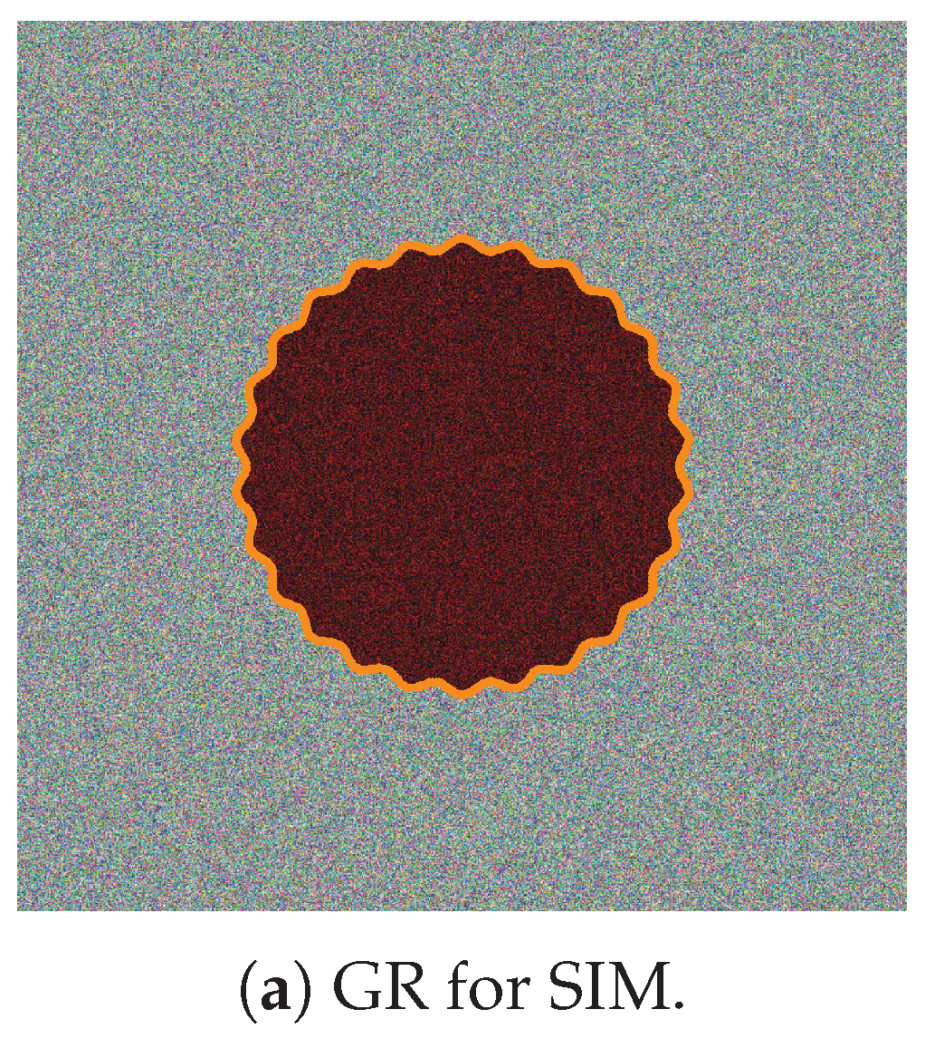
The ground references (GR) for each image.

(iv)

The Gambini algorithm (GA).

(v)

The statistical models stipulated through their probability density functions. In this article, we add two models not used in the literature for edge detection.

(vi)

Information fusion. We propose a new approach named $\tau$S-ROC. We use the principal component analysis (PCA) and a threshold $\tau$ to compute each image’s weight in the fusion process.

(vii)

We conclude this section by discussing the Hausdorff distance (Hd) as a quality measure.

Section 3 presents the results of the methodology proposed when applied to PolSAR data and a new technique to control if a radial line does cross an edge. Section 4 discusses the results, highlighting some positive and negative points, and we present the conclusions in Section 5.

2. Materials and Methods

2.1. Computational Resources

We performed the experiments presented in this work in an Intel© Core i7-9750HQ CPU 2.6 GHz computer with 16 GB of RAM running Debian 11. All the coding was performed using Python 3.9.

2.2. Data

In this work, we use simulated and PolSAR images from sensors:

• The Flower, a simulated image (SIM) produced using the Whishart distribution. Details about this phantom can be found in Gambini et al. [3]; Figure 1a shows a sample along with the true edge between background and foreground.
• Airborne AIRSAR sensor in L-Band data [15]:

  (a)

  The Flevoland (FLEV) dataset from the Netherlands was acquired in August of 1989, and it presented approximately 10 m of resolution (Figure 1b).

  (b)

  The San Francisco (SF) Bay Area in California, USA. The image was acquired in 1989 with the same resolution as the image FLEV (Figure 1c).

• Airborne Uninhabited Aerial Vehicle Synthetic Aperture Radar (UAVSAR) sensor in L-Band available on [16]:

  (a)

  Image of Los Angeles (LAA) acquired on 23 April 2009 (Figure 2a).

  (b)

  Image of Los Angeles (LAM) acquired on 11 May 2015 (Figure 2b).

• OrbiSAR-2 sensor in P-Band image available on [17]:

  (a)

  Sub-scene 01 of Santos City, Brazil (S01) acquired with the airborne OrbiSAR-2 sensor in P-Band (Figure 3a).

  (b)

  Sub-scene 02 of Santos City, Brazil (S02) also acquired with the airborne sensor provides details about the S01 and S02 datasets (Figure 3b). Both images were acquired on 12 August 2015.

2.3. Ground References and Images

The edge in the simulated image (SIM, cf. Figure 1a) is stipulated as an expression in polar coordinates. In this case, the ground reference (GR) is the discrete version of this edge.

We analyzed the images from actual sensors pixel-by-pixel using false-color compositions of intensity bands and Pauli decompositions. We marked all the pixels that separate different classes.

2.4. The Gambini Algorithm

The Gambini algorithm (GA) attempts to find evidence of an edge over a thin data strip. A border between regions with different characteristics along the strip is defined at the position of maximal change of an arbitrary feature. The strength of the GA is demonstrated by its applicability under noisy conditions with any model that describes the data well.

We use the Bresenham line algorithm to extract the strips of pixels on which the GA operates. Moreover, we discard at this stage zero-valued pixels that prevent the computation of ratios and logarithms.

The first version of the GA algorithm [3] was computationally intensive because it required iterating a likelihood function. Nascimento et al. [6] reduced the computational cost by using stochastic distances between the PolSAR samples. Naranjo-Torres et al. [7] employed the geodesic distance between SAR intensity samples to measure the dissimilarity between models. These approaches used statistical models with parameters that describe varying degrees of roughness, a feature that proved essential for edge detection.

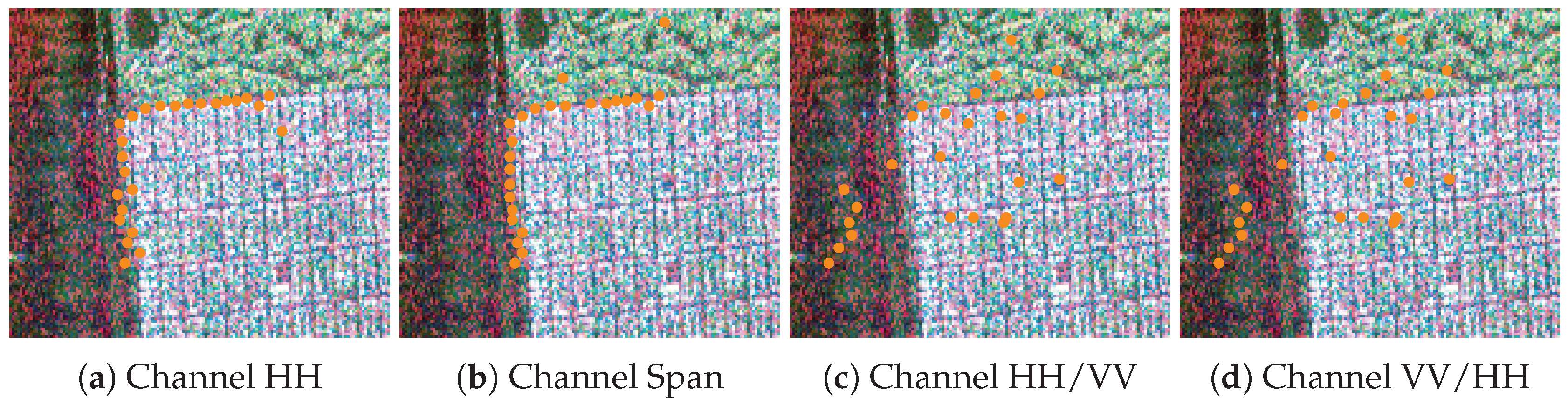
2.5. Distributions

PolSAR systems register the difference between the transmission and reception of amplitude and phase of signals yielding four polarization channels: $S_{\mathrm{HH}}$, $S_{\mathrm{HV}}$, $S_{\mathrm{VH}}$, and $S_{\mathrm{VV}}$ (H for horizontal and V for vertical). If the reciprocity theorem conditions [18] are satisfied, then $S_{\mathrm{HV}}=S_{\mathrm{VH}}$. Defining the single-look scattering vector as

$$\mathbf{S}={\left[\begin{array}{ccc}{S}_{\mathrm{HH}}& S_{\mathrm{HV}}& S_{\mathrm{VV}}\end{array}\right]}^{\mathrm{T}}.$$

(1)

Thus, the scaled multilook PolSAR return has, in each pixel, the form:

$$\mathbf{Z}=\frac{1}{L}\sum _{\ell =1}^L\left[\begin{array}{c}{S}_{\mathrm{HH}}^{(\ell )}\\ S_{\mathrm{HV}}^{(\ell )}\\ S_{\mathrm{VV}}^{(\ell )}\end{array}\right]\left[\begin{array}{ccc}{S}_{\mathrm{HH}}^{*(\ell )}& S_{\mathrm{HV}}^{*(\ell )}& S_{\mathrm{VV}}^{*(\ell )}\end{array}\right],$$

where L is the number of looks, and $S_i$ with $i\in \{\mathrm{HH},\mathrm{HV},\mathrm{VV}\}$ is the scattering in each polarization. The superscript * represents the complex conjugate.

Goodman [19] discussed the properties of the full covariance matrix, and Lee et al. [20] derived several of its marginal distributions. Hagedorn et al. [21] obtained the joint distribution of the three intensity channels.

The Wishart distribution is the accepted model for data in covariance matrix format assuming fully developed speckle. The reader is referred to the work by Ferreira et al. [22] for details and extensions. The probability density function (PDF) that characterizes the Wishart distribution is

$$f_{\mathbf{Z}}(\mathbf{Z};\mathrm{\Sigma },L)=\frac{L^{mL}{\left|\mathbf{Z}\right|}^{L-m}}{{\left|\mathrm{\Sigma }\right|}^L{\mathrm{\Gamma }}_m\left(L\right)}exp(-Ltr\left({\mathrm{\Sigma }}^{-1}\mathbf{Z}\right)),$$

(2)

where $tr\left(·\right)$ is a trace operator, ${\mathrm{\Sigma }}_{m\times m}$ is the complex covariance matrix with entries ${\sigma }_{i,j}$ such that is if $i=j$ then ${\sigma }_{i,j}={\sigma }_i^2$, and ${\mathrm{\Gamma }}_m\left(L\right)$ is the multivariate gamma function defined by:

$${\mathrm{\Gamma }}_m\left(L\right)={\pi }^{\frac{1}{2}m(m-1)}\prod _{i=0}^{m-1}\mathrm{\Gamma }(L-i),$$

(3)

and $\mathrm{\Gamma }\left(·\right)$ is the gamma function. The Wishart distribution describes fully polarimetric data.

In this work, we are interested in the amount of information different marginal components provide for edge detection. To use such components in the GA algorithm, we use the following distributions that stem from the Wishart model:

• Gamma univariate PDF for intensities: the distribution of each intensity channel follows a gamma law with probability density function

  $$f_{\mathbf{Z}}(z;\mu ,L)=\frac{L^L}{\mathrm{\Gamma }\left(L\right){\mu }^L}{z}^{L-1}exp\left\{-\frac{L}{\mu }z\right\}{{\displaystyle \mathrm{𝟙}}}_{{\mathbb{R}}_{+}}\left(z\right),$$

  (4)

  where $L>0$ (rather than $L\ge 1$ to allow for flexibility), $\mu >0$ is the mean, and ${\mathrm{𝟙}}_A$ is the indicator function of the set A. Given the random sample $\mathit{Z}=(Z_1,Z_2\dots ,Z_n)$, its reduced log-likelihood under the Wishart model is

  $$\ell (L,\mu ;\mathit{Z})=n\left[Lln(L/\mu )-ln\mathrm{\Gamma }\left(L\right)\right]+L\sum _{k=1}^{n}ln{Z}_k-\frac{L}{\mu }\sum _{k=1}^n{Z}_k.$$

  (5)
• The density that characterizes the ratio of any pair of intensities is

  $$f(r;\rho ,L)=\frac{\mathrm{\Gamma }\left(2L\right){(1-{\rho }^2)}^L(1+r)r^{L-1}}{\mathrm{\Gamma }\left(L\right)\mathrm{\Gamma }\left(L\right){\left[{(1+r)}^2-4{\rho }^{2}r\right]}^{\frac{2L+1}{2}}}{\mathrm{𝟙}}_{{\mathbb{R}}_{+}}\left(r\right),$$

  (6)

  where $\rho >0$ and $L>0$. We can normalize the ratio of intensities as

  $$r=\frac{{\sum }_{k=1}^n\frac{|S_i{\left(k\right)|}^2}{{\sigma }_i}}{{\sum }_{k=1}^n\frac{|S_j{\left(k\right)|}^2}{{\sigma }_j}}=\frac{{\sum }_{k=1}^n{\left|S_i\left(k\right)\right|}^2}{\tau {\sum }_{k=1}^n{\left|S_j\left(k\right)\right|}^2}.$$

  (7)
  If we define $z=\tau r$, with $\tau ={\sigma }_i/{\sigma }_j$ with $i\in \{\mathrm{HH},\mathrm{HV},\mathrm{VV}\}$ and $i\ne j$, where $\tau$ is the ratio intensity parameter, then (6) becomes

  $$f(z;\rho ,L,\tau )=\frac{{\tau }^L\mathrm{\Gamma }\left(2L\right){(1-{\rho }^2)}^L(\tau +z)z^{L-1}}{\mathrm{\Gamma }\left(L\right)\mathrm{\Gamma }\left(L\right){\left[{(\tau +z)}^2-4\tau {\rho }^{2}z\right]}^{\frac{2L+1}{2}}}.$$

  (8)
  The reduced log-likelihood function under this model is

  $$\begin{array}{c}\ell (\rho ,L,\tau ;\mathit{Z})=n\left(Lln\tau +ln\mathrm{\Gamma }\left(2L\right)+Lln(1-{\rho }^2)-2ln\mathrm{\Gamma }\left(L\right)\right)\hfill \\ \hfill +\sum _{k=1}^{n}ln(\tau +Z_k)+L\sum _{k=1}^{n}ln{Z}_k-\frac{2L+1}{2}\sum _{k=1}^{n}ln\left[{(\tau +Z_k)}^2-4\tau {\rho }^2{Z}_k\right].\end{array}$$

  (9)
• Feng et al. [23] show that the gamma distribution models the span, i.e., the sum of the intensities:

  $$f_{\mathbf{S}}(s;\mu ,L)=\frac{L^L}{\mathrm{\Gamma }\left(L\right){\mu }^L}{s}^{L-1}exp\left\{-\frac{L}{\mu }s\right\}{\mathrm{𝟙}}_{{\mathbb{R}}_{+}}\left(s\right),$$

  (10)

  where $\mu >0$ and $L>0$. The reduced log-likelihood under this model for the random sample $\mathit{S}=(S_1,S_2,\dots ,S_n)$ is:

  $$\ell (\mu ,L;\mathit{S})=n\left[Lln\frac{L}{\mu }-ln\mathrm{\Gamma }\left(L\right)\right]+L\sum _{k=1}^{n}ln{S}_k-\frac{L}{\mu }\sum _{k=1}^n{S}_k.$$

  (11)

We obtain the maximum-likelihood parameter estimates (MLE) by maximizing the reduced log-likelihood function with the Broyden–Fletcher–Goldfarb–Shanno (BFGS) method [24]. It is necessary to provide an initial point to optimize the log-likelihood functions. After finding the parameters, we build the total log-likelihood of the data strip and find the edge evidence by applying the generalized simulated annealing (GenSA) [25] method. The log-likelihood total is non-differentiable and oscillates at the extremities of its domain. The GenSA solves the first problem. The second problem was solved by defining a data slack at the extremities. For more details, see Borba et al. [9].

2.6. Information Fusion Methods

Borba et al. [9] discussed the fusion of the detected edge evidence in each intensity channel of a PolSAR image. Based on these ideas, we propose to include the ratio of intensities and the span. We use the principal components analysis (PCA) based method because it can indicate the relative weights of the channels, thus allowing us to decide whether to use or not each data layer.

The edge information from selected channels will be used in the statistic receiver operating characteristic (S-ROC) information fusion method proposed by Giannarou and Stathaki [26]. We call $\tau$S-ROC the fusion of thresholded information.

The fusion operates on $n_c$ binary images ${\left\{{\hat{\mathit{j}}}_c\right\}}_{1\le c\le n_c}$ in which 1 denotes the presence of edge evidence and 0 otherwise. They have the same size $m\times n$; denote $\ell =mn$. These images will be fused to obtain the image ${\mathit{I}}_F$.

2.6.1. PCA Fusion Methods

PCA fusion is based on Refs. [27,28] and comprises the following steps:

(i)

Stack the binary images ${\widehat{\mathit{j}}}_c$ in column vectors to obtain the matrix ${\mathit{X}}_{\ell \times n_c}$.

(ii)

Calculate the covariance matrix ${\mathit{C}}_{n_c\times n_c}$ of ${\mathit{X}}_{\ell \times n_c}$.

(iii)

Compute the eigenvalues ($\mathrm{\Lambda }$) and corresponding eigenvectors ($\mathit{V}$) of the covariance matrix. Sort the eigenvalues and corresponding eigenvectors in decreasing order.

(iv)

Compute the vector $\mathit{P}=(P_1,P_2,\dots ,P_{n_c})$, where $P_i={\left({\sum }_{c=1}^{n_c}{\lambda }_c\right)}^{-1}{\lambda }_i$, and ${\lambda }_i$ is the eigenvalue associated with the eigenvector $V_i$ of ${\mathit{C}}_{n_c\times n_c}$; notice that ${\sum }_{c=1}^{n_c}{P}_c=1$.

The PCA-based method indicates the coefficients $P\left(·\right)$ providing the weighting to each correspondent channel with the edge evidence involved in the information fusion. This weighting shows the channel’s importance in the edge evidences fusion process; therefore, we can choose a setting to use in $\tau$S-ROC fusion.

2.6.2. S-ROC and $\tau$S-ROC Fusion Methods

S-ROC was proposed by Giannarou and Stathaki [26] and can be summarized in steps (i), (ii), (iii), and (v) below. We propose the modification described in (iv):

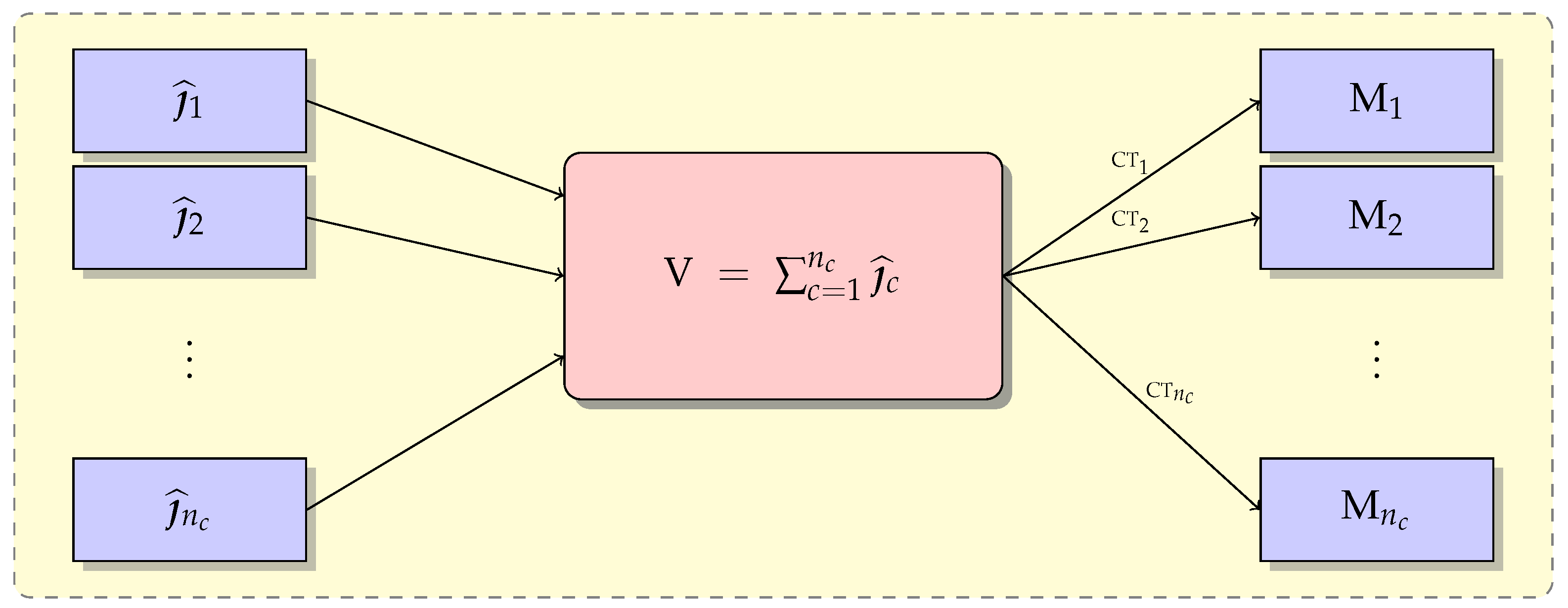
(i)

Add the binary images ${\widehat{\mathit{j}}}_c$ to produce the frequency matrix ($\mathit{V}$).

(ii)

Use automatic optimal thresholds ranging from $t=1,\dots ,n_c$ on $\mathit{V}$ to generate matrices ${\mathit{M}}_t$.

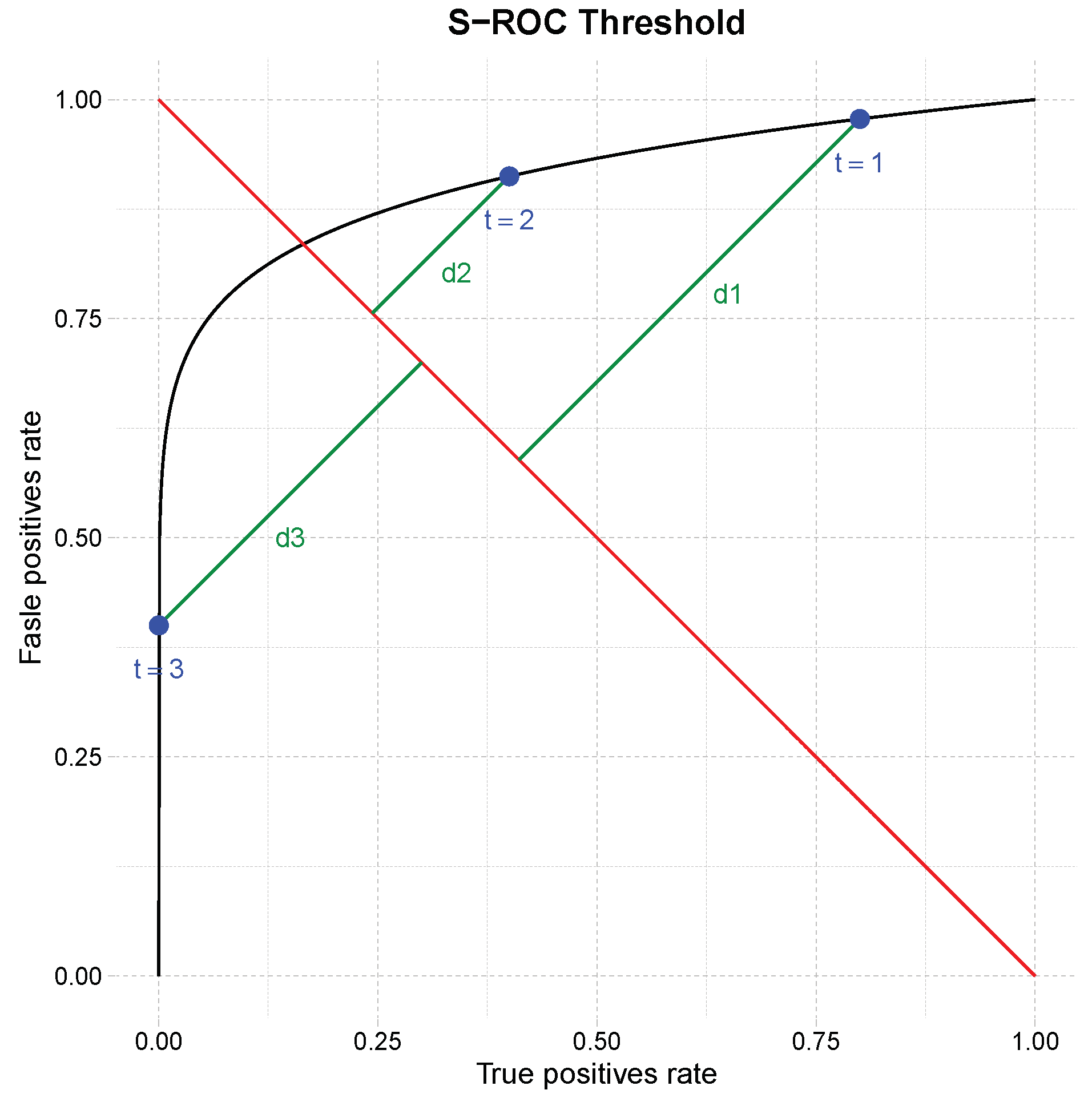
(iii)

Compare each ${\mathit{M}}_t$ with all ${\widehat{\mathit{j}}}_c$, find the confusion matrix, and generate the ROC curve. The optimal threshold corresponds to the point of the ROC curve at the smallest Euclidean distance to the diagnostic line.

(iv)

Use PCA information to choose the channels that will be fused: only those above a threshold ($\tau$) will enter the S-ROC procedure. We used 10% of the sum of the PCA coefficients as the threshold. We named these methods by $\tau$S-ROC.

(v)

The fusion ${\mathit{I}}_F$ is the matrix ${\mathit{M}}_t$ which corresponds to the optimal threshold.

We generate binary images in which one denotes evidence of edge: ${\widehat{\mathit{j}}}_c$, being $c=1,\dots ,n_c$, where $n_c$ is the number of channels. Build the frequency matrix V of the same size as ${\widehat{\mathit{j}}}_c$, such that each position stores the frequency of occurrences of edge evidence in each channel ${\widehat{\mathit{j}}}_c$; i.e., V is the pixel by pixel sum of all edge evidence images ${\widehat{\mathit{j}}}_c$. The larger the pixel value is, the higher its chance of being an edge. Apply thresholds ${\mathrm{CT}}_t$, $t=1,\dots ,n_c$, to V and generate the edge evidence maps ${\mathrm{M}}_t$. The goal of this step is to estimate the optimal global threshold from the set of partial thresholds ${\mathrm{CT}}_t$. Figure 4 shows the flowchart corresponding to this process.

Figure 5 shows the comparison for each ${\mathrm{M}}_t$ matrix, t fixed, with all ${\widehat{\mathit{j}}}_c$ matrices, with $c=1,\dots ,n_c$ resulting in the probabilities true positive ${\mathrm{TP}}_c$, false positive ${\mathrm{FP}}_c$, true negative ${\mathrm{TN}}_c$, and false negative ${\mathrm{FN}}_c$. Furthermore, we define the means true positive ${\overline{\mathrm{TP}}}_c$, false positive ${\overline{\mathrm{FP}}}_c$, true negative ${\overline{\mathrm{TN}}}_c$, and false negative ${\overline{\mathrm{FN}}}_c$ as

$$\begin{array}{cc}\hfill {\overline{\mathrm{TP}}}_t& =\frac{1}{n_c}\sum _{c=1}^{n_c}{\mathrm{TP}}_c^t;\hfill \end{array}$$

(12)

$$\begin{array}{cc}\hfill {\overline{\mathrm{FP}}}_t& =\frac{1}{n_c}\sum _{c=1}^{n_c}{\mathrm{TN}}_c^t;\hfill \end{array}$$

(13)

$$\begin{array}{cc}\hfill {\overline{\mathrm{TN}}}_t& =\frac{1}{n_c}\sum _{c=1}^{n_c}{\mathrm{FP}}_c^t;\hfill \end{array}$$

(14)

$$\begin{array}{cc}\hfill {\overline{\mathrm{FN}}}_t& =\frac{1}{n_c}\sum _{c=1}^{n_c}{\mathrm{FN}}_c^t.\hfill \end{array}$$

(15)

The notation ${\overline{\cap \widehat{\mathit{j}}}}_c$ means that the comparison is performed pixel by pixel as the intersection between ${\mathrm{M}}_t$ and ${\widehat{\mathit{j}}}_c$, averaging according to (12)–(15). The notation + refers to the average of all ${\mathrm{TP}}_c$, or other probabilities ${\mathrm{FP}}_c$, ${\mathrm{FN}}_c$ and ${\mathrm{TN}}_c$.

In the sequence, we find the true positive and false negative ratios for each edge map ${\mathrm{M}}_t$ as:

$$\begin{array}{c}\hfill {\mathrm{TP}}_{rat{e}_t}=\frac{{\overline{\mathrm{TP}}}_t}{{\overline{\mathrm{TP}}}_t+{\overline{\mathrm{FN}}}_t},\end{array}$$

(16)

and

$$\begin{array}{c}\hfill {\mathrm{FP}}_{rat{e}_t}=\frac{{\overline{\mathrm{FP}}}_t}{{\overline{\mathrm{FP}}}_t+{\overline{\mathrm{TN}}}_t}.\end{array}$$

(17)

The values of the false positive ratios, ${\mathrm{FP}}_{rat{e}_t}$, are measured on the horizontal axis, and the true positive ratios, ${\mathrm{TP}}_{rat{e}_t}$, are measured on the vertical axis. Thus, each edge map ${\mathrm{M}}_t$ produces a point on the two-dimensional graph $({\mathrm{FP}}_{rat{e}_t},{\mathrm{TP}}_{rat{e}_t})$.

The optimal CT threshold, corresponding to the parameter t that generates the point $({\mathrm{FP}}_{rat{e}_t},{\mathrm{TP}}_{rat{e}_t})$ at the shortest Euclidean distance to the diagnostic line, determines the image ${\mathrm{M}}_t$ with the highest accuracy of detected edges.

We illustrate this technique in Figure 6. The points $t_1$, $t_2$, and $t_3$ correspond to three images. The diagnostic line is in red, and the distances between the points and this line are the green segments. As $t_2$ is the closest point to the diagnostic line, the optimal threshold is $C{T}_2$, and the image ${\mathrm{M}}_2$ performs best in the edge detection task.

2.7. Measures of Quality

We used the Hausdorff distance (Hd) to measure the performance of the edge estimation by S-ROC and $\tau$S-ROC fusion. This metric is defined as

$$\mathrm{Hd}=\underset{p\in P}{max}\underset{p^{\prime }\in P^{\prime }}{min}\parallel p-p^{\prime }\parallel ,$$

where P and ${\mathrm{P}}^{\prime }$ are points in the actual (ground reference—GR) and estimated edge points. The smaller the Hd value is, the better the edge is. For details, see Refs. [10,29].

3. Results

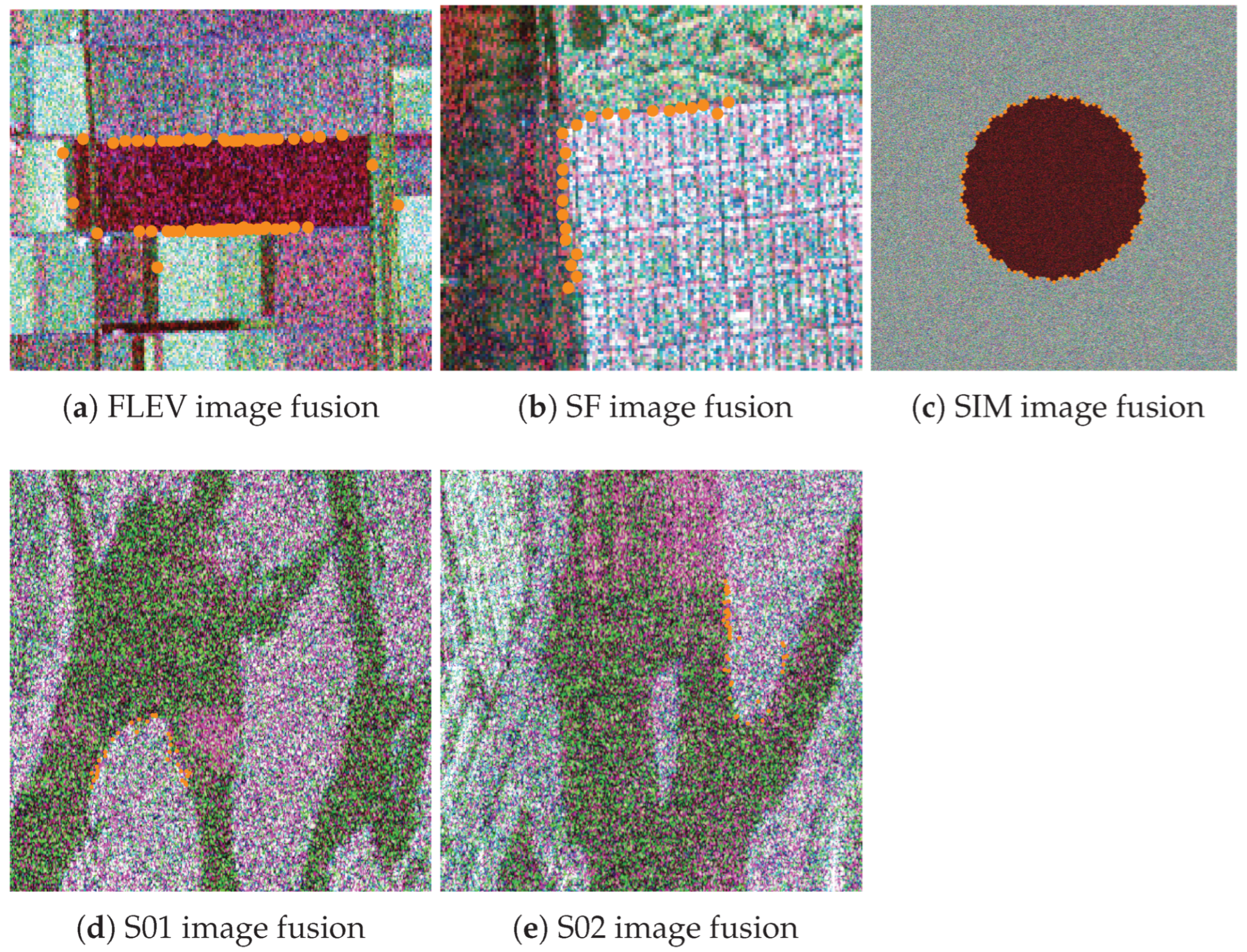
3.1. Flower Simulated Image

For the Flower with dimension $800\times 800$ pixels, we defined the slack constant as 10 pixels, 100 radii, and each radius with 300 pixels. The image has four nominal looks and nine channels.

Figure 7 shows the HH/VV (Figure 7a) and VV/HH (Figure 7b) ratios.

Figure 8 shows the detected points overlain on the Pauli false-color image. We show two good (HH in Figure 8a and span in Figure 8b), and two poor (HH/VV in Figure 8c and VV/HH in Figure 8d) results to emphasize the need to measure the performance and use this information in the fusion process. Figure 9 and Figure 10 show the same analysis but with PolSAR images.

3.2. Flevoland Images

The FLEV image has $750\times 1024$ pixels with four nominal looks. For this image, we defined slacks of 15 pixels, and 100 radii, each with 120 pixels. Zero-valued pixels are removed to avoid division by zero or logarithm applied to zero.

Figure 9 shows examples of good (HH in Figure 9a and span in Figure 9b) and poor (HH/VV in Figure 9c and VV/HH in Figure 9d) detections.

3.3. San Francisco Image

The San Francisco (SF) image has dimension $450\times 600$ pixels, with four nominal looks and nine channels. We defined slacks of 25 pixels and 25 radii with 120 pixels. Again, zero-valued pixels are discarded.

Figure 10 shows examples of good (HH in Figure 10a and span in Figure 10b) and poor (HH/VV in Figure 10c and VV/HH in Figure 10d) detections.

The ratio images provide little edge information. This was observed in all the images from actual sensors. Therefore, Figure 9 and Figure 10 illustrate the need to incorporate some quality measure in the fusion, which we perform with the $\tau$S-ROC fusion.

Figure 11 shows the ratio intensities image. The reason for the poor performance of the detection with ratio images is apparent with the San Francisco image.

3.4. Sub-Scene 01 of Santos City

Figure 12 shows the Pauli false-color composition of a high-resolution image acquired with one look by OrbiSAR-2 over Santos City, Brazil, in P-band. The image has $400\times 400$ pixels and 1 m per pixel. The slack has 15 pixels for this image and 50 radii of 90 pixels each. Zero-valued pixels are removed. Furthermore, the evidence edge detection visualization follows the same construction as before.

Figure 12 shows the results built with univariate gamma and span distributions. Channels HH, VV, and Span lead to accurate detection; see Figure 12a,c,d. Channel HV does not provide good information; see Figure 12b.

Figure 13c,d shows edge estimates obtained with the ratios of intensities; they perform very poorly. Such poor performance can be explained by the lack of visual evidence of edge in the ratio images, as shown in Figure 13a,b.

The methodology applied to image S02 of Santos City presents similar behavior as image S01, and we omit those results for brevity.

3.5. Hd Metric Applied to Edge Evidence Estimates

Table 1. Hausdorff Distance—Hd.

Index	Channel (PDF)	FLEV	SF	S01	S02	SIM
1	Gamma (HH)	31.78	13.60	14.86	11.18	8.24
2	Gamma (HV)	14.00	40.04	33.37	28.00	7.61
3	Gamma (VV)	76.00	22.00	35.84	11.66	8.06
4	Gamma for the span	52.00	29.00	10.63	9.05	7.61
5	PDF ratio (HH/HV)	70.00	25.31	36.24	53.60	10.77
6	PDF ratio (HH/VV)	79.00	38.00	35.84	53.03	115.10
7	PDF ratio (HV/VV)	37.00	29.00	37.01	44.01	12.08
8	PDF ratio (HV/HH)	19.00	25.31	36.24	53.60	10.77
9	PDF ratio (VV/HV)	64.00	26.47	37.01	44.01	12.08
10	PDF ratio (VV/HH)	79.00	38.00	37.64	51.00	115.10

shows the Hd metric applied to the edge estimates from the images defined in items 1 to 4b.

Notably, Table 1 quantifies the poor performance of the method with the ratios of intensities, as verified in the corresponding images for these channels. The span shows good performance, in agreement with the results shown.

3.6. PCA Analysis

The columns of

Table 2. PCA Coefficients.

Channel (PDF)	FLEV	SF	S01	S02	SIM
Gamma (HH)	29.04	28.34	24.00	22.71	53.28
Gamma (HV)	18.86	19.95	18.78	18.21	19.90
Gamma (VV)	17.43	18.20	15.52	15.77	12.09
Gamma for the span	0.19	13.47	13.91	14.69	9.06
PDF ratio (HH/HV)	2.36	7.75	9.09	10.02	0.36
PDF ratio (HH/VV)	8.92	5.21	8.77	8.65	0.18
PDF ratio (HV/VV)	4.55	2.66	4.54	5.07	0.00
PDF ratio (HV/HH)	5.46	2.08	4.95	4.19	0.00
PDF ratio (VV/HV)	5.60	1.46	4.00	0.44	0.00
PDF ratio (VV/HH)	7.53	0.40	0.00	0.22	0.00

show the weight with which each detection channel enters the principal component decomposition. Notice that, in all cases, the individual intensities are the most relevant channels. The span follows them in all cases except in the Flevoland data set.

We use the PCA analysis to quantify the influence of each channel and then choose the most relevant for the fusion process. We chose the threshold empirically to 10%, with good results.

3.7. S-ROC and $\tau$S-ROC Information Fusion

Table 3. Hd applied to the results of information fusion techniques.

Fusion	S-ROC	$\mathit{\tau }$S-ROC	$\mathit{\tau }$S-ROC
	(All Channels)	(Selected Channel)	Channels
FLEV	32.00	23.70	HH–HV–VV
SF	12.00	5.09	HH–HV–VV–Span
S01	35.84	10.63	HH–HV–VV–Span
S02	14.21	18.35	HH–HV–VV–Span–HH/HV
SIM	13.03	20.09	HH–HV–VV

shows the Hausdorff distance of the results using (i) all the channels, named here S-ROC, and (ii) the $\tau$S-ROC proposal that selects the channels using principal components.

The images in Figure 14 show the results using $\tau$S-ROC, which are better than those produced by S-ROC (we omit them for brevity). Table 3 presents a quantitative analysis of the Hausdorff distance applied to the results provided by S-ROC and $\tau$S-ROC.

We used the SIM image to quantify the sensitivity of the $\tau$S-ROC method to the variation of $\tau$ because we know the actual edge position.

Table 4. Hd applied to the results of the fusion techniques to examine the sensitivity to $\tau$ variation.

Fusion Methods
S-ROC	$\mathit{\tau }$S-ROC	$\mathit{\tau }$S-ROC
(All Channels)	(Selected Channel)	Channels
	7.61 ($\tau =5\%$)	HH–HV–VV–Span
13.03	20.09 ($\tau =10\%$)	HH–HV–VV
	8.24 ($\tau =20\%$)	HH

was constructed using the S-ROC and $\tau$S-ROC fusion methods applied to the SIM image, varying the threshold values: $\tau =5\%$, $\tau =10\%$, and $\tau =20\%$. The table presents which channels were selected with each threshold.

Table 5. Execution times S-ROC and $\tau$S-ROC consume for detecting edges.

	Mean Time [s]
	Edges Evidence	S-ROC	$\mathit{\tau }$S-ROC
Image	(All Channels)	(All Channels)	(Selected Channels)
FLEV	3136	54	5
SF	656	19	3
S01	645	11	2
S02	975	12	3
SIM	15375	45	4

shows the mean execution times of the methods: edge detection, S-ROC, and $\tau$S-ROC. We applied the methods ten times. The median values were almost the same as the sample means.

3.8. Change Detection

This section uses our edge detection for a new change detection approach.

One of the challenges of finding changes in a noisy field is identifying relevant changes over random fluctuations. To achieve this aim, we calculate the log-likelihood function at each radial point, find the sample mean ($\widehat{\mu }$) and the sample standard deviation $\widehat{\sigma }$, and define a threshold $\xi =\widehat{\mu }\pm \alpha \widehat{\sigma }$. The constant $\alpha =0.25$ was chosen empirically. Only values outside this interval are considered relevant changes.

Figure 2 shows two coregistered images for the same regions in Los Angeles, CA, USA. The Jet Propulsion Laboratory/National Aeronautics and Space Administration (JPL) acquired the images using the Uninhabited Aerial Vehicle Synthetic Aperture Radar (UAVSAR) with L-band polarimetric multilook. Figure 2a was acquired on 23 April 2009, and Figure 2b on 11 May 2015. The images have $760\times 300$ pixels.

We apply the two methodologies, namely, the standard one and after applying the threshold to the LAA image; Figure 15 shows the results. Figure 15a shows the standard methodology, which shows the presence of outliers. Figure 15b shows the results thresholding by the likelihood; it performs well and does not wrongly identify edges on the relatively flat area. The edge estimates agree with the transition between the two regions. We only show channel HH; however, the results are consistent along all channels: thresholding by the likelihood systematically reduces the number of false positives and, at the same time, does not noticeably increase the number of false negatives.

The images in Figure 16 show Pauli decompositions in gray-scale overlaid with edge evidence (Figure 16a,b) and edge detected with S-ROC and $\tau$S-ROC (Figure 16c,d). The results shown in this figure were built thresholding by the likelihood of the points in each ray.

The images in Figure 17 show Pauli decomposition in gray-scale overlaid with edge evidence (Figure 17a,b) and edges detected with information fusion (Figure 17c,d). The results shown in this figure were built thresholding by the likelihood.

Change detection in multilook polarimetric image SAR (PolSAR) with the methods to detect the edge evidence and thresholding works accurately. The images in Figure 18a,b show the result of applying $\tau$S-ROC.

4. Discussion

The main results we obtained are summarized in the following:

(i)

Although the estimation by maximization of the log-likelihood with the BFGS algorithm is stable, it is most sensitive to the initial point with the distribution of ratios. We used the first- and second-order moments estimates with good results.

(ii)

Table 2 shows that the PCA method recommends the fusion of the intensities or span channels, except in image S02; we used these channels to build the fusion methods $\tau$S-ROC.

(iii)

The $\tau$S-ROC method performs best concerning Hd.

(iv)

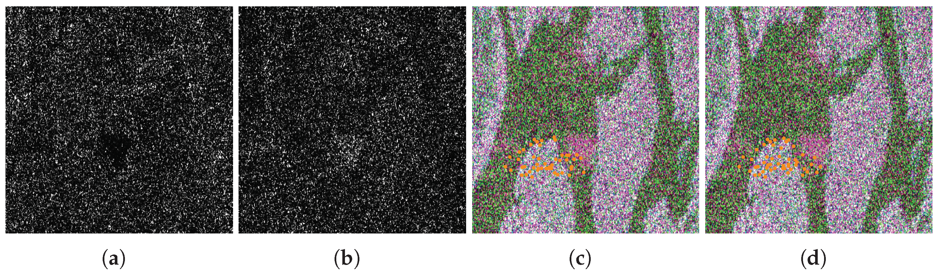
S02 (Figure 1) is a unique data set in which the ratio of intensities contributes to the $\tau$S-ROC fusion.

(v)

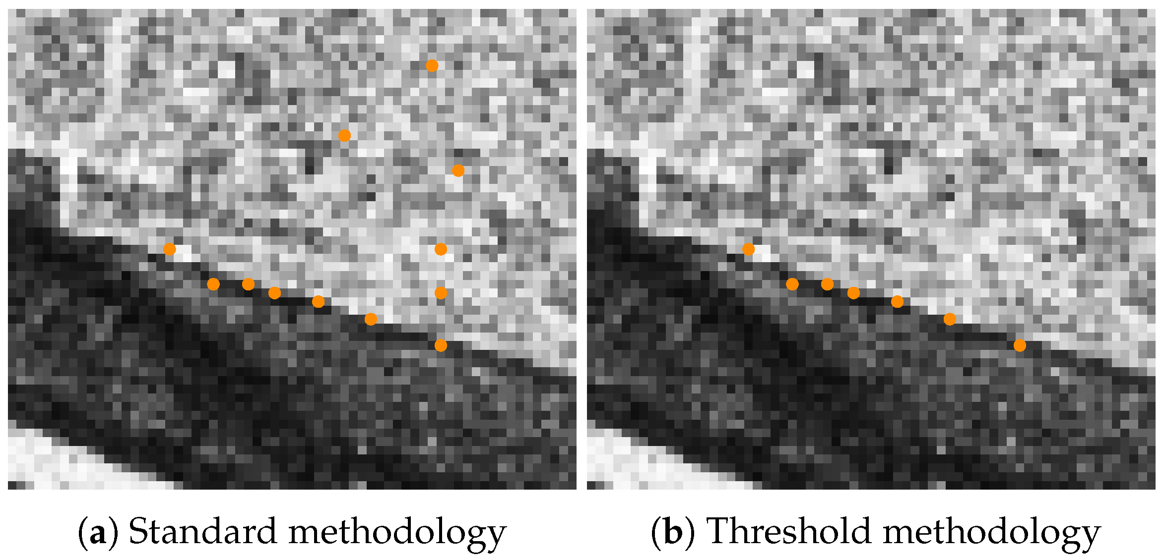
$\tau$S-ROC is better than S-ROC at discarding outliers.

(vi)

S-ROC and $\tau$S-ROC work well in images from various sensors.

(vii)

$\tau$S-ROC rejects false positive detection on homogeneous areas.

(viii)

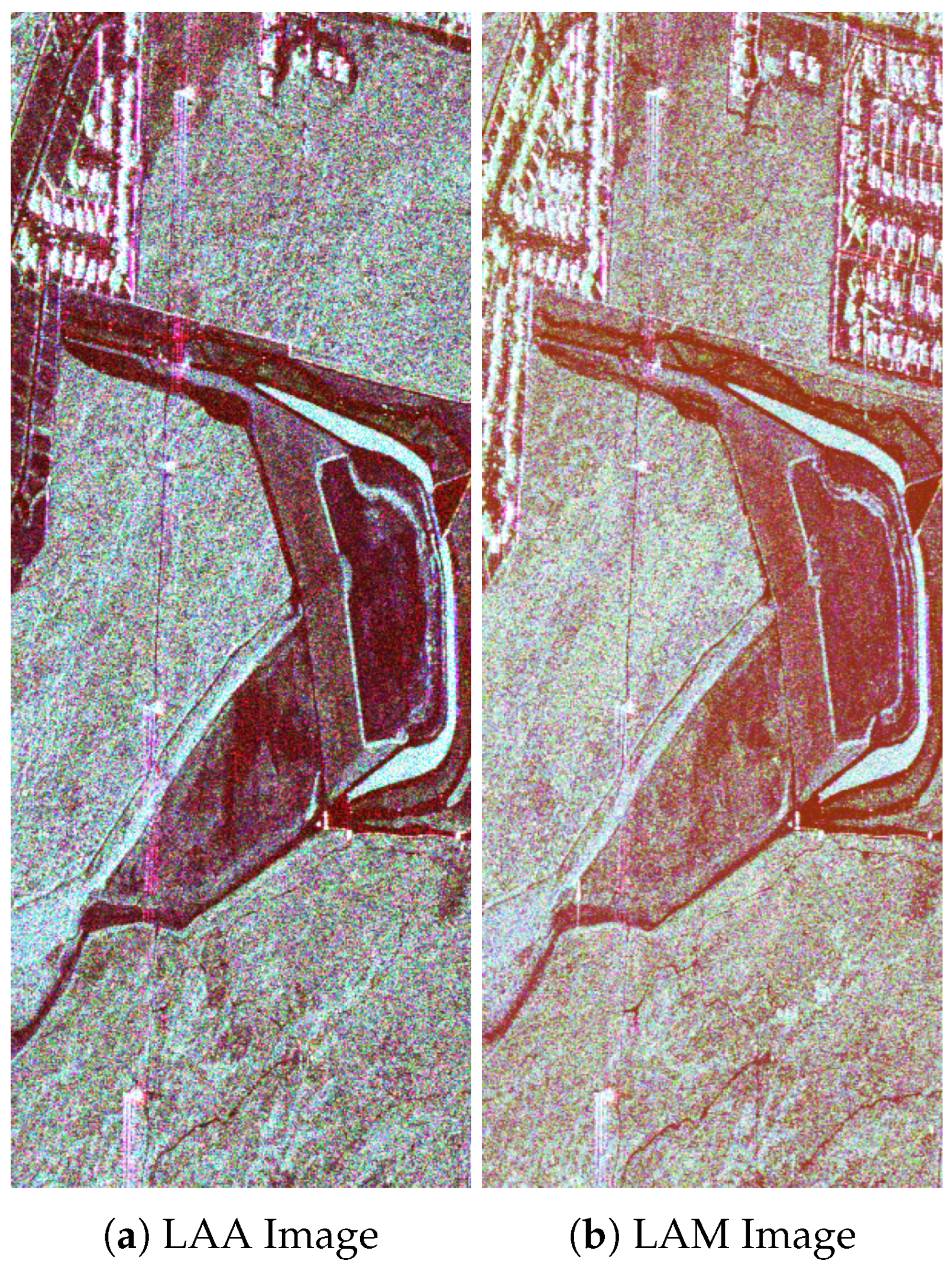
Figure 16 and Figure 17 show the thresholding results by the likelihood using the HH, and Span channels, and edge detection by S-ROC and $\tau$S-ROC. These results motivated us to check the change detection in two images of Los Angeles taken from the same region at different times. The result is shown in Figure 18. The visual inspection of Figure 18a (LAA image) and Figure 18b (LAM image) shows the method’s ability to identify changes.

(ix)

We used images with different numbers of looks: images S01 and S02 are single-look, while the others have four; our methods present similar performance.

5. Conclusions

Using the ratio channels does not improve edge detection. Even when some ratio channels contribute to edge detection, as in the case of image S02, see Table 3, the value of the PCA coefficient is very close to the threshold; cf. Table 2.

The span produces the best Hd; this result is compatible with the high visual quality of the span images. Including span in the fusion process is, thus, a recommendation. The worst detection performance occurs when using the HH/VV and VV/HH channels; therefore, including these bands in the process is not recommended.

The $\tau$S-ROC is a suitable approach for edge and change detection. It is computationally more efficient than S-ROC, cf. Table 5. The thresholding operation is fast, and using fewer channels compensates for this step.

Extracting the edge evidence is the most time-consuming state of the processing pipeline. Under the Gambini algorithm, the detection of each ray can be implemented as an independent thread. This approach is, thus, suitable for distributed and parallel architectures.

Thresholding by the likelihood rejects false positives and, thus, is adequate for change detection.

The information captured by the $\tau$S-ROC method can be improved by adding optical channels and ancillary information in the fusion process in the form of other physically-based and/or empirical models.

References

- Blake, A.; Isard, M. Active Contours; Springer: Berlin/Heidelberg, Germany, 1998. [Google Scholar]
- Szeliski, R. Computer Vision: Algorithms and Applications, 2nd ed.; Springer: Berlin/Heidelberg, Germany, 2022. [Google Scholar]
- Gambini, J.; Mejail, M.; Jacobo-Berlles, J.; Frery, A.C. Feature Extraction in Speckled Imagery using Dynamic B-Spline Deformable Contours under the G0 Model. Int. J. Remote Sens. 2006, 27, 5037–5059. [Google Scholar] [CrossRef]
- Gambini, J.; Mejail, M.; Jacobo-Berlles, J.; Frery, A.C. Accuracy of Edge Detection Methods with Local Information in Speckled Imagery. Stat. Comput. 2008, 18, 15–26. [Google Scholar] [CrossRef]
- Frery, A.C.; Jacobo-Berlles, J.; Gambini, J.; Mejail, M. Polarimetric SAR Image Segmentation with B-Splines and a New Statistical Model. Multidimens. Syst. Signal Process. 2010, 21, 319–342. [Google Scholar] [CrossRef]
- Nascimento, A.D.C.; Horta, M.M.; Frery, A.C.; Cintra, R.J. Comparing Edge Detection Methods Based on Stochastic Entropies and Distances for PolSAR Imagery. IEEE J. Sel. Top. Appl. Earth Obs. Remote Sens. 2014, 7, 648–663. [Google Scholar] [CrossRef]
- Naranjo-Torres, J.; Gambini, J.; Frery, A.C. The Geodesic Distance between GI0 Models and its Application to Region Discrimination. IEEE J. Sel. Top. Appl. Earth Obs. Remote Sens. 2017, 10, 987–997. [Google Scholar] [CrossRef]
- Girón, E.; Frery, A.C.; Cribari-Neto, F. Nonparametric edge detection in speckled imagery. Math. Comput. Simul. 2012, 82, 2182–2198. [Google Scholar] [CrossRef]
- Borba, A.A.D.; Marengoni, M.; Frery, A.C. Fusion of Evidences in Intensities Channels for Edge Detection in PolSAR Images. IEEE Geosci. Remote Sens. Lett. 2022, 19, 1–5. [Google Scholar] [CrossRef]
- Rey, A.; Revollo Sarmiento, N.; Frery, A.C.; Delrieux, C. Automatic Delineation of Water Bodies in SAR Images with a Novel Stochastic Distance Approach. Remote Sens. 2022, 14, 5716. [Google Scholar] [CrossRef]
- Asokan, A.; Anitha, J. Change detection techniques for remote sensing applications: A survey. Earth Sci. Informatics 2019, 12, 143–160. [Google Scholar] [CrossRef]
- Bouhlel, N.; Akbari, V.; Méric, S. Change Detection in Multilook Polarimetric SAR Imagery with Determinant Ratio Test Statistic. IEEE Trans. Geosci. Remote Sens. 2022, 60, 1–15. [Google Scholar] [CrossRef]
- Touzi, R.; Lopes, A.; Bousquet, P. A statistical and geometrical edge detector for SAR images. IEEE Trans. Geosci. Remote Sens. 1988, 26, 764–773. [Google Scholar] [CrossRef]
- Schou, J.; Skriver, H.; Nielsen, A.; Conradsen, K. CFAR edge detector for polarimetric SAR images. IEEE Trans. Geosci. Remote Sens. 2003, 41, 20–32. [Google Scholar] [CrossRef]
- Chapman, B.; Shi., J. CLPX-Airborne: Airborne Synthetic Aperture Radar (AIRSAR) Imagery, Version 1 [Data Set]; NASA National Snow and Ice Data Center Distributed Active Archive Center: Boulder, CO, USA, 2004. [Google Scholar] [CrossRef]
- Bouhlel, N.; Akbari, V.; Méric, S. Change Detection in Multilook Polarimetric SAR Imagery with DRT Statistic. IEEE Dataport 2021. [Google Scholar] [CrossRef]
- Nobre, R.; Rodrigues, A.; Rosa, R.; Medeiros, F.; Feitosa, R.; Estevão, A.; Barros, A. GRSS SAR/PolSAR Database. IEEE Dataport 2017. [Google Scholar] [CrossRef]
- Long, D.G.; Ulaby, F.T. Microwave Radar and Radiometric Remote Sensing; The University of Michigan Press: Norwood, MI, USA, 2014. [Google Scholar]
- Goodman, N.R. Statistical Analysis Based on a Certain Complex Gaussian Distribution (an Introduction). Ann. Math. Stat. 1963, 34, 152–177. [Google Scholar] [CrossRef]
- Lee, J.S.; Hoppel, K.W.; Mango, S.A.; Miller, A.R. Intensity and phase statistics of multilook polarimetric and interferometric SAR imagery. IEEE Trans. Geosci. Remote Sens. 1994, 32, 1017–1028. [Google Scholar] [CrossRef]
- Hagedorn, M.; Smith, P.J.; Bones, P.J.; Millane, R.P.; Pairman, D. A trivariate chi-squared distribution derived from the complex Wishart distribution. J. Multivar. Anal. 2006, 97, 655–674. [Google Scholar] [CrossRef]
- Ferreira, J.A.; Nascimento, A.D.C.; Frery, A.C. PolSAR Models with Multimodal Intensities. Remote Sens. 2022, 14, 5083. [Google Scholar] [CrossRef]
- Feng, Y.; Wen, M.; Zhang, J.; Ji, F.; Ning, G. Sum of arbitrarily correlated Gamma random variables with unequal parameters and its application in wireless communications. In Proceedings of the 2016 International Conference on Computing, Networking and Communications (ICNC), Kauai, HI, USA, 15–18 February 2016; pp. 1–5. [Google Scholar]
- Henningsen, A.; Toomet, O. maxLik: A package for maximum likelihood estimation in R. Comput. Stat. 2011, 26, 443–458. [Google Scholar] [CrossRef]
- Xiang, Y.; Gubian, S.; Suomela, B.; Hoeng, J. Generalized Simulated Annealing for Global Optimization: The GenSA Package. R J. 2013, 5, 13–28. [Google Scholar] [CrossRef]
- Giannarou, S.; Stathaki, T. Optimal edge detection using multiple operators for image understanding. EURASIP J. Adv. Signal Process. 2011, 2011, 28. [Google Scholar] [CrossRef]
- Naidu, V.P.S.; Raol, J.R. Pixel-level Image Fusion using Wavelets and Principal Component Analysis. Def. Sci. J. 2008, 58, 338–352. [Google Scholar] [CrossRef]
- Mitchell, H. Image Fusion: Theories, Techniques and Applications; Springer: Berlin/Heidelberg, Germany, 2010. [Google Scholar]
- Taha, A.A.; Hanbury, A. An Efficient Algorithm for Calculating the Exact Hausdorff Distance. IEEE Trans. Pattern Anal. Mach. Intell. 2015, 37, 2153–2163. [Google Scholar] [CrossRef] [PubMed]