Abstract
Deception jamming of synthetic aperture radar (SAR) has attracted extensive attention due to its low power consumption and high fidelity advantages. However, existing SAR deception jamming algorithms assume that SAR operates on a linear trajectory. In practice, SAR trajectories often become nonlinear due to factors such as atmospheric turbulence, which results in the jamming signals lacking the two-dimensional spatial variability of nonlinear-trajectory SAR echo signal and affects the imaging quality of deception jamming. This paper proposes a new algorithm for nonlinear-trajectory airborne SAR deception jamming based on hybrid domain efficient (HDE) modulation. This algorithm derives the jamming frequency response (JFR) with SAR trajectory deviation in the azimuth time–frequency hybrid domain. Based on the hybrid domain modulation, the jammer calculates the JFR of the linear trajectory in the azimuth frequency domain and constructs for the real-time trajectory deviation pulse by pulse at each azimuth moment. The real-time modulation process of the algorithm only involves range domain Fourier transform and complex multiplication, combining computational efficiency and modulation flexibility. The validity constraints of the algorithm have been analyzed to ensure the focusing ability of the jamming signal. Simulation and computational complexity analysis validate the excellent performance of the algorithm in imaging quality and efficiency.
1. Introduction
Synthetic Aperture Radar (SAR) is an active microwave imaging system that uses electromagnetic waves for two-dimensional high-resolution imaging, which has many advantages, such as all-day, all-weather, strong penetration capability, high processing gain, and strong anti-jamming capability [1]. It is widely used in strategic reconnaissance, strike effect assessment, and other military occasions and has become a significant method to obtain information in modern warfare. Its powerful and flexible functions can substantially threaten high-value strategic targets, military facilities, and intelligence security. Therefore, to protect sensitive targets and sensitive areas, electronic countermeasures against SAR have received extensive attention and development [2,3,4,5].
According to the different jamming effects, active jamming techniques for SAR are divided into barrage jamming and deceptive jamming. Barrage jamming uses high-powered noise to attenuate the signal to jamming ratio within a specific region to cover up the real target [6,7,8,9].The deceptive jamming confuses target identification without causing enemy awareness by directly generating or modulating-retransmitting false target echo signals and implanting false electromagnetic features in SAR radar images [10,11,12,13,14,15,16,17,18,19,20,21,22,23,24]. Compared with barrage jamming, deceptive jamming is characterized by higher concealment, lower power consumption and more flexible application scenarios. Therefore, deceptive jamming is more attractive and promising.
The modulation and retransmission mechanism is currently the mainstream research approach for SAR deception jamming [25,26]. The deceptive jammer based on the modulation-retransmission mechanism can be modeled as a linear time-invariant system. In each pulse repetition interval (PRI), the jamming system generates a frequency response function based on a series of parameters such as platform parameters, antenna parameters, and signal parameters of the SAR to be jammed [10,11]. The basic scheme of modulation-retransmission deceptive jamming is to modulate and retransmit the spectrum of intercepted pulses with the frequency response function of the jamming system to produce a jamming signal, which is imaged by the SAR receiver to form a false target. The traditional algorithm is the point-by-point superposition straightforward calculation algorithm (SA), which directly calculates the difference in signal propagation delay between each scatter point in the deceptive jammer template and the jammer during each PRI. However, this algorithm involves the iterative operation by the double integral in continuous pulses, and it is challenging to guarantee real-time modulation calculation [11]. Several algorithms have been proposed to reduce the computational burden to fulfill real-time jamming and have been divided into two categories: azimuth time-domain processing and azimuth frequency-domain processing. The former reduces computational complexity through slant-range approximation equations and range-azimuth split-dimensional modulation, which can cause a loss of image quality to a certain extent, including the segmented modulation algorithms [14,15], the multi-receiver approximation algorithms [16,17] and the time-delay frequency-shifting algorithms with template segmentation [22]. The latter requires azimuth Fourier transform modulation processing on the template, which is relatively precise but faces obstacles in practicality due to some defects, such as the low-efficiency interpolation calculation [27,28], including the inverse range-Doppler algorithm [12], the frequency domain three-stage algorithm [19], the inverse Omega-K algorithm [20], and the frequency domain pre-modulation algorithm [18].
All the above algorithms assume SAR has a nominal linear trajectory and perform partial calculations of slant range before real-time modulation. However, in practical situations, SAR platforms may deviate from the nominal linear trajectory due to factors such as changes in airflow. The echo signal received by nonlinear-trajectory SAR will be imaged with motion error compensation [29]. When jamming nonlinear-trajectory SAR, these algorithms cannot construct the azimuth time-varying trajectory deviation phase of the jamming signal pulse by pulse, which will lead to defocusing and shifting of deceptive jamming imaging [30,31,32]. Currently, the deceptive jamming for nonlinear-trajectory SAR can only use the inefficient point-by-point superposition direct calculation algorithm (SA) [11], To sum up, for nonlinear-trajectory SAR with trajectory deviation in actual combat, how to consider the calculation efficiency and the ability to construct trajectory deviation pulse by pulse is a challenge for SAR deceptive jamming in practical applications. This paper proposes a nonlinear-trajectory SAR deceptive jamming algorithm based on a hybrid domain efficient modulation (HDE). The HDE algorithm simulates the SAR jammer’s frequency response function with trajectory deviation in the time–frequency hybrid domain. It decomposes the coupling term of the trajectory deviation and JFR function with the assumption of center beam approximation and trajectory deviation constraints. The frequency response function of the deceptive jamming template is computed in the azimuth frequency domain, and the real-time trajectory deviation term is constructed in the azimuth time domain. The HDE algorithm combines the efficiency of azimuth frequency-domain processing with the flexibility of azimuth time-domain processing, allowing for efficient and accurate generation of deceptive signals for nonlinear-trajectory SAR. It solves the problem of real-time deceptive jamming against nonlinear-trajectory SAR and has the potential for practical application in SAR jamming.
The paper is organized as follows. Section 2 provides a detailed derivation of the HDE algorithm. Section 3 gives the workflow and validity constraints of the HDE algorithm implementation. Section 4 describes the simulation with experimental validation of the HDE algorithm and analyzes the algorithm’s computational complexity. Section 5 discusses the HDE algorithm through effectiveness analysis and experimental results. Section 6 concludes this paper.
2. Nonlinear-Trajectory SAR Deception Jamming Algorithm Based on HDE
This section will systematically derive the HDE-based nonlinear-trajectory deceptive jamming algorithm. First, the geometric model of the nonlinear-trajectory SAR system is introduced, then the principle of SAR deceptive jamming is presented, and finally, the principle of the HDE algorithm is derived in detail.
2.1. Nonlinear-Trajectory SAR System Model
Taking side-looking Stripmap SAR as an example, when the jammer interferes with the nonlinear-trajectory SAR system, the geometric relationship between the SAR, the jammer, and the deceptive area is shown in Figure 1. Where the origin O of the spatial coordinate system is located at the flight start point of the SAR radar, is the trajectory of the radar. The X-axis points to the azimuth direction, the Y-axis points to the range direction, and the Z-axis points to the height direction. Vector represents the absolute deviation vector of the nonlinear-trajectory relative to the nominal trajectory. The y and z components of vector represent the horizontal and vertical deviation of the SAR flight platform relative to the nominal trajectory. represents the angle of the flight trajectory deviation relative to the nominal trajectory, and is the SAR antenna elevation angle. The jammer is placed at point , represents an arbitrary point in the deceptive region P, and the point on the center of the beam with the same nearest slant range and height as it is . and are the local look angles of points P and J. is the shortest slant range between the radar antenna and point P in the nominal trajectory, and are the slant range from the target P to the antenna in the generic antenna position for nonlinear and nominal trajectories, is the ground range offset of point P with respect to the scene centroid, respectively.
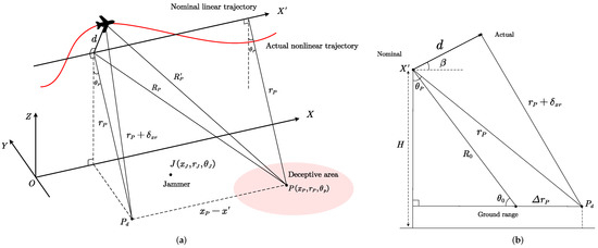
Figure 1.
Nonlinear trajectory SAR spatial geometry model. (a) Three-dimension view; (b) Two-dimension cross trajectory view.
Assume that the SAR transmitted signal is a chirp pulse, as follows:
where t is the fast time, f is the carrier frequency, and and are the chirp pulse duration and rate, respectively. The spatial domain expression of the nonlinear-trajectory SAR echo signal in the deceptive aera P is [33]:
where is the actual position of SAR radar, is the range spatial sampling interval and c is the speed of light. is the antenna ground illumination pattern, is the synthetic aperture length, and L is the azimuth length of the physical antenna. is the target reflectivity. is the carrier wavelength, is the signal bandwidth. From the geometry shown in Figure 1, the slant ranges and take the forms:
The geometry from cross trajectory view is shown in Figure 1, so the term is given by:
where are related to the horizontal and vertical trajectory deviation of the SAR radar. The slant range can be separated as follows [29,33]:
where is the space-invariant trajectory deviation of the scene center, represents the projection of the trajectory deviation on the scene center, and depends only on the SAR radar azimuth coordinate . is the range space-variant trajectory deviation, represents the range space-variant behavior of the line-of-sight direction trajectory deviation, and depends on the SAR radar azimuth coordinate and the local look angles of points :
is the azimuth space-variant trajectory deviation, which depends on the SAR radar azimuth coordinate , the range and azimuth coordinate of point :
The three trajectory deviation terms above can be calculated by Equation (5).
2.2. Nonlinear-Trajectory SAR Deception Jamming Principle
First, we illustrate the geometric relationship between jammer, deceptive area, and SAR by establishing a coordinate system: SAR radar coordinates and jammer coordinates in the two-dimensional slant-range plane, as shown in Figure 2. The dashed line on the axis corresponds to the nominal linear trajectory of the SAR radar, and the curve on the axis is the actual nonlinear-trajectory of the SAR radar. The spatial origin is at jammer. Then the jammer is located at in the coordinate system, represents the shortest slant range between the jammer and the radar. Denote location of an arbitrary false target by in deceptive area, and its scattering coefficient is , and represent the instantaneous slant range of false target P and jammer J at the SAR radar azimuth position , respectively.
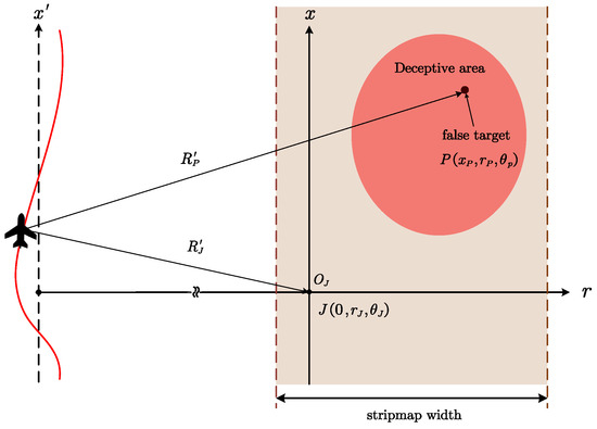
Figure 2.
Two-dimension slant range plane geometric model for SAR deceptive jamming.
An implementation scheme of SAR deceptive jamming based on modulation-retransmission is presented in Figure 3. The jammer needs amplification, down-conversion, analog to digital (A/D) conversion, and Fourier transform of the intercepted SAR radar signal to obtain the baseband range frequency domain signal, multiply it with the jamming frequency response (JFR) and then perform inverse Fourier transform, digital to analog (D/A) conversion, up-conversion and gain control to generate the jamming signal and forward it to the SAR radar. Therefore, the JFR is the key to deceptive jamming modulation. Equation (2) is expressed in the range frequency domain form by the stationary phase method:
where . represents range frequency. The double integral term is the transfer function of the SAR system. Equation (9) combined with Figure 2, the JFR can be obtained as:
where is the instantaneous slant range between and :
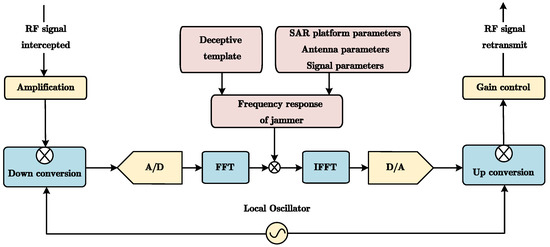
Figure 3.
Principle of SAR deceptive jamming based on modulation-retransmission.
Equation (10) is the JFR of the traditional point-by-point superposition direct calculation algorithm (SA) [11]. The jammer calculates different JFRs in each pulse according to Equation (10), which can achieve jamming modulation of the deceptive template. Due to the dependence of nonlinear-trajectory deceptive jamming on real-time trajectory deviation, the jammer needs to update the JFR for each PRI. However, the SA algorithm involves double integration calculations under continuous pulses, which results in a large computation load and makes it difficult to ensure the flexible and efficient calculation of JFR. Therefore, it is necessary to calculate the JFR more efficiently and flexibly.
2.3. Deceptive Jamming Based on HDE
In this section, the HDE deceptive jamming algorithm will be derived step by step. First, the SAR system-related filter is separated from the SAR JFR. Then, the mathematical derivation of the SAR system-related filter is described in the time–frequency hybrid domain. Finally, the mathematical expression of the HDE deceptive jamming algorithm is clarified.
2.3.1. Decomposition of JFR
Considering the complex double integration operation in JFR, Equation (10) can be decomposed as follows:
where is the jammer-related filter:
In addition, is the SAR system-related filter:
Comparing Equations (13) and (14), we can find that the main computation of SAR JFR comes from Equation (14) and is independent of the relevant parameters of the jammer. To design an efficient algorithm for calculating the JFR, the derivation of Equation (14) with a double integration calculation needs to be performed next.
2.3.2. Fast Algorithm of the SAR System-Related Filter Based on HDE
For nonlinear-trajectory deceptive jamming, it is necessary to avoid calculating trajectory deviation before real-time modulation while ensuring the calculation efficiency of JFR. As far as possible, it is guaranteed that the jammer can construct pulse-by-pulse time-domain trajectory deviations to adapt to the azimuth time-varying trajectory deviations. SAR system-related filters can be represented as:
The space-invariant trajectory deviation term , which does not depend on the target’s position , can be separated from double integration. Thus, the space-invariant trajectory deviation construction of the SAR system-related filter of the jammer can be accomplished in the range frequency domain with only one multiplicative calculation.
We next discuss the feasibility of efficient calculation of in the azimuth frequency domain. The Fourier transform expression of along the azimuth direction is as follows:
where is the azimuth frequency, , is the azimuth frequency. Transform the time-domain term multiplication in the azimuth Fourier transform into a frequency domain term convolution, rearrange its integral expression [33]:
where represents the frequency response function of the nominal linear trajectory SAR, and represents the ground reflectivity term corrected by the space-variant trajectory deviation:
Here,
To facilitate the real-time trajectory deviation construction of the jammer, Equation (17) is transformed into the azimuth time domain for the derivation of the trajectory deviation:
The center beam approximation is assumed in Equation (20), which takes that the motion error associated with all the targets’ positions in the interior of the azimuth beam is equal to the motion error at the center of the azimuth beam. In addition, considering that the range frequency window function in has a limit , there is . Then (20) can be expressed as:
According to the definition of SAR motion compensation [29], the effect of the assumption on imaging can be ignored when the maximum phase error caused by this assumption is much less than 1 rad. The following conditions are met:
Then Equation (22) can be simplified to the following form [34]:
Here, both and represent azimuth Fourier transform:
The meaning of the last integral terms in Equation (25) is to represent the inverse Fourier transform of the convolution of the deviation phase component of the range space-variant trajectory and SAR system frequency response function . Due to the dependence of the function on the item, for a JFR with N points sampled in the range domain, the convolution operation needs to be calculated N times. Such modulation has a high computational time complexity.
However, can be decomposed into the -dependent part and the remaining part [34]:
Here,
When the spectral expansion along the axis is much more minor than the minimum period of oscillation of the , the approximates that it does not vary along the axis within the bandwidth of the . So that can be separated from the convolution calculation along the (this assumption will be analyzed in the next section). It means the convolution operation in the azimuth frequency domain only needs to be calculated once:
Since , we can try to neglect the range-azimuth coupling phase in , and its effect on the jamming signal will be analyzed in Section 3.2. Then can be simplified to the following form:
Here,
The last integral term of Equation (31) represents the inverse Fourier transform of the convolution of the two azimuthal frequency domain terms and , which can be converted into the product of the azimuthal time-domain terms:
Rearrange the integral equation as follows, where represents the range Fourier transform and represents the azimuth inverse Fourier transform:
Combined with Equation (15), the SAR system-related filter is as follows:
Equation (35) realizes the double integral calculation of the deceptive template efficiently in the azimuth frequency domain through azimuth Fourier transform and complex multiplication, and moves the trajectory deviation term to the azimuth time domain. Combined with real-time amplitude modulation and complex multiplication of jammer-related filters Equation (13), the JFR can achieve trajectory deviation construction for deceptive jamming on a pulse-by-pulse basis as follows:
Therefore, the jammer can efficiently and flexibly implement deceptive jamming in the azimuth time–frequency hybrid domain, which is the HDE deceptive jamming algorithm.
3. Workflow and Validity Analysis of HDE Algorithm
In this section, the workflow and validity constraints for the implementation of the HDE deceptive jamming algorithm are described and analyzed.
3.1. HDE Algorithm Workflow
In the workflow of the jammer, obtaining the relevant parameters of the jamming object is the premise of jamming, which mainly includes the following aspects:
- SAR platform parameters, such as SAR flight altitude H, motion velocity v;
- Antenna parameters, such as antenna elevation angle , synthetic aperture length L;
- Signal parameters, such as the carrier frequency f, bandwidth , chirp pulse duration and PRI ;
The above parameters need to be obtained before jamming modulation to estimate the SAR nominal linear trajectory and construct the jamming frequency response function of the SAR nominal linear trajectory. When the jamming object is a nonlinear-trajectory airborne SAR, the trajectory deviation of the SAR also needs to be obtained in real time for the trajectory deviation construction of the HDE algorithm. The specific acquisition methods of these parameters will not be discussed in this paper, and we assume that the parameters have been obtained in advance.
The main workflow of the deceptive jamming algorithm for nonlinear-trajectory SAR based on HDE, as per Equation (36), is illustrated in Figure 4. The workflow of the HDE algorithm encompasses two stages: jammer initialization and real-time computation.
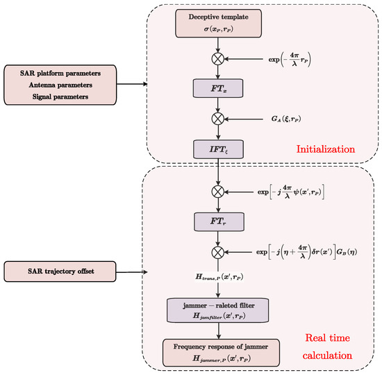
Figure 4.
Hybrid domain efficient (HDE) deceptive jamming algorithm workflow.
- (1)
- The first stage is jammer initialization. First, a deceptive template with complex backscatter coefficients is obtained. Then according to the SAR platform parameters and signal parameters, the jammer performs the phase compensation of the shortest slant range on the deceptive template and combines the antenna parameters to construct the azimuth frequency modulation term of the deceptive template in the SAR azimuth frequency domain. Finally, the azimuth frequency modulation term is converted to the azimuth time domain to form an initialization template for the jammer to perform trajectory deviation construction in the real-time calculation stage.
- (2)
- In the real-time calculation stage, since the trajectory deviation of nonlinear-trajectory SAR is difficult to calculate in advance, the jammer needs to obtain the SAR trajectory deviation in real time for pulse-by-pulse trajectory deviation construction. First, the SAR trajectory deviation of the current pulse time is obtained, and the trajectory deviation components and are calculated through Equation (5). Then the jammer performs the construction of the range space-variant trajectory deviation in the range time domain, and performs the construction of the space-invariant trajectory deviation and the range frequency modulation in the range frequency domain, from which the current pulse SAR system-related filter can be constructed. Finally, the jammer obtains the JFR for the current pulse time based on Equation (36).
After generating the initialization template based on the nominal linear trajectory parameters of SAR, the jammer needs to repeat real-time calculations to construct for trajectory deviation following every pulse interception. This iterative process ultimately results in the deceptive jamming of nonlinear-trajectory SAR. For the HDE algorithm, whether in the initialization stage of the jammer or the real-time calculation stage, the calculation is completed only by Fourier transform and complex multiplication operations, which have low computational complexity. Furthermore, compared with the existing deceptive jamming algorithms in the azimuth time domain and azimuth frequency domain, the algorithm proposed in this paper adopts a new idea of azimuth hybrid domain modulation. The algorithm integrates the high-precision trajectory deviation model into the jamming modulation. It constructs the azimuth time-varying trajectory deviation phase of the jamming signal pulse by pulse, which improves the focusing ability to the imaging of nonlinear-trajectory SAR jamming signal effectively.
3.2. Validity Analysis of HDE Algorithm
In this section, the validity constraints of the HDE algorithm proposed in Section 2 are discussed in detail. First, the conditions for satisfying the approximation assumptions in the algorithm’s derivation are analyzed. Then, we derive a model for the motion construction error under the approximation assumptions, equating the motion construction error to the slant-range error and deriving its effect on the deceptive scene imaging.
- A.
- Center beam approximation error
The trajectory deviation construction model used in the HDE algorithm, as per Equation (23), assumes center beam approximation. It means that at the same azimuth moment, all targets within the beam irradiation range are constructed according to the trajectory deviation of the beam center target. Such an assumption is based on the following conditions:
By substituting the range space-variant trajectory deviation Equation (8) and azimuth space-variant trajectory deviation Equation (7) into conditions Equations (38) and (39), an equivalent substitution of the conditions can be achieved through the limitation of the maximum trajectory deviation according to [33]:
where is the length of antenna in azimuth, is the length of antenna in range, is the beam width in range. These conditions impose limits on the beam width of the SAR.
In summary, for the typical X-band airborne SAR systems in Table 1, Equation (40) requires that m, Equation (41) requires that m. It can be found that the HDE algorithm proposed in this paper is suitable for narrow-beam SAR systems and can construct for large nonlinear-trajectory deviation in jamming modulation.

Table 1.
The setting of SAR parameters in simulations.
- B.
- Validity of function decomposition
Considering that the convolution and integration of Equation (25) are too computationally intensive, the is decomposed, and Equation (30) is obtained so that the convolution calculation in Equation (30) is independent of . The validity constraints of this decomposition will be analyzed next.
Since , it is easier to keep approximately constant compared to in the bandwidth of along . As described in Section 2.3.2, when the spectral expansion along the axis is much more minor than the minimum period of oscillation of the , the approximates that it does not vary along the axis within the bandwidth of the so that the can be separated from the convolution calculation along the .
Therefore, the minimum oscillation period of is required to be much larger than the bandwidth of the along :
Based on Carson’s rule [35] and Equation (42), the bandwidth of along and the maximum frequency of the oscillations of can be obtained. Likewise, an equivalent substitution of the Equation (42) can be achieved through the limitation of the maximum trajectory deviation according to [34]:
where is the maximum spatial frequency of the trajectory deviation in a synthetic aperture length. It can be observed from Equation (43) that constraint holds for both slow, larger-amplitude airborne trajectory deviations and fast, smaller-magnitude airborne trajectory deviations. For the typical X-band airborne SAR systems in Table 1, Equation (43) requires that m.
- C.
- Effect of approximation on deceptive jamming Imaging
In this subsection, the SAR motion compensation imaging analysis is performed on the jamming signal of the HDE deceptive jamming algorithm. According to the validity analysis of the above approximation conditions, the influence of these approximations on the imaging results and the effective area of deceptive jamming are analyzed in detail. Taking the jamming of P point as an example, the jamming signal with the residual error of motion construction is equivalently expressed in domain as follows:
Through Equations (7) and (8), the residual error can be expressed as:
where can be equivalent to a fixed error term, and can be equivalent to a quadratic error term. By substituting Equation (45) into Equation (44) and making azimuth FT, the two-dimensional frequency domain form of the jamming signal can be obtained:
The range cell migration and focus depth compensation, and azimuth compression are applied to the above equation, and the Taylor expansion of in the last exponential term is carried out to obtain the signal spectrum as follows:
where . Since the range-azimuth coupling factor is approximately ignored in the two-dimensional frequency domain in the derivation of Equation (30) to Equation (32), the jamming signal spectrum becomes:
The range compression result of the jamming signal can be obtained by performing the range IFT on the above equation:
where is the residual RCM:
The residual RCM will cause the signal energy to be spread in multiple range gates in the range direction, resulting in the broadening of the main lobe. The decrease of Doppler bandwidth at each range gate also causes a broadening of the main lobe in azimuth. The residual RCM has an error bound: for range and azimuth both broadening of less than due to residual RCM error, the residual range migration should be less than 0.5 range resolution cells [1]. By substituting Equation (45) into Equation (51), the limitation of the maximum trajectory deviation according to the residual RCM can be obtained as follows:
The residual RCM analysis of the HDE algorithm against different SAR maximum trajectory offsets, jamming range swath widths, and flight heights is described in Figure 5.
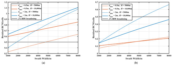
Figure 5.
Due to different jamming range swath widths, the influence of different SAR maximum trajectory offsets and flight altitudes on residual RCM are considered. (a) The azimuth resolution is 1 m; (b) The azimuth resolution is 2.5 m.
We can find that the smaller the SAR trajectory deviation and the lower the flight altitude and resolution, the easier it is for the jamming signal based on the HDE algorithm to meet the limitation of residual RCM after SAR imaging.
Next, the azimuth compression results are analyzed, only considering the exponential term in Equation (50). The inverse Fourier transform along the azimuth direction is as follows:
let , since , Equation (53) can be equivalent to:
It can be obtained from Equation (54) that the phase of the jamming signal after imaging is destroyed by the residual quadratic trajectory construction error term , which will lead to a certain degree of azimuth defocusing and sidelobe asymmetry after azimuth compression. Its influence on the azimuth main lobe broadening can be estimated by the quadratic phase error (QPE). For a typical Kaiser window of , if the required broadening is less than , the corresponding absolute value of QPE should be less than [1]. The expression of QPE is as follows:
An equivalent substitution of the QPE can be achieved through the limitation of the maximum trajectory deviation :
Figure 6 shows the HDE algorithm against different SAR maximum trajectory offsets, azimuth resolution, and jamming range swath widths quadratic phase error. For the SAR with the maximum trajectory deviation of 4 m and the false target within the jamming range width of 8000 m, the residual quadratic trajectory construction phase error is much smaller than , and the resulting defocus is negligible.
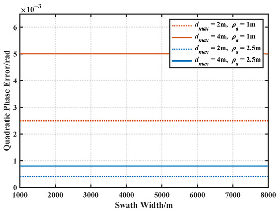
Figure 6.
Due to different jamming range swath widths, the influence of different SAR maximum trajectory offsets, and azimuth resolution on quadratic phase error are considered.
In summary, the jamming effect after imaging based on the HDE algorithm is mainly affected by the residual RCM in Equation (51). To achieve the desired deceptive jamming effect, the HDE algorithm needs to restrict the SAR flight height, azimuth resolution, and jamming range swath width according to Equation (52), which leads to the fact that the effective jamming area in the range direction does not exceed the jamming swath width. However, there are no restrictions on the effective jamming area in the azimuth direction.
As seen from Figure 5a, for the nonlinear-trajectory airborne SAR with 5000 m flight height, 1 m resolution, and 0.5 m maximum trajectory offsets, the HDE algorithm can cover the deceptive jamming with a range width of about 7 km. The restriction of the HDE algorithm on the maximum trajectory deviation is mainly referred to in Equations (40), (41), (43), (52) and (57). Equations (43) and (52) have the strictest restriction, which is essential because the establishment of jamming signal imaging analysis of the HDE algorithm above is directly influenced by the decomposition effectiveness of the function. Therefore, it can be concluded that the HDE algorithm is suitable for jamming medium-resolution airborne SAR with a slow, larger-amplitude or fast, smaller-amplitude trajectory deviation.
4. Simulation and Result
In this section, the effectiveness of the HDE algorithm is proved by simulating the jamming results of fake targets and scenes, and the algorithm’s computational complexity is analyzed. In the simulation process, the jamming signal is first generated by the jammer according to the received SAR signal, and then the SAR radar performs motion compensation imaging. The jamming object is an X-band nonlinear-trajectory SAR operating in strip mode. Table 1 shows the main parameters of the simulation. It is assumed that the radar trajectory has a trajectory deviation relative to the nominal straight trajectory. The function of the trajectory deviation in the horizontal direction is , and the function of the trajectory deviation in the vertical direction is , where denotes the uniformly distributed random variable, the maximum trajectory deviation is 0.5 m, as shown in Figure 7. The settings of the above parameters all satisfy the validity constraints of the HDE algorithm in Section 3.2.
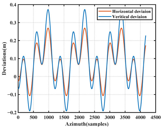
Figure 7.
SAR trajectory deviation vertical component and horizontal component.
4.1. Fake Point Scatters Simulation
To analyze the imaging quality of false target scattering points at different positions, a scatterer array with an interval of 1.5 km is set as a deceptive jamming template. As shown in Figure 8, the scattering points are numbered ∼ in order. The central point of this deceptive jamming template is set to coincide with the position of the jammer.
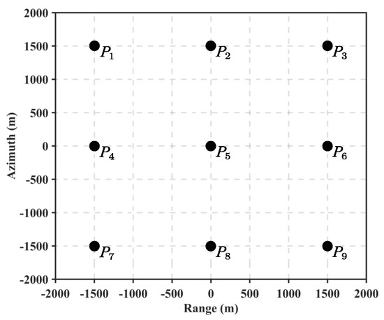
Figure 8.
Deception jamming fake target template.
First, the HDE algorithm is used to generate the deceptive jamming signal. The real scattering point (RS) echo signal and straightforward calculation algorithm (SA) deceptive jamming algorithm are compared and analyzed. RS and SA algorithms generate jamming signals in the time domain by directly obtaining nonlinear-trajectory slant-range point-by-point superposition, which is theoretically the closest to the echo signal of the actual scene. Figure 9 shows the imaging results in the side-looking strip mode, where Figure 9c is the jamming imaging result of HDE, and Figure 9a,b are the imaging results using RS and SA algorithm, respectively. These three algorithms can achieve approximately the same focusing effects from a macroscopic view of the image.
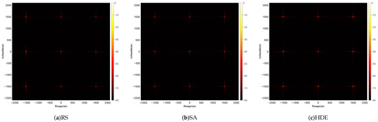
Figure 9.
Imaging results of the fake target template. (a) Real scatters; (b) and (c) Fake target generated using SA and HDE.
To analyze the focusing characteristics of the jamming signal in detail, a comparison of range and azimuth profiles of all scattering points is shown in Figure 10 and Figure 11. The solid orange and dot-dashed blue lines are the range-azimuth imaging contours of the RS and SA algorithms, respectively. The results are very similar and can be used as a reference for standard scattering points. The solid red line represents the result of the HDE algorithm. As analyzed in Section 3.2, due to the residual RCM effect, the imaging results of the jamming scattering points show a small main lobe broadening in both the range and azimuth direction.
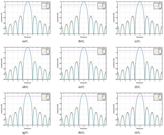
Figure 10.
Range profiles of the RS and fake scatterers generated using SA and HDE. (a–i) Range profiles of scatterers –.
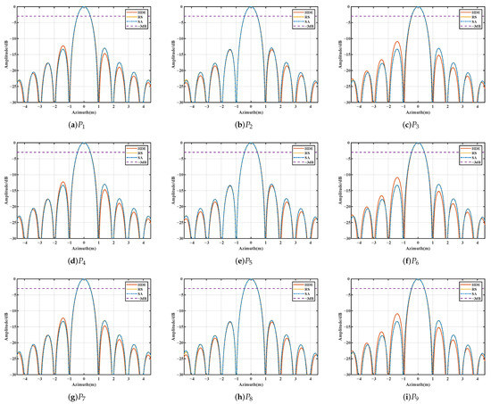
Figure 11.
Azimuth profiles of the RS and fake scatterers generated using SA and HDE. (a–i) Azimuth profiles of scatterers –.
The range and azimuth dimensions imaging quality parameters of each scattering point are given in Table 2, including 3 dB impulse response width (IRW), peak side lobe ratio (PSLR), and integral side lobe ratio (ISLR). The last two columns of Table 2 list the statistical indices of all nine scattering points, including mean and standard deviation. It can be concluded from the table that the IRW in the range and azimuth directions measured by RS is 0.88 m and 0.87 m, respectively. In the range direction, the maximum IRWB of the false scattering points generated by the HDE algorithm is 0.67%. In the azimuth direction, the maximum IRW broadening (IRWB) of the HDE algorithm is 0.55%.
Table 2.
Imaging quality indexes comparison of different algorithms.
4.2. General Deceptive Scene Case
In this section, the HDE algorithm is applied to generate an extended fake scene. The jamming object is a nonlinear SAR with the trajectory deviation shown in Figure 7 and its parameters shown in Table 1. The deceptive template is constructed based on the SAR image acquired by TerraSAR-X in the spotlight SAR mode [37], which can take advantage of the large scene, sharp contrast, and high-resolution characteristics of the image in this mode To compare and illustrate the focusing ability of the algorithm. First, the HDE algorithm is used to generate the same fake scene as the deceptive jamming template for comparison to evaluate the jamming effect. The imaging processing of the interfering signal does not involve the actual echoes of the scene. The actual scene generated by the RS and the fake scene image generated by the HDE algorithm, as shown in Figure 12 and Figure 13.
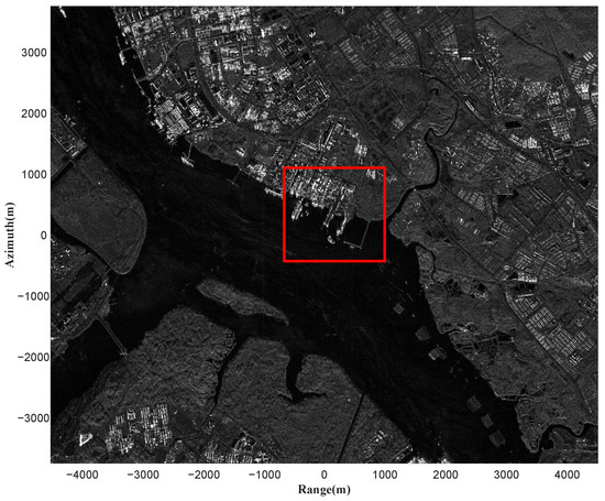
Figure 12.
Actual scene generated using RS. Parts of the image marked by rectangular red box is enlarged and shown in Figure 14a.

Figure 13.
Fake scene generated using HDE. Parts of the image marked by rectangular red box is enlarged and shown in Figure 14b.
From the overall views of the radar image, the jamming image of the HDE algorithm is approximately consistent with the original SAR image. To find out the difference in details, the 1500 m × 1800 m area shown in the red box is enlarged, i.e., Figure 14a,b, and the structural similarity SSIM is used to measure the difference between the two images and evaluate the quality of jamming radar image. The measured value of structural similarity (SSIM) is 0.95, indicating that the jamming image of the HDE algorithm is very similar to the original SAR image. The results show that the HDE algorithm can well preserve the deceptive electromagnetic features such as false scene points, lines, surfaces, and brightness when jamming nonlinear-trajectory SAR.
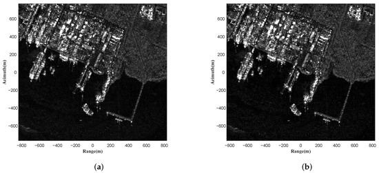
Figure 14.
Partial enlargement in red boxes. (a) Actual scene generated using RS; (b) Fake scene generated using HDE.
Then deceptive jamming templates for islands and ship groups are obtained from other SAR images with sizes of 2500 m × 2000 m and 2000 m × 3500 m, respectively. In addition, the jamming signal is generated by the HDE algorithm to jam the actual coastal scene in Figure 15a. Figure 15b shows the result of jamming imaging, with fake islands and groups of ships set beyond the coastline. Compared with the actual scene in Figure 15a, the fake pier scene is well-focused and difficult to distinguish from the actual scene. The results verify the effectiveness of the proposed algorithm.
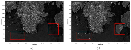
Figure 15.
Fake scene deceptive jamming simulation. (a) Imaging result of the actual scene echo, parts of the actual image marked by rectangular red box; (b) Imaging result after adding the jamming signal to the echo by HDE, parts of the jamming image marked by rectangular red box.
4.3. Computational Complexity Analysis
In this section, the computational complexity of the HDE algorithm will be estimated to evaluate its practical value. For ease of analysis, those operations used in the algorithm in Section 2.3.2, such as addition, multiplication, and square root, are considered basic operations that can be performed by the floating-point unit in one instruction cycle. We assume that the jamming scene template consists of point scatterers, where the number of azimuth cells is M and the number of range cells is N. The following part will analyze the number of basic operations of jamming modulation under a specific number of range sampling points and azimuth sampling points .
In the initialization stage, for a scattering point , calculating the slant range requires seven basic operations. Since the complex number calculation completes the nominal slant range phase compensation, the basic operation amount is 5, and the azimuth FFT requires basic operations. Therefore, the basic operation of is needed to complete the azimuth time–frequency conversion of the deceptive jamming template. requires basic operations. Therefore, combined with the azimuth inverse Fourier transform, the basic operation amount in the initialization stage is:
In the real-time calculation stage, the components of the trajectory deviation need to be calculated in each PRI period, and the basic operation amount of and is . Completing the construction of and is requires a total of basic operations, and the range FFT requires basic operations. Therefore, the basic operations of are required to complete the JSF operation of a PRI in the real-time computation stage, and the basic operation amount of convolutional forwarding modulation combined with DRFM is:
From the above analysis, the characteristics of the HDE algorithm can be summarized. The main calculation amount of the HDE algorithm is the Fourier transform, whether it is the initialization stage or the real-time calculation stage. In addition, the construction for nonlinear-trajectory in the real-time stage can be accomplished simply by complex multiplication. Similarly, the basic operation amount of the traditional deceptive jamming SA algorithm for nonlinear-trajectory SAR is analyzed, which is listed in Table 3.
Table 3.
Basic operation amount comparison of different algorithms.
If the nonlinear-trajectory jamming modulation characteristics are not discussed, only the calculation efficiency of the algorithm is considered. In Table 3, the basic operation amount of the linear trajectory SAR efficient deceptive jamming algorithm, the spatial frequency-domain interpolation (SFI) [23] algorithm and the segmented modulation (SM) [14] algorithm are supplemented.
To observe the comparison between the computational complexity of these algorithms more clearly, control , and draw the logarithmic graph of each algorithm’s total and real-time operation amount, as shown in Figure 16. It can be seen that the operation amount of the HDE algorithm is lower than the SA algorithm in the whole jamming modulation process or the real-time calculation stage. In particular, the real-time calculation of the HDE algorithm only requires complex multiplication and Fourier transform. Compared with the two-dimensional interpolation operation of the SFI algorithm and SM algorithm, the calculation efficiency is higher, and the real-time operation amount is reduced by more than .
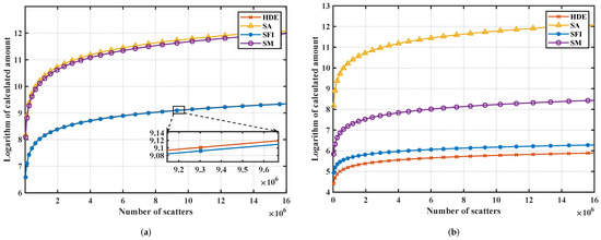
Figure 16.
The relationship between the operation amount and the total number of scatters in the template. (a) is the total operation amount and (b) is the operation amount in the real-time calculation stage.
The average running time simulation experiment was carried out on a computer with AMD PRO 5975WX CPU (main frequency: 3.6 GHz). In addition, the simulation parameters are shown in Table 1, , . We used Matlab2021a to simulate the two nonlinear-trajectory SAR deceptive jamming algorithms and calculated the average running times under different template sizes, as given in Table 4.
Table 4.
Average Running Time of The Nonlinear Deceptive Jamming Algorithms.
It is further verified that the HDE algorithm has the characteristics of the deceptive jamming algorithm in the azimuth frequency domain, and its real-time calculation complexity has nothing to do with the template size, and is far superior to the SA algorithm. In addition, the simulation time results do not perfectly match the theoretical analysis, as MATLAB uses different degrees of optimization algorithms for different calculations. In addition, the MATLAB interpreter is less efficient, and simulation times are relatively long. If field-programmable gate arrays or digital signal processors are used, the processing speed can be increased by more than tens of times, and the real-time requirements are guaranteed.
In the implementation of SAR jamming, the jammer must complete all operations within each PRI, and the calculation complexity of the real-time stage is particularly important. Based on the above analysis, the calculation complexity of the HDE algorithm is more advantageous than other algorithms, and it is more conducive to the deceptive jamming of large false scenes for nonlinear-trajectory SAR.
5. Discussion
According to the validity analysis of the HDE deceptive jamming algorithm in Section 3.2, the algorithm assumes beam center approximation and the decomposition of , which will lead to the residual RCM and quadratic phase error after imaging processing. However, the imaging quality of HDE deceptive jamming can be guaranteed by limiting the maximum trajectory deviation by Equation (43). Combining the constraints of Equations (43), (52) and (57), the following conclusions can be drawn for the HDE algorithm.
- The range imaging quality of the fake point target is related to the fake target point’s slant-range length . As becomes longer, the range broadening of the target will become larger.
- The azimuth imaging quality of the fake target is related to the slant-range length and trajectory deviation of the fake target. As becomes longer, the azimuth broadening of the fake target will become larger. As the trajectory deviation becomes larger, the peak sidelobe ratio PSLR in the azimuth direction will become higher, and the sidelobes will be asymmetrical.
These phenomena can be seen in Table 2. The range and azimuth broadening of ∼ increase with the increase of the target slant range, which is caused by the residual RCM with the increase of the target slant range. At the same time, the residual RCM also causes the main lobe position of each point to shift slightly in the range direction and azimuth direction. Due to the influence of the quadratic sinusoidal phase error, there will be asymmetry of the side lobe and distortion of the main lobe at each point in the azimuth direction, which makes the deviation of the main lobe in the azimuth direction larger than that in the range direction. However, the maximum IRW broadening in Table 2 does not exceed 0.7%, the maximum main lobe offset does not exceed 0.5 range resolution cells, and has almost no effect on the fake scene imaging in Figure 13, Figure 14 and Figure 15. In summary, the imaging quality of the deceptive jamming of the HDE algorithm can be guaranteed.
According to the analysis in Section 4.3, the HDE algorithm has significant advantages over other deceptive jamming algorithms in terms of computational complexity. This is because the azimuth time–frequency hybrid domain modulation in the HDE algorithm significantly improves computational efficiency and flexibility, making nonlinear-trajectory deceptive jamming more feasible. It should be noted that the jamming target of the HDE algorithm is not limited to nonlinear-trajectory SAR, and it can also jam linear trajectory SAR. However, the proposed HDE algorithm still has certain problems. For example, the algorithm has yet to be extended to adapt to squint SAR, spaceborne SAR, and other SAR working modes. These are issues that we need to study further in the future.
6. Conclusions
This paper mainly studies the deceptive jamming problem of nonlinear-trajectory SAR and proposes a nonlinear-trajectory SAR deceptive jamming algorithm based on hybrid domain efficient modulation. The HDE algorithm calculates the JFR of linear trajectory in the azimuth frequency domain and performs real-time trajectory deviation construction in the azimuth time domain. The characteristic of this algorithm is that it can generate JFR by constructing the trajectory deviation pulse-by-pulse in the azimuth time domain, which makes it especially suitable for deceptive jamming against nonlinear-trajectory SAR. In the initialization and real-time computation stages, the HDE algorithm only uses Fourier transform and complex multiplication operations, balancing computational efficiency and modulation flexibility. Additionally, we have summarized the validity constraints of the HDE algorithm implementation. The simulation and complexity analysis results indicate that, compared to the traditional SA algorithm, the HDE algorithm has a significant computational complexity advantage while ensuring the jamming signals’ focusing ability. The HDE algorithm provides a new solution for the deceptive jamming problem of nonlinear-trajectory SAR, with the potential for practical application in SAR jamming. In the future, we will continue to study and extend this algorithm to more SAR imaging modes.
Author Contributions
Conceptualization, J.D., Q.Z. and W.L.; Data curation, J.D.; Formal analysis, J.D. and Q.Z.; Funding acquisition, Q.Z. and W.L.; Investigation, J.D. and W.C.; Methodology, J.D. and W.C.; Project administration, Q.Z. and X.L.; Resources, J.D. and Q.Z.; Software, J.D.; Supervision, Q.Z. and X.L.; Validation, J.D.; Visualization, J.D.; Writing—original draft, J.D.; Writing—review and editing, J.D. and Q.Z. All authors have read and agreed to the published version of the manuscript.
Funding
This work was funded by the Stable-Support Scientific Project of China Research Institute of Radiowave Propagation (No. A132003W02).
Data Availability Statement
Not applicable.
Conflicts of Interest
The authors declare no conflict of interest.
References
- Cumming, I.G.; Wong, F.H. Digital Processing Of Synthetic Aperture Radar Data; Artech House Publishers: Boston, MA, USA, 2005; pp. 473–476. [Google Scholar]
- Condley, C. Some System Considerations for Electronic Countermeasures to Synthetic Aperture Radar. In Proceedings of the IEE Colloquium on Electronic Warfare Systems, London, UK, 14 January 1991; pp. 8/1–8/7. [Google Scholar]
- Dumper, K.; Cooper, P.; Wons, A.; Condley, C.; Tully, P. Spaceborne Synthetic Aperture Radar and Noise Jamming. In Proceedings of the Radar 97 (Conf. Publ. No. 449), Edinburgh, UK, 14–16 October 1997; pp. 411–414. [Google Scholar] [CrossRef]
- Fouts, D.J.; Pace, P.E.; Karow, C.; Ekestorm, S. A Single-Chip False Target Radar Image Generator for Countering Wideband Imaging Radars. IEEE J.-Solid-State Circuits 2002, 37, 751–759. [Google Scholar] [CrossRef]
- Lee, Y.; Park, J.; Shin, W.; Lee, K.; Kang, H. A Study on Jamming Performance Evaluation of Noise and Deception Jammer against SAR Satellite. In Proceedings of the 2011 3rd International Asia-Pacific Conference on Synthetic Aperture Radar (APSAR), Seoul, Republic of Korea, 26–30 September 2011; pp. 1–3. [Google Scholar]
- Ye, W.; Ruan, H.; Zhang, S.x.; Yan, L. Study of Noise Jamming Based on Convolution Modulation to SAR. In Proceedings of the 2010 International Conference on Computer, Mechatronics, Control and Electronic Engineering, Changchun, China, 24–26 August 2010; Volume 6, pp. 169–172. [Google Scholar] [CrossRef]
- Garmatyuk, D.; Narayanan, R. ECCM Capabilities of an Ultrawideband Bandlimited Random Noise Imaging Radar. IEEE Trans. Aerosp. Electron. Syst. 2002, 38, 1243–1255. [Google Scholar] [CrossRef]
- Song, C.; Wang, Y.; Jin, G.; Wang, Y.; Dong, Q.; Wang, B.; Zhou, L.; Lu, P.; Wu, Y. A Novel Jamming Method against SAR Using Nonlinear Frequency Modulation Waveform with Very High Sidelobes. Remote Sens. 2022, 14, 5370. [Google Scholar] [CrossRef]
- Cheng, D.; Liu, Z.; Guo, Z.; Shu, G.; Li, N. A Repeater-Type SAR Deceptive Jamming Method Based on Joint Encoding of Amplitude and Phase in the Intra-Pulse and Inter-Pulse. Remote Sens. 2022, 14, 4597. [Google Scholar] [CrossRef]
- Wang, S.; Li, Y.U.; Jin, N.I.; Zhang, G. A Study on the Active Deception Jamming to SAR. Acta Electron. Sin. 2003, 31, 1900–1902. [Google Scholar]
- Yan, Z.; Guoqing, Z.; Yu, Z. Research on SAR Jamming Technique Based on Man-made Map. In Proceedings of the 2006 CIE International Conference on Radar, Shanghai, China, 16–19 October 2006; pp. 1–4. [Google Scholar] [CrossRef]
- Lin, X.; Liu, P.; Xue, G. Fast Generation of SAR Deceptive Jamming Signal Based on Inverse Range Doppler Algorithm. In Proceedings of the IET International Radar Conference 2013, Xi’an, China, 14–16 April 2013; pp. 1–4. [Google Scholar] [CrossRef]
- He, X.; Zhu, J.; Wang, J.; Du, D.; Tang, B. False Target Deceptive Jamming for Countering Missile-Borne SAR. In Proceedings of the 2014 IEEE 17th International Conference on Computational Science and Engineering, Chengdu, China, 19–21 December 2014; pp. 1974–1978. [Google Scholar] [CrossRef]
- Zhou, F.; Zhao, B.; Tao, M.; Bai, X.; Chen, B.; Sun, G. A Large Scene Deceptive Jamming Method for Space-Borne SAR. IEEE Trans. Geosci. Remote Sens. 2013, 51, 4486–4495. [Google Scholar] [CrossRef]
- Sun, Q.; Shu, T.; Zhou, S.; Tang, B.; Yu, W. A Novel Jamming Signal Generation Method for Deceptive SAR Jammer. In Proceedings of the 2014 IEEE Radar Conference, Cincinnati, OH, USA, 19–23 May 2014; pp. 1174–1178. [Google Scholar] [CrossRef]
- Zhao, B.; Zhou, F.; Bao, Z. Deception Jamming for Squint SAR Based on Multiple Receivers. IEEE J. Sel. Top. Appl. Earth Obs. Remote Sens. 2015, 8, 3988–3998. [Google Scholar] [CrossRef]
- Zhao, B.; Huang, L.; Zhou, F.; Zhang, J. Performance Improvement of Deception Jamming Against SAR Based on Minimum Condition Number. IEEE J. Sel. Top. Appl. Earth Obs. Remote Sens. 2017, 10, 1039–1055. [Google Scholar] [CrossRef]
- Sun, Q.; Shu, T.; Yu, K.B.; Yu, W. Efficient Deceptive Jamming Method of Static and Moving Targets Against SAR. IEEE Sens. J. 2018, 18, 3610–3618. [Google Scholar] [CrossRef]
- Liu, Y.; Wei, W.; Pan, X.; Dai, D.; Feng, D. A Frequency-Domain Three-Stage Algorithm for Active Deception Jamming against Synthetic Aperture Radar. IET Radar Sonar Navig. 2014, 8, 639–646. [Google Scholar] [CrossRef]
- Liu, Y.; Wang, W.; Pan, X.; Fu, Q.; Wang, G. Inverse Omega-K Algorithm for the Electromagnetic Deception of Synthetic Aperture Radar. IEEE J. Sel. Top. Appl. Earth Obs. Remote Sens. 2016, 9, 3037–3049. [Google Scholar] [CrossRef]
- Zhao, B.; Huang, L.; Li, J.; Liu, M.; Wang, J. Deceptive SAR Jamming Based on 1-Bit Sampling and Time-Varying Thresholds. IEEE J. Sel. Top. Appl. Earth Obs. Remote Sens. 2018, 11, 939–950. [Google Scholar] [CrossRef]
- Yang, K.; Ye, W.; Ma, F.; Li, G.; Tong, Q. A Large-Scene Deceptive Jamming Method for Space-Borne SAR Based on Time-Delay and Frequency-Shift with Template Segmentation. Remote Sens. 2019, 12, 53. [Google Scholar] [CrossRef]
- Yang, K.; Ma, F.; Ran, D.; Ye, W.; Li, G. Fast Generation of Deceptive Jamming Signal Against Spaceborne SAR Based on Spatial Frequency Domain Interpolation. IEEE Trans. Geosci. Remote Sens. 2022, 60, 1–15. [Google Scholar] [CrossRef]
- Lee, H.; Kim, K.W. An Integrated Raw Data Simulator for Airborne Spotlight ECCM SAR. Remote Sens. 2022, 14, 3897. [Google Scholar] [CrossRef]
- Shenghua, Z.; Dazhuan, X.; Xueming, J.; Hua, H. A Study on Active Jamming to Synthetic Aperture Radar. In Proceedings of the ICCEA 2004. 2004 3rd International Conference on Computational Electromagnetics and Its Applications, Beijing, China, 1–4 November 2004; pp. 403–406. [Google Scholar] [CrossRef]
- Dai, D.h.; Wu, X.F.; Wang, X.s.; Xiao, S.p. SAR Active-Decoys Jamming Based on DRFM. In Proceedings of the 2007 IET International Conference on Radar Systems, Edinburgh, UK, 15–18 October 2007; pp. 1–4. [Google Scholar]
- Sun, G.; Jiang, X.; Xing, M.; Qiao, Z.j.; Wu, Y.; Bao, Z. Focus Improvement of Highly Squinted Data Based on Azimuth Nonlinear Scaling. IEEE Trans. Geosci. Remote Sens. 2011, 49, 2308–2322. [Google Scholar] [CrossRef]
- Yi, T.; He, Z.; He, F.; Dong, Z.; Wu, M. Generalized Nonlinear Chirp Scaling Algorithm for High-Resolution Highly Squint SAR Imaging. Sensors 2017, 17, 2568. [Google Scholar] [CrossRef]
- Fornado, G. Trajectory Deviations in Airborne SAR: Analysis and Compensation. IEEE Trans. Aerosp. Electron. Syst. 1999, 35, 997–1009. [Google Scholar] [CrossRef]
- Guo, H.; Li, Y.; Qu, Q.; Liu, P. Studying Atmospheric Turbulence Effects on Aircraft Motion for Airborne SAR Motion Compensation Requirements. In Proceedings of the 2012 IEEE International Conference on Imaging Systems and Techniques Proceedings, Manchester, UK, 16–17 July 2012; pp. 152–157. [Google Scholar] [CrossRef]
- Mao, Y.; Xiang, M.; Wei, L.; Li, Y.; Hong, W. Error Analysis of SAR Motion Compensation. In Proceedings of the 2012 IEEE International Conference on Imaging Systems and Techniques Proceedings, Manchester, UK, 16–17 July 2012; pp. 377–380. [Google Scholar] [CrossRef]
- Perna, S.; Zamparelli, V.; Pauciullo, A.; Fornaro, G. Azimuth-to-Frequency Mapping in Airborne SAR Data Corrupted by Uncompensated Motion Errors. IEEE Geosci. Remote Sens. Lett. 2013, 10, 1493–1497. [Google Scholar] [CrossRef]
- Franceschetti, G.; Iodice, A.; Perna, S.; Riccio, D. SAR Sensor Trajectory Deviations: Fourier Domain Formulation and Extended Scene Simulation of Raw Signal. IEEE Trans. Geosci. Remote Sens. 2006, 44, 2323–2334. [Google Scholar] [CrossRef]
- Franceschetti, G.; Iodice, A.; Perna, S.; Riccio, D. Efficient Simulation of Airborne SAR Raw Data of Extended Scenes. IEEE Trans. Geosci. Remote Sens. 2006, 44, 2851–2860. [Google Scholar] [CrossRef]
- Proakis, J.G.; Salehi, M.; Zhou, N.; Li, X. Communication Systems Engineering; Prentice Hall: Hoboken, NJ, USA, 1994; Volume 2. [Google Scholar]
- Fornaro, G.; Franceschetti, G.; Perna, S. Motion Compensation Errors: Effects on the Accuracy of Airborne SAR Images. IEEE Trans. Aerosp. Electron. Syst. 2005, 41, 1338–1352. [Google Scholar] [CrossRef]
- Sample Imagery Detail. Available online: https://www.intelligence-airbusds.com (accessed on 13 November 2022).
Disclaimer/Publisher’s Note: The statements, opinions and data contained in all publications are solely those of the individual author(s) and contributor(s) and not of MDPI and/or the editor(s). MDPI and/or the editor(s) disclaim responsibility for any injury to people or property resulting from any ideas, methods, instructions or products referred to in the content. |
© 2023 by the authors. Licensee MDPI, Basel, Switzerland. This article is an open access article distributed under the terms and conditions of the Creative Commons Attribution (CC BY) license (https://creativecommons.org/licenses/by/4.0/).