
Fine Resolution Classification of New Ice, Young Ice, and First-Year Ice Based on Feature Selection from Gaofen-3 Quad-Polarization SAR

 ,
,  , ,
, ,
Abstract

1. Introduction
2. Dataset
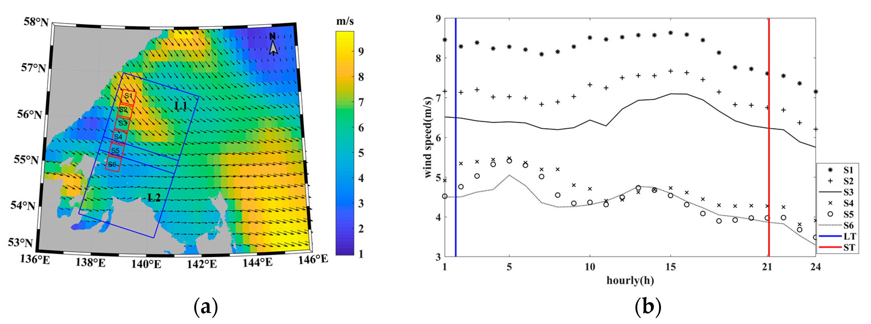
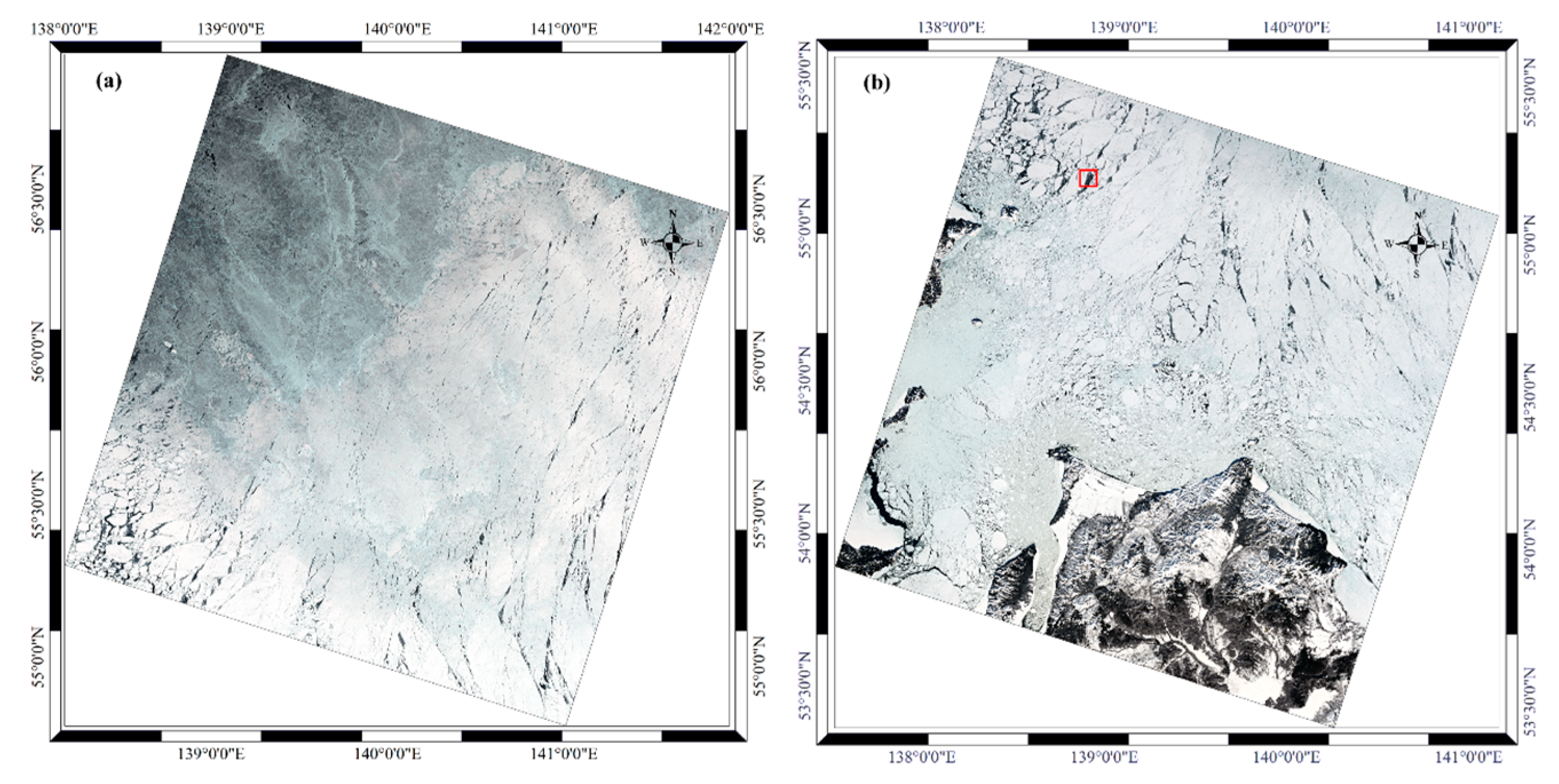
2.1. Landsat-8
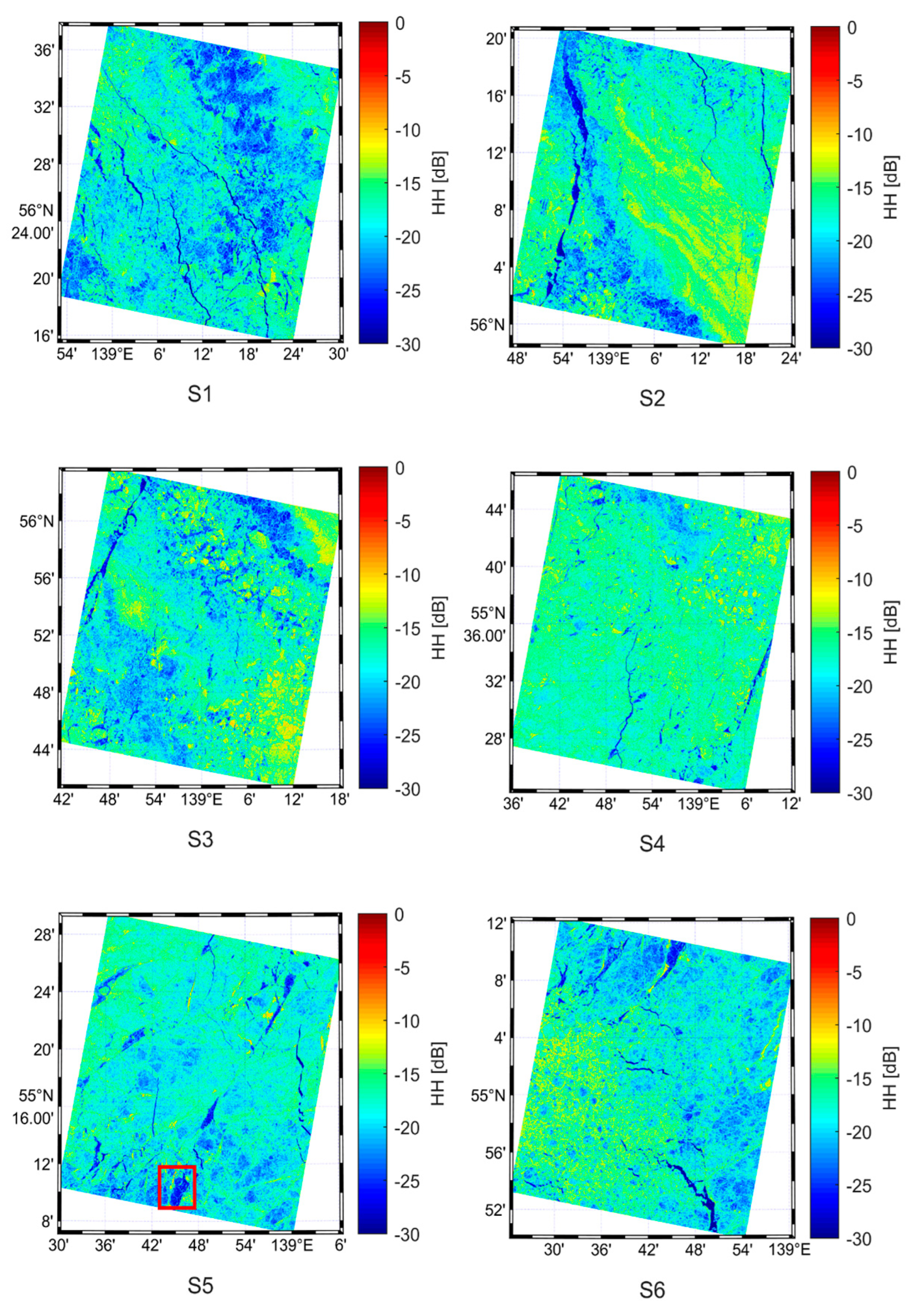
2.2. GF-3 SAR Images
3. SAR Parameters
3.1. Quad-Pol SAR Parameters
3.2. Hybrid-Pol SAR Parameters
4. Methods
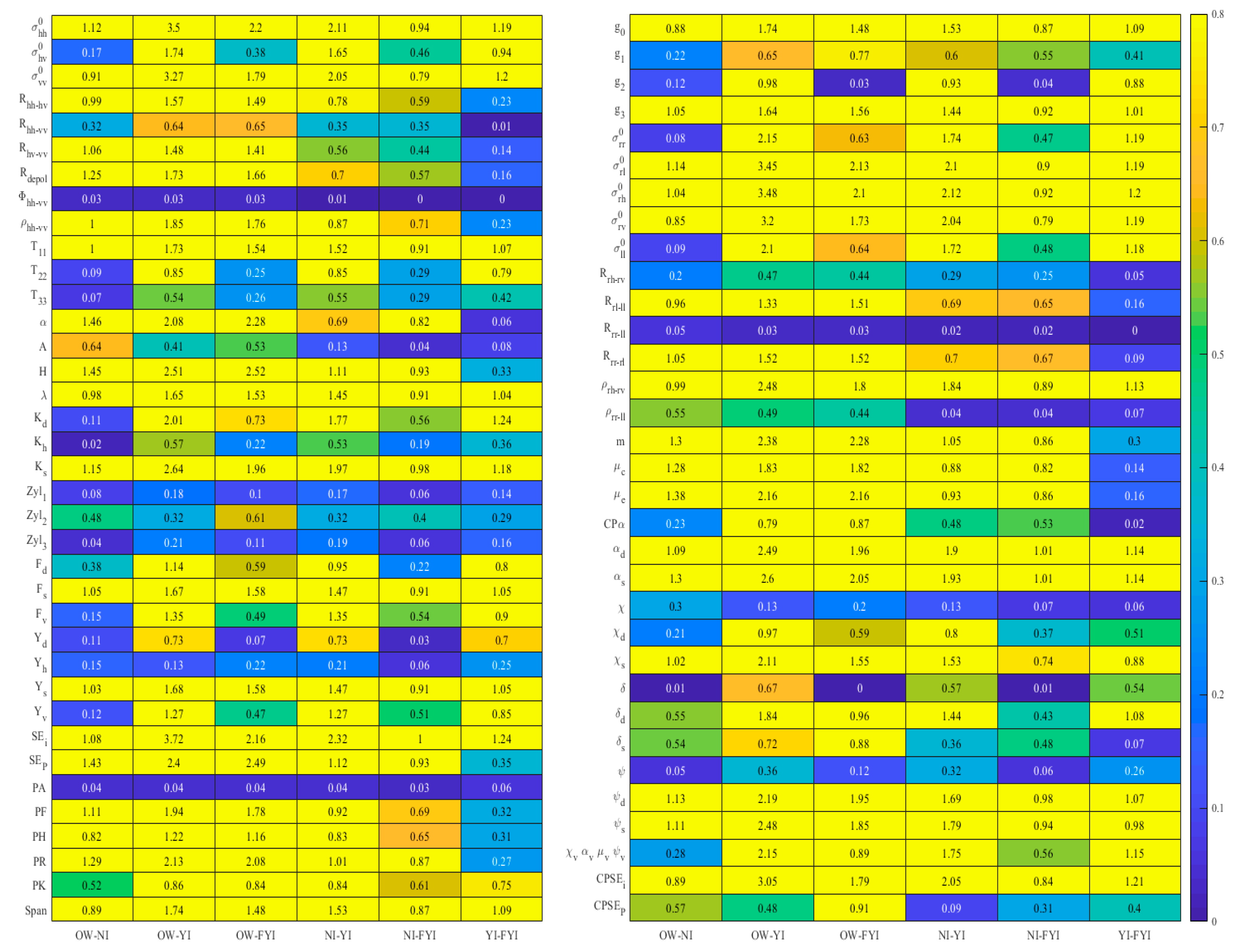
4.1. Separability Index (SI)
4.2. Parameters Selection
- Co-pol intensity parameters (, T11),
- Total power parameters (, SEi, Span),
- Parameters that indicate surface scattering (Fs, Ys, Ks).
- 4.
- Circle-polarized intensity parameters (g3, , , ) whose dominant scattering is surface scattering,
- 5.
- Total power parameters (g0, CPSEi), which are similar to the corresponding quad-pol,
- 6.
- Depolarization parameters () due to multi-scattering
- 7.
- Parameters representing the orientation and polarization angle (, , , ).
4.3. Random Forest Classifier
5. Results
5.1. Classification Results
5.2. Verification
6. Discussion
7. Conclusions
Author Contributions
Funding
Data Availability Statement
Acknowledgments
Conflicts of Interest
References
- Wunderling, N.; Willeit, M.; Donges, J.F.; Winkelmann, R. Global Warming Due to Loss of Large Ice Masses and Arctic Summer Sea Ice. Nat. Commun. 2020, 11, 5177. [Google Scholar] [CrossRef]
- Nghiem, S.V.; Rigor, I.G.; Perovich, D.K.; Clemente-Colón, P.; Weatherly, J.W.; Neumann, G. Rapid Reduction of Arctic Perennial Sea Ice. Geophys. Res. Lett. 2007, 34, L19504. [Google Scholar] [CrossRef]
- Perovich, D.K.; Polashenski, C. Albedo Evolution of Seasonal Arctic Sea Ice. Geophys. Res. Lett. 2012, 39, L08501. [Google Scholar] [CrossRef]
- Pegau, W.S.; Paulson, C.A. The Albedo of Arctic Leads in Summer. Ann. Glaciol. 2001, 33, 221–224. [Google Scholar] [CrossRef]
- Kurtz, N.T.; Markus, T.; Farrell, S.L.; Worthen, D.L.; Boisvert, L.N. Observations of Recent Arctic Sea Ice Volume Loss and Its Impact on Ocean-Atmosphere Energy Exchange and Ice Production. J. Geophys. Res. 2011, 116, C04015. [Google Scholar] [CrossRef]
- Else, B.G.T.; Papakyriakou, T.N.; Raddatz, R.; Galley, R.J.; Mundy, C.J.; Barber, D.G.; Swystun, K.; Rysgaard, S. Surface Energy Budget of Landfast Sea Ice during the Transitions from Winter to Snowmelt and Melt Pond Onset: The Importance of Net Longwave Radiation and Cyclone Forcings. J. Geophys. Res. Ocean. 2014, 119, 3679–3693. [Google Scholar] [CrossRef]
- Kwok, R.; Spreen, G.; Pang, S. Arctic Sea Ice Circulation and Drift Speed: Decadal Trends and Ocean Currents: Arctic Sea Ice Motion. J. Geophys. Res. Ocean. 2013, 118, 2408–2425. [Google Scholar] [CrossRef]
- Roy, F.; Chevallier, M.; Smith, G.C.; Dupont, F.; Garric, G.; Lemieux, J.; Lu, Y.; Davidson, F. Arctic Sea Ice and Freshwater Sensitivity to the Treatment of the Atmosphere-ice-ocean Surface Layer. J. Geophys. Res. Ocean. 2015, 120, 4392–4417. [Google Scholar] [CrossRef]
- Stroeve, J.; Holland, M.M.; Meier, W.; Scambos, T.; Serreze, M. Arctic Sea Ice Decline: Faster than Forecast: Arctic Ice Loss-Faster than Forecast. Geophys. Res. Lett. 2007, 34, L09501. [Google Scholar] [CrossRef]
- Martin, T.; Tsamados, M.; Schroeder, D.; Feltham, D.L. The Impact of Variable Sea Ice Roughness on Changes in Arctic Ocean Surface Stress: A Model Study. J. Geophys. Res. Ocean. 2016, 121, 1931–1952. [Google Scholar] [CrossRef]
- Zakhvatkina, N.; Smirnov, V.; Bychkova, I. Satellite SAR Data-Based Sea Ice Classification: An Overview. Geosciences 2019, 9, 152. [Google Scholar] [CrossRef]
- Moen, M.-A.N.; Anfinsen, S.N.; Doulgeris, A.P.; Renner, A.H.H. Gerland Assessing Polarimetric SAR Sea-Ice Classifications Using Consecutive Day Images. Ann. Glaciol. 2015, 56, 285–294. [Google Scholar] [CrossRef]
- Li, X.-M.; Sun, Y.; Zhang, Q. Extraction of Sea Ice Cover by Sentinel-1 SAR Based on Support Vector Machine with Unsupervised Generation of Training Data. IEEE Trans. Geosci. Remote Sens. 2021, 59, 3040–3053. [Google Scholar] [CrossRef]
- Wang, Y.-R.; Li, X.-M. Arctic Sea Ice Cover Data From Spaceborne Synthetic Aperture Radar by Deep Learning. Earth Syst. Sci. Data 2021, 13, 2723–2742. [Google Scholar] [CrossRef]
- Liu, H.; Guo, H.; Zhang, L. SVM-Based Sea Ice Classification Using Textural Features and Concentration From RADARSAT-2 Dual-Pol ScanSAR Data. IEEE J. Sel. Top. Appl. Earth Obs. Remote Sens. 2015, 8, 1601–1613. [Google Scholar] [CrossRef]
- Espeseth, M.; Brekke, C.; Johansson, A. Assessment of RISAT-1 and Radarsat-2 for Sea Ice Observations from a Hybrid-Polarity Perspective. Remote Sens. 2017, 9, 1088. [Google Scholar] [CrossRef]
- Raney, R.K. Hybrid-Polarity SAR Architecture. IEEE Trans. Geosci. Remote Sens. 2007, 45, 3397–3404. [Google Scholar] [CrossRef]
- Souyris, J.-C.; Imbo, P.; Fjortoft, R.; Mingot, S.; Lee, J.-S. Compact Polarimetry Based on Symmetry Properties of Geophysical Media: The /Spl Pi//4 Mode. IEEE Trans. Geosci. Remote Sens. 2005, 43, 634–646. [Google Scholar] [CrossRef]
- Li, H.; Perrie, W. Sea Ice Characterization and Classification Using Hybrid Polarimetry SAR. IEEE J. Sel. Top. Appl. Earth Obs. Remote Sens. 2016, 9, 4998–5010. [Google Scholar] [CrossRef]
- Xie, L.; Zhang, H.; Li, H.; Wang, C. A Unified Framework for Crop Classification in Southern China Using Fully Polarimetric, Dual Polarimetric, and Compact Polarimetric SAR Data. Int. J. Remote Sens. 2015, 36, 3798–3818. [Google Scholar] [CrossRef]
- Zhang, X.; Zhang, J.; Liu, M.; Meng, J. Assessment of C-Band Compact Polarimetry SAR for Sea Ice Classification. Acta Oceanol. Sin. 2016, 35, 79–88. [Google Scholar] [CrossRef]
- Dabboor, M.; Geldsetzer, T. Towards Sea Ice Classification Using Simulated RADARSAT Constellation Mission Compact Polarimetric SAR Imagery. Remote Sens. Environ. 2014, 140, 189–195. [Google Scholar] [CrossRef]
- Singha, S.; Ressel, R. Arctic Sea Ice Characterization Using RISAT-1 Compact-Pol SAR Imagery and Feature Evaluation: A Case Study Over Northeast Greenland. IEEE J. Sel. Top. Appl. Earth Obs. Remote Sens. 2017, 10, 3504–3514. [Google Scholar] [CrossRef]
- Nasonova, S.; Scharien, R.K.; Geldsetzer, T.; Howell, S.E.L.; Power, D. Optimal Compact Polarimetric Parameters and Texture Features for Discriminating Sea Ice Types during Winter and Advanced Melt. Can. J. Remote Sens. 2018, 44, 390–411. [Google Scholar] [CrossRef]
- Shokr, M.E.; Jessup, R.; Ramsay, B. An Interactive Algorithm for Derivation of Sea Ice Classifications and Concentrations from SAR Images. Can. J. Remote Sens. 1999, 25, 70–79. [Google Scholar] [CrossRef]
- Xie, T.; Perrie, W.; Wei, C.; Zhao, L. Discrimination of Open Water from Sea Ice in the Labrador Sea Using Quad-Polarized Synthetic Aperture Radar. Remote Sens. Environ. 2020, 247, 111948. [Google Scholar] [CrossRef]
- De Abreu, R.; Flett, D.; Scheuchl, B.; Ramsay, B. Operational Sea Ice Monitoring with RADARSAT-2—A Glimpse into the Future. In Proceedings of the IGARSS 2003, 2003 IEEE International Geoscience and Remote Sensing Symposium, Toulouse, France, 21–25 July 2003; Proceedings (IEEE Cat. No.03CH37477). IEEE: Toulouse, France, 2003; Volume 2, pp. 1308–1310. [Google Scholar]
- Nystuen, J.A.; Garcia, F.W. Sea Ice Classification Using SAR Backscatter Statistics. IEEE Trans. Geosci. Remote Sens. 1992, 30, 502–509. [Google Scholar] [CrossRef]
- Partington, K.C.; Flach, J.D.; Barber, D.; Isleifson, D.; Meadows, P.J.; Verlaan, P. Dual-Polarization C-Band Radar Observations of Sea Ice in the Amundsen Gulf. IEEE Trans. Geosci. Remote Sens. 2010, 48, 2685–2691. [Google Scholar] [CrossRef]
- Zhang, J.; Zhang, W.; Hu, Y.; Chu, Q.; Liu, L. An Improved Sea Ice Classification Algorithm with Gaofen-3 Dual-Polarization SAR Data Based on Deep Convolutional Neural Networks. Remote Sens. 2022, 14, 906. [Google Scholar] [CrossRef]
- Ressel, R.; Singha, S.; Lehner, S.; Rosel, A.; Spreen, G. Investigation into Different Polarimetric Features for Sea Ice Classification Using X-Band Synthetic Aperture Radar. IEEE J. Sel. Top. Appl. Earth Obs. Remote Sens. 2016, 9, 3131–3143. [Google Scholar] [CrossRef]
- Scheuchl, B.; Flett, D.; Caves, R.; Cumming, I. Potential of RADARSAT-2 Data for Operational Sea Ice Monitoring. Can. J. Remote Sens. 2004, 30, 448–461. [Google Scholar] [CrossRef]
- Singha, S.; Johansson, M.; Hughes, N.; Hvidegaard, S.M.; Skourup, H. Arctic Sea Ice Characterization Using Spaceborne Fully Polarimetric L-, C-, and X-Band SAR With Validation by Airborne Measurements. IEEE Trans. Geosci. Remote Sens. 2018, 56, 3715–3734. [Google Scholar] [CrossRef]
- Wakabayashi, H.; Matsuoka, T.; Nakamura, K.; Nishio, F. Polarimetric Characteristics of Sea Ice in the Sea of Okhotsk Observed by Airborne L-Band SAR. IEEE Trans. Geosci. Remote Sens. 2004, 42, 2412–2425. [Google Scholar] [CrossRef]
- Zhang, X.; Dierking, W.; Zhang, J.; Meng, J. A Polarimetric Decomposition Method for Ice in the Bohai Sea Using C-Band PolSAR Data. IEEE J. Sel. Top. Appl. Earth Obs. Remote Sens. 2015, 8, 47–66. [Google Scholar] [CrossRef]
- Bi, H.; Liang, Y.; Wang, Y.; Liang, X.; Zhang, Z.; Du, T.; Yu, Q.; Huang, J.; Kong, M.; Huang, H. Arctic Multiyear Sea Ice Variability Observed from Satellites: A Review. J. Ocean. Limnol. 2020, 38, 962–984. [Google Scholar] [CrossRef]
- Winski, D.A.; Osterberg, E.C.; Kreutz, K.J.; Ferris, D.G.; Cole-Dai, J.; Thundercloud, Z.; Huang, J.; Alexander, B.; Jaeglé, L.; Kennedy, J.A.; et al. Seasonally Resolved Holocene Sea Ice Variability Inferred From South Pole Ice Core Chemistry. Geophys. Res. Lett. 2021, 48, e2020GL091602. [Google Scholar] [CrossRef]
- Kordi, F.; Yousefi, H. Crop Classification Based on Phenology Information by Using Time Series of Optical and Synthetic-Aperture Radar Images. Remote Sens. Appl. Soc. Environ. 2022, 27, 100812. [Google Scholar] [CrossRef]
- Yu, T.; Xu, S.W.; Tao, B.Y.; Shao, W.Z. Coastline Detection Using Optical and Synthetic Aperture Radar Images. Adv. Space Res. 2022, 70, 70–84. [Google Scholar] [CrossRef]
- Cáceres, A.; Schwarz, E.; Aldenhoff, W. Landsat-8 Sea Ice Classification Using Deep Neural Networks. Remote Sens. 2022, 14, 1975. [Google Scholar] [CrossRef]
- Wei, Q.; Shao, Y.; Wang, X. Preliminary Evaluation of Gaofen-3 Quad-Polarized SAR Imagery for Longbao Protected Plateau Wetland Reserve. J. Sens. 2019, 2019, 8789473. [Google Scholar] [CrossRef]
- Li, X.-M.; Zhang, T.; Huang, B.; Jia, T. Capabilities of Chinese Gaofen-3 Synthetic Aperture Radar in Selected Topics for Coastal and Ocean Observations. Remote Sens. 2018, 10, 1929. [Google Scholar] [CrossRef]
- Lohse, J.; Doulgeris, A.P.; Dierking, W. Mapping Sea-Ice Types from Sentinel-1 Considering the Surface-Type Dependent Effect of Incidence Angle. Ann. Glaciol. 2020, 61, 260–270. [Google Scholar] [CrossRef]
- Wang, L.; Scott, K.A.; Xu, L.; Clausi, D.A. Sea Ice Concentration Estimation During Melt From Dual-Pol SAR Scenes Using Deep Convolutional Neural Networks: A Case Study. IEEE Trans. Geosci. Remote Sens. 2016, 54, 4524–4533. [Google Scholar] [CrossRef]
- Drinkwater, M.R.; Kwok, R.; Rignot, E.; Israelsson, H.; Onstott, R.G.; Winebrenner, D.P. Potential Applications of Polarimetry to the Classification of Sea Ice. In Geophysical Monograph Series; Carsey, F.D., Ed.; American Geophysical Union: Washington, DC, USA, 1992; Volume 68, pp. 419–430. ISBN 978-0-87590-033-9. [Google Scholar]
- Fors, A.S.; Brekke, C.; Gerland, S.; Doulgeris, A.P.; Beckers, J.F. Late Summer Arctic Sea Ice Surface Roughness Signatures in C-Band SAR Data. IEEE J. Sel. Top. Appl. Earth Obs. Remote Sens. 2016, 9, 1199–1215. [Google Scholar] [CrossRef]
- Gill, J.P.S.; Yackel, J.J.; Geldsetzer, T.; Fuller, M.C. Sensitivity of C-Band Synthetic Aperture Radar Polarimetric Parameters to Snow Thickness over Landfast Smooth First-Year Sea Ice. Remote Sens. Environ. 2015, 166, 34–49. [Google Scholar] [CrossRef]
- Huynen, J.R. Phenomenological Theory of Radar Targets. 1970. Available online: https://citeseerx.ist.psu.edu/document?repid=rep1&type=pdf&doi=de3ee8c08cd9c7626f244216728d51cea35428bd (accessed on 20 October 2022.).
- An, W.; Xie, C.; Yuan, X.; Cui, Y.; Yang, J. Four-Component Decomposition of Polarimetric SAR Images With Deorientation. IEEE Geosci. Remote Sens. Lett. 2011, 8, 1090–1094. [Google Scholar] [CrossRef]
- Bombrun, L. Roll-Invariant Target Decomposition in Bistatic Polarimetric SAR Imagery. Can. J. Remote Sens. 2011, 37, 204–212. [Google Scholar] [CrossRef]
- Cloude, S.R.; Pottier, E. An Entropy Based Classification Scheme for Land Applications of Polarimetric SAR. IEEE Trans. Geosci. Remote Sens. 1997, 35, 68–78. [Google Scholar] [CrossRef]
- Freeman, A.; Durden, S.L. A Three-Component Scattering Model for Polarimetric SAR Data. IEEE Trans. Geosci. Remote Sens. 1998, 36, 963–973. [Google Scholar] [CrossRef]
- Holm, W.A.; Barnes, R.M. On Radar Polarization Mixed Target State Decomposition Techniques. In Proceedings of the 1988 IEEE National Radar Conference, Ann Arbor, MI, USA, 20–21 April 1988; pp. 249–254. [Google Scholar]
- Krogager, E. New Decomposition of the Radar Target Scattering Matrix. Electron. Lett. 1990, 26, 1525–1527. [Google Scholar] [CrossRef]
- Yamaguchi, Y.; Moriyama, T.; Ishido, M.; Yamada, H. Four-Component Scattering Model for Polarimetric SAR Image Decomposition. IEEE Trans. Geosci. Remote Sens. 2005, 43, 1699–1706. [Google Scholar] [CrossRef]
- Yang, J.; Peng, Y.-N.; Yamaguchi, Y.; Yamada, H. On Huynen’s Decomposition of a Kennaugh Matrix. IEEE Geosci. Remote Sens. Lett. 2006, 3, 369–372. [Google Scholar] [CrossRef]
- Lee, J.-S.; Pottier, E. Polarimetric Radar Imaging: From Basics to Applications; Optical Science and Engineering; CRC Press: Boca Raton, FL, USA, 2009; ISBN 978-1-4200-5497-2. [Google Scholar]
- Freeman, A. Fitting a Two-Component Scattering Model to Polarimetric SAR Data From Forests. IEEE Trans. Geosci. Remote Sens. 2007, 45, 2583–2592. [Google Scholar] [CrossRef]
- Cloude, S.R.; Pottier, E. A Review of Target Decomposition Theorems in Radar Polarimetry. IEEE Trans. Geosci. Remote Sens. 1996, 34, 498–518. [Google Scholar] [CrossRef]
- van Zyl, J.J. Unsupervised Classification of Scattering Behavior Using Radar Polarimetry Data. IEEE Trans. Geosci. Remote Sens. 1989, 27, 36–45. [Google Scholar] [CrossRef]
- Cameron, W.L.; Leung, L.K. Feature Motivated Polarization Scattering Matrix Decomposition. In Proceedings of the IEEE International Conference on Radar, Arlington, VA, USA, 7–10 May 1990; pp. 549–557. [Google Scholar]
- Touzi, R.; Goze, S.; Le Toan, T.; Lopes, A.; Mougin, E. Polarimetric Discriminators for SAR Images. IEEE Trans. Geosci. Remote Sens. 1992, 30, 973–980. [Google Scholar] [CrossRef]
- Raney, R.K.; Cahill, J.T.S.; Patterson, G.W.; Bussey, D.B.J. The m-Chi Decomposition of Hybrid Dual-Polarimetric Radar Data with Application to Lunar Craters: M-CHI Decomposition of Lunar Craters. J. Geophys. Res. 2012, 117, E00H21. [Google Scholar] [CrossRef]
- Dabboor, M.; Shokr, M. Sensitivity of Compact Polarimetric SAR Parameters to Modeled Lake Ice Growth. IEEE Trans. Geosci. Remote Sens. 2021, 59, 9953–9967. [Google Scholar] [CrossRef]
- Charbonneau, F.J.; Brisco, B.; Raney, R.K.; McNairn, H.; Liu, C.; Vachon, P.W.; Shang, J.; DeAbreu, R.; Champagne, C.; Merzouki, A.; et al. Compact Polarimetry Overview and Applications Assessment. Can. J. Remote Sens. 2010, 36, S298–S315. [Google Scholar] [CrossRef]
- Li, H.; Perrie, W.; He, Y.; Wu, J.; Luo, X. Analysis of the Polarimetric SAR Scattering Properties of Oil-Covered Waters. IEEE J. Sel. Top. Appl. Earth Obs. Remote Sens. 2015, 8, 3751–3759. [Google Scholar] [CrossRef]
- Réfrégier, P.; Morio, J. Shannon Entropy of Partially Polarized and Partially Coherent Light with Gaussian Fluctuations. J. Opt. Soc. Am. A 2006, 23, 3036. [Google Scholar] [CrossRef]
- Luneburg, E. Polarimetric Target Matrix Decompositions and the “Karhunen-Loeve Expansion”. In Proceedings of the IEEE 1999 International Geoscience and Remote Sensing Symposium, IGARSS’99 (Cat. No.99CH36293), Hamburg, Germany, 28 June–2 July 1999; Volume 5, pp. 2658–2660. [Google Scholar]
- Zebker, H.A.; van Zyl, J.J.; Held, D.N. Imaging Radar Polarimetry from Wave Synthesis. J. Geophys. Res. 1987, 92, 683. [Google Scholar] [CrossRef]
- Durden, S.L.; van Zyl, J.J.; Zebker, H.A. The Unpolarized Component in Polarimetric Radar Observations of Forested Areas. IEEE Trans. Geosci. Remote Sens. 1990, 28, 268–271. [Google Scholar] [CrossRef]
- Moen, M.-A.N.; Doulgeris, A.P.; Anfinsen, S.N.; Renner, A.H.H.; Hughes, N.; Gerland, S.; Eltoft, T. Comparison of Automatic Segmentation of Full Polarimetric SAR Sea Ice Images with Manually Drawn Ice Charts. Cryosphere Discuss 2013, 7, 2595–2634. [Google Scholar]
- Yu, H.; Wang, C.; Li, J.; Sui, Y. Automatic Extraction of Green Tide From GF-3 SAR Images Based on Feature Selection and Deep Learning. IEEE J. Sel. Top. Appl. Earth Obs. Remote Sens. 2021, 14, 10598–10613. [Google Scholar] [CrossRef]
- Moreno Navas, J.; Telfer, T.C.; Ross, L.G. Separability Indexes and Accuracy of Neuro-Fuzzy Classification in Geographic Information Systems for Assessment of Coastal Environmental Vulnerability. Ecol. Inform. 2012, 12, 43–49. [Google Scholar] [CrossRef]
- Tao, J.; Zhang, X.; Wu, Q.; Wang, Y. Mapping Winter Rapeseed in South China Using Sentinel-2 Data Based on a Novel Separability Index. J. Integr. Agric. 2022, S2095311922002581. [Google Scholar] [CrossRef]
- Campbell, S.L.; Horton, K.; Nikoukhah, R.; Delebecque, F. Rapid Model Selection and the Separability Index. IFAC Proc. Vol. 2000, 33, 1151–1156. [Google Scholar] [CrossRef]
- Hu, Q.; Wu, W.; Song, Q.; Yu, Q.; Lu, M.; Yang, P.; Tang, H.; Long, Y. Extending the Pairwise Separability Index for Multicrop Identification Using Time-Series MODIS Images. IEEE Trans. Geosci. Remote Sens. 2016, 54, 6349–6361. [Google Scholar] [CrossRef]
- Breiman, L. Random Forests. Mach. Learn. 2001, 45, 5–32. [Google Scholar] [CrossRef]
- Zhai, X.; Wang, Z.; Zheng, Z.; Xu, R.; Dou, F.; Xu, N.; Zhang, X. Sea Ice Monitoring with CFOSAT Scatterometer Measurements Using Random Forest Classifier. Remote Sens. 2021, 13, 4686. [Google Scholar] [CrossRef]
- Zhai, X.; Xu, R.; Wang, Z.; Zheng, Z.; Shou, Y.; Tian, S.; Tian, L.; Hu, X.; Chen, L.; Xu, N. Classification of Arctic Sea Ice Type in CFOSAT Scatterometer Measurements Using a Random Forest Classifier. Remote Sens. 2023, 15, 1310. [Google Scholar] [CrossRef]
- Azimi, H.; Shiri, H.; Mahdianpari, M. Iceberg-Seabed Interaction Analysis in Sand by a Random Forest Algorithm. Polar Sci. 2022, 34, 100902. [Google Scholar] [CrossRef]
- Isleifson, D.; Hwang, B.; Barber, D.G.; Scharien, R.K.; Shafai, L. C-Band Polarimetric Backscattering Signatures of Newly Formed Sea Ice During Fall Freeze-Up. IEEE Trans. Geosci. Remote Sens. 2010, 48, 3256–3267. [Google Scholar] [CrossRef]
- Raney, R.K. A Perspective on Compact Polarimetry. IEEE Geosci. Remote Sens. Soc. Newsl. 2011, 160, 12–18. [Google Scholar]


| SAR Mode | Sub-Class | Parameters | Description | Reference |
|---|---|---|---|---|
| Quad-pol | Based on backscatter intensity and polarization features | , , | backscatter intensity(dB) | [45] |
| co-pol phase difference | ||||
| co-pol correlation coefficients | ||||
| , , | backscattering ratio | |||
| depolarization ratio | ||||
| Span | total power | |||
| Based on polarization target decomposition | T11, T22, T33 | Huynen decomposition | [48] | |
| Fd, Fv, Fs | three-component freeman decomposition | [52] | ||
| Yd, Yv, Ys, Yh | four-component Yamaguchi decomposition | [55] | ||
| , , | vanZyl decomposition | [60] | ||
| H, A, , | decomposition | [51] | ||
| Ks, Kd, Kh | Krogager decomposition | [54] | ||
| Other parameters | SEi, SEP | Shannon entropy | [67] | |
| PR | target randomness | [68] | ||
| PA | polarimetric asymmetry | [69] | ||
| PF | polarization fraction | |||
| PH | pedestal height | [70] | ||
| PK | relative kurtosis | [71] | ||
| Hybrid-pol | Stokes parameters | g0, g1, g2, g3 | Stokes vector elements | [63] |
| Based on hybrid-pol and circle-pol backscatter intensity | , , , , | hybrid-pol backscatter intensity | [22] | |
| , | correlation coefficients | [22,65] | ||
| hybrid-pol backscattering ratio | ||||
| Hybrid-pol decomposition | m, , , , | decomposition | [17] | |
| m, , , , | decomposition | |||
| m, , , , | decomposition | |||
| m, , , , | decomposition | |||
| Other parameters | , | circular (right) polarization ratio and ellipticity. | [65] | |
| CPSEi, CPSEP | hybrid-pol Shannon entropy | [67] |
| Type Pair | Quad-Pol Parameters | Hybrid-Pol Parameters | Total |
|---|---|---|---|
| OW, NI | , Ks, Fs, Ys, SEi, SEP, PF, PH, PR, Span | , CPSEi | 36 SI average is 1.10 |
| OW, YI | , Ks, Kd, Fd, Fv, Fs, Ys, Yv, SEi, SEP, PF, PH, PR, PK, Span | ), CPSEi | 52 SI average is 2.04 |
| OW, FYI | , Ks, Fs, Ys, SEi, SEP, PF, PH, PR, PK, Span | , ), CPSEi, CPSEp | 45 SI average is 1.70 |
| NI, YI | , Ks, Kd, Fd, Fv, Fs, Yv, Ys, SEi, SEP, PF, PH, PR, PK, Span | ), CPSEi | 46 SI average is 1.48 |
| NI, FYI | , Ks, Fs, Ys, SEi, SEP, PR, Span | , CPSEi | 25 SI average is 0.91 |
| (YI, FYI) | , Kd, Ks, Fd, Fv, Fs, Yv, Ys, SEi, Span | ), CPSEi | 34 SI average is 1.08 |
| (OW, NI, YI, FYI) | , Fs, Ys, Ks, SEi, Span | , CPSEi | 19 SI average is 1.53 |
| The Classifier | Training Accuracy | Test Accuracy |
|---|---|---|
| Compared Logistic Regression | 0.83 | 0.82 |
| Naive Bayes | 0.78 | 0.77 |
| Random Forest Classifier | 0.99 | 0.92 |
| Gradient Boosting | 0.83 | 0.82 |
| Support Vector Machine | 0.84 | 0.83 |
| SAR Images | OW | NI | YI | FYI | Total |
|---|---|---|---|---|---|
| S1 | 3198 | 9914 | 44,688 | 0 | 57,800 |
| S2 | 518 | 7545 | 62,437 | 0 | 70,500 |
| S3 | 7946 | 19,180 | 83,208 | 0 | 110,334 |
| S4 | 3410 | 8160 | 6976 | 28,842 | 47,388 |
| S6 | 0 | 0 | 32,086 | 113,514 | 145,600 |
| Total | 15,072 | 44,799 | 229,395 | 142,356 | 431,622 |
| Parameter Set | OW | NI | YI | FYI | Total |
|---|---|---|---|---|---|
| Quad_pol | 95.29% | 81.65% | 98.76% | 77.61% | 88.36% |
| Hybrid_pol | 95.58% | 84.29% | 98.39% | 85.95% | 92.30% |
| Quad + Hybrid_pol | 91.35% | 96.88% | 98.89% | 83.35% | 91.53% |
Disclaimer/Publisher’s Note: The statements, opinions and data contained in all publications are solely those of the individual author(s) and contributor(s) and not of MDPI and/or the editor(s). MDPI and/or the editor(s) disclaim responsibility for any injury to people or property resulting from any ideas, methods, instructions or products referred to in the content. |
© 2023 by the authors. Licensee MDPI, Basel, Switzerland. This article is an open access article distributed under the terms and conditions of the Creative Commons Attribution (CC BY) license (https://creativecommons.org/licenses/by/4.0/).
Share and Cite
Yang, K.; Li, H.; Perrie, W.; Scharien, R.K.; Wu, J.; Zhang, M.; Xu, F. Fine Resolution Classification of New Ice, Young Ice, and First-Year Ice Based on Feature Selection from Gaofen-3 Quad-Polarization SAR. Remote Sens. 2023, 15, 2399. https://doi.org/10.3390/rs15092399
Yang K, Li H, Perrie W, Scharien RK, Wu J, Zhang M, Xu F. Fine Resolution Classification of New Ice, Young Ice, and First-Year Ice Based on Feature Selection from Gaofen-3 Quad-Polarization SAR. Remote Sensing. 2023; 15(9):2399. https://doi.org/10.3390/rs15092399
Chicago/Turabian StyleYang, Kun, Haiyan Li, William Perrie, Randall Kenneth Scharien, Jin Wu, Menghao Zhang, and Fan Xu. 2023. "Fine Resolution Classification of New Ice, Young Ice, and First-Year Ice Based on Feature Selection from Gaofen-3 Quad-Polarization SAR" Remote Sensing 15, no. 9: 2399. https://doi.org/10.3390/rs15092399
APA StyleYang, K., Li, H., Perrie, W., Scharien, R. K., Wu, J., Zhang, M., & Xu, F. (2023). Fine Resolution Classification of New Ice, Young Ice, and First-Year Ice Based on Feature Selection from Gaofen-3 Quad-Polarization SAR. Remote Sensing, 15(9), 2399. https://doi.org/10.3390/rs15092399