Article

Evaluation of High-Resolution Land Cover Geographical Data for the WRF Model Simulations

by
Jolanta Siewert
* and
Krzysztof Kroszczynski
Institute of Geospatial Engineering and Geodesy, Faculty of Civil Engineering and Geodesy, Military University of Technology, 2 Gen. S. Kaliskiego St., 00-908 Warsaw, Poland
*
Author to whom correspondence should be addressed.
Remote Sens. 2023, 15(9), 2389; https://doi.org/10.3390/rs15092389
Submission received: 28 February 2023 / Revised: 28 April 2023 / Accepted: 30 April 2023 / Published: 2 May 2023

Abstract

:
Increased computing power has made it possible to run simulations of the Weather Research and Forecasting (WRF) numerical model in high spatial resolution. However, running high-resolution simulations requires a higher-detail mapping of landforms, land use, and land cover. Often, higher-resolution data have limited coverage or availability. This paper presents the feasibility of using CORINE Land Cover (CLC) land use and land cover data and alternative high-resolution global coverage land use/land cover (LULC) data from Copernicus Global Land Service Land Cover Map (CGLS-LC100) V2.0 in high-resolution WRF simulations (100 × 100 m). Global LULC data with a resolution of 100 m are particularly relevant for areas not covered by CLC. This paper presents the method developed by the authors for reclassifying land cover data from CGLS-LC100 to MODIS land use classes with defined parameters in the WRF model and describes the procedure for their implementation into the model. The obtained simulation results of the basic meteorological parameters from the WRF simulation using CLC, CGLS-LC100 and default geographical data from MODIS were compared to observations from 13 meteorological stations in the Warsaw area. The research has indicated noticeable changes in the forecasts of temperature, relative humidity wind speed, and direction after using higher-resolution LULC data. The verification results show a significant difference in weather predictions in terms of CLC and CGLS-LC100 LULC data implementation. Due to the fact that better results were obtained for CLC simulations than for CGLS-LC100, it is suggested that CLC data are first used for simulations in numerical weather prediction models and to use CGLS-LC100 data when the area is outside of CLC coverage.

1. Introduction

The Earth’s surface, heated by the sun, reflects and transfers the absorbed solar radiation to both the deeper layers and the air. Thus, the air heats up from the surface of the Earth. However, the Earth does not heat evenly. Everyone has certainly noticed that on a bright warm day, stones and sand on the shore of a lake sometimes heat up so strongly that they become hot. In contrast, the water in the lake never reaches that temperature. Uncovered fields or slopes of hills facing the sun heat up much more strongly than a meadow covered with lush grass or a forest. Moreover, the air above these places will not be equally heated. Though it is hot in a concrete-covered city center, the air over a nearby green meadow is much cooler. The vegetation, soils, land use, presence of water bodies, and topography all influence heat flux exchanges between city surfaces and the overlying air. The proper description of the exchange of heat between a surface and the overlying atmosphere in terms of cities is critical for diurnal variation in boundary layer temperature, humidity, depth, and turbulence [1]. Studies of climate elements in urban areas prove that urbanization modifies almost all meteorological parameters in relation to their natural courses [2,3,4,5,6,7]. Recognizing the significant influence of locally occurring surfaces on the distribution of temperature and humidity in a city, the researchers decided to adapt land cover and land use in a WRF numerical weather prediction model [8,9,10] to the more recent 100 × 100 m resolution data and evaluate the impact of this implementation on the forecast verification of basic meteorological parameters. The team developing the Weather Research and Forecasting (WRF) model emphasizes that a more accurate consideration of the local conditions of the study area allows for the elimination of significant errors in forecasts [11]. The representation of the land use/land cover (LULC) data in the model was improved through the representation of the surface parameters (described in the model by such parameters as albedo, emissivity, roughness, soil heat capacity, surface thermal inertia, and soil moisture availability) so that more realistic results of atmospheric processes can be obtained [12]. The physical properties of the surface, as well as its color and degree of wetness, determine the value of its albedo, which is a measure of the reflectivity of a surface, i.e., the ability of a surface to reflect electromagnetic radiation, including solar radiation. The surface can also differ in terms of its emissivity, which is a measure of the ability of a surface to emit electromagnetic radiation in the infrared range. Surfaces with higher emissivity release more heat into the atmosphere [1]. The rate at which a surface reacts to changes in temperature is described by surface thermal inertia. Soil heat capacity affects the rate at which soil absorbs and releases heat. Soil moisture availability is a measure of water in the soil, and it contributes to the ability of heat storage and air humidity. Roughness length affects the interaction of heat, moisture, and momentum from the surface to the atmosphere [13].
The LULC data have a wide range of applications from monitoring land cover and land use changes, among others, to land use planning or tracking progress in sustainable development [14] by monitoring changes in forests, croplands, surface water, and urbanization. The LULC data can vary in resolution, coverage, compilation method, and validity [15]. These data can be obtained through various methods such as field surveys and satellite or aerial imageries and are then classified into an adopted category. These categories can vary considerably by region, which can result in inconsistencies between classifications. Each class can also differ in terms of its physical properties [16,17]. The result of satellite imagery classification in land cover and land use classes and its thematic accuracy can vary due to the method adopted for classification. The classification can be conducted entirely manually (visual interpretation) [18] or semi-automatic (i.e., digital image processing and machine learning) [19,20,21]. The current research shows that machine and deep learning methods are effectively used not only in LULC semi-automatic classification or deriving various land use attributes, but also in the successful prediction of their changes [15,19,21], which is important for sustainable development (resources managing), land use planning, and management decisions.
Due to the physical properties of LULC data that influence the formation of weather processes, these data are used to improve numerical weather prediction models. The authors of this paper, in their previously conducted research [22], implemented land use and land cover data from Corine Land Cover (CLC) [18,23,24,25] into the WRF model. However, the coverage of these data for Europe ends at the eastern border of Poland; therefore, in the research presented here, the authors tested the application of high-resolution global LULC data from Copernicus Global Land Service Land Cover 100 m (CGLS-LC100) product V2.0 [26,27,28] in WRF simulations. To the authors’ knowledge, no studies have yet been conducted on the impact of implementing high-resolution global land cover data at 100 m resolution on the results of a WRF model of the same resolution. The aim of this study is to evaluate the impact of the implementation of CLC and CGLS-LC100 data on the forecast results of basic meteorological parameters (temperature, relative humidity, wind speed and direction) to select a data source that achieves the highest forecast accuracy.
Improvements in forecast accuracy and studies of the impact of LULC changes on the forecast of basic meteorological parameters have forced researchers to increase the resolution of the model’s computational grids. The research has shown that merely increasing the resolution of the model grids had a positive effect on forecast results [22,29]. In the WRF model, 30 arc sec. resolution data can be used as default LULC data (900–1000 m) from the USGS or MODIS data [10]. The USGS LULC data were developed by the United States Geological Survey, and are based on high-resolution global imagery from April 1992 to March 1993 [20]. MODIS data, on the other hand, were developed by the University of Boston based on global Moderate Resolution Imaging Spectroradiometer data from January to December 2001 and are divided into 21 categories [16,30]. CLC data are most often used in research on the implementation of alternative LULC sources in the simulation of numerical weather prediction models for the European region [31,32,33,34,35,36,37,38]. Research related to Western Europe shows that meteorological variables differ significantly between WRF simulations depending on the land cover dataset [36]. The results of studies for northern Italy [31] show the sensitivity of mean wind speed forecasts (at 10 m), temperature (at 2 m), and the detection probability of precipitation events in the WRF simulations on two different sets of LULC data: CLC with SRTM and USGS data. That study shows that for CLC and SRTM simulations, wind speed forecasts are more consistent with observations due to the fact that CLC and SRTM data lower the wind speed by introducing more friction and higher roughness in the simulation domain. Furthermore, the probability of precipitation detection was higher and more consistent with observations. Due to the CLC implementation, the sensible and latent heat flux over the simulation domain changed and influenced temperature forecasts, which caused its overestimation. Studies focusing on different LULC data for Berlin [38] and two Austrian regions [39] have shown that due to the high heterogeneity of LULC data in urban areas, higher-resolution LULC data simulations perform better in air temperature forecasts.
In studies on the results of WRF simulations using default and CLC data, the authors compared the results of default simulations from the USGS to CLC simulations [31,32,33,34,35,36,37,38]. It is worth noting that since the WRF model version 3.8 was released in 2016, more recent MODIS data have been included as default LULC data in the WRF model [40]. According to the paper’s authors, the USGS LULC database is quite outdated, especially for simulations in urban or suburban areas where there has been significant urban development in the last 30 years. Therefore, comparing the results of WRF model simulation with USGS LULC data to simulations with high-resolution LULC data from CLC improves the results of the model more than the case when comparing the outputs of the WRF model simulations received on MODIS LULC data to those received on LULC data from CLC.
Most articles on the influence of local conditions on NWP (Numerical Weather Prediction) results focus on the effect of changing LULC on basic parameters such as temperature [38,41,42] and humidity. The subject of wind speed and direction analysis has been addressed less frequently [31,43,44,45,46,47]. The forecast of wind direction is largely dependent on the conditions of placement of the meteorological station. Theoretically, a given meteorological station can meet the WMO’s requirements for the location of a meteorological station [48], but the corridors that aerate the city can significantly disturb the distribution of wind and the data obtained from a mesoscale model, with a resolution of 4 to 1 km, will be highly generalized. Even though forecasting the surface wind speed and direction in an urban area can be quite problematic, there have been recent articles whose authors have focused on analyzing the impact of changing the LULC on the forecast of even more complex phenomena, such as convective phenomena [37]. The influence of LULC on the prediction of the distribution and concentration of urban air pollutants is also not insignificant [29,49].
As reported by [13], the use of alternative global LULC data in the form of Global Land Cover (GLC2015) data [50] with a spatial resolution of 300 m for the Xinjiang region in China helped to improve the results of basic meteorological parameters. The simulation results using the alternative data were compared to those obtained from the simulations using the default data from the USGS. Furthermore, the simulation results were compared with observations from meteorological stations. In this paper, the following meteorological parameters were studied for the summer period: air temperature at 2 m, ground temperature, wind speed, and humidity. The obtained verification results of the WRF model forecast of the basic meteorological parameters indicate that the representation of the coverage and use of the study area is better in the GLC2015 data than in the USGS data [13].
In this article, the authors described the implementation of LULC CGLS-LC100 data into the WRF model according to MODIS classes. Moreover, the impact of using LULC LC100 data from CGLS and CLC on the results of 100 m resolution simulations for the Warsaw region was evaluated. Simulations using the above high-resolution data were compared with observations and simulation results obtained using default LULC data from MODIS.

2. Materials and Methods

2.1. Geographical Data and Methodology

The authors used data from CLC 2018 [18,23,24,25] and CGLS-LC100 V2.0 [26,27,28] to analyze the impact of implementing high-resolution geographic data on LULC into the WRF numerical weather prediction model. To perform simulations with high-resolution LULC data (CLC, CGLS-LC100), high-resolution terrain topography data from the Shuttle Radar Topography Mission (SRTM) were used [51,52]. The results of the high-resolution simulations were compared with observations from weather stations and contrasted with the results obtained in simulations with default data, i.e., LULC from MODIS (the modified IGBP 21-category, 30 arc-seconds) and GMTED2010 topography (The USGS Global Multi-resolution Terrain Elevation Data with a horizontal resolution of 30 arc-seconds) [53].
To implement the CGLS-LC100 data into the WRF model, the authors proposed a method for reclassifying the CGLS-LC100 data into MODIS classes defined in the WRF model. The process of implementing data on LULC into the WRF model can be divided into three stages, as shown in Figure 1. These stages for the implementation of CGLS-LC100 data were as follows: the first stage involved the acquisition of global data on LULCs from CGLS; the second stage consisted of the reclassification of CGLS-LC100 data into MODIS classes; and, finally, the third stage involved the conversion of raster data into a binary format supported by the WRF model. For stage two of the implementation of high-resolution global CGLS-LC100 data into the WRF model, the authors developed a method to reclassify LULC classes from CGLS-LC100 to classes defined in the WRF model. In the WRF model, individual LULC classes have defined albedo, emissivity, roughness length, soil heat capacity, thermal inertia, and soil moisture [17].
These parameters are defined for USGS classes and MODIS classes. CGLS-LC100 data are the CGLS Land Cover Map at 100 m data based on the PROBA-V satellite for epoch 2015 with 23 classes (22 discrete classes and 1 class for areas wherein no input data are available). The authors proposed their own reclassification method of GLC CGLS 23 classes defined according to the Land Cover Classification System (LCCS) scheme of the Food and Agriculture Organization [54,55] into 21 MODIS IGBP [16] classes (21 discrete classes and 1 class of unassigned areas) based on the relationship of the overlap between the analyzed MODIS and GLC CGLS classes. The process of the reclassification of the CGLS-LC100 classes to MODIS classes is presented in Table 1.
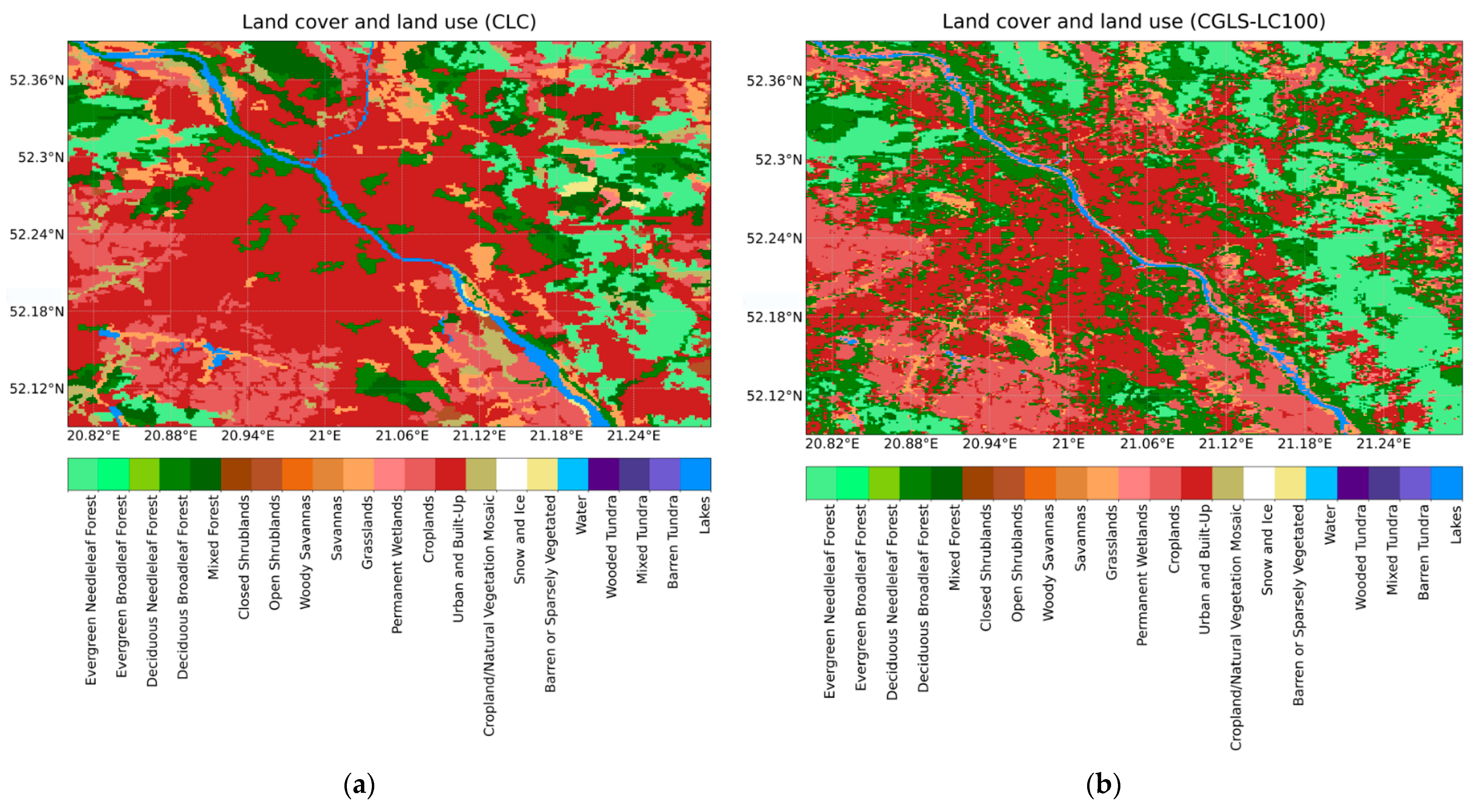
To implement stage three, the reclassified LULC CGLS-LC100 data were transformed into binary data [46]. The data format was changed using GDALL [12]. In the WRF model, the geogrid data concerning LULC are processed in the WRF Processing System (WPS). In the WPS, the geogrid module interpolates the geographic data to the resolution of the computational domains. The nearest neighbor method was used to interpolate the CGLS-LC100 categorical data of LULC classes to the model grids. To initialize the WRF model data calculation with CGLS-LC100, CLC, or default data, it is necessary to declare this at the WPS list. The order of the declaration of the geographical data to be used by the WPS is important because when the area is out of the coverage of the first set of data, the model is using the second one, or if the areas are adjacent, the module completes the missing area with the data from the second set [22]. The process of implementing CLC data into the WRF model was presented in a previous article [22] by the authors. The visualization of the overclassified LULC CLC and CGLS-LC100 classes to MODIS classes is shown in Figure 2. It is worth highlighting that different classification methods were used to compile those LULC data from the satellite data. CLC data are based on manual classification, and CGLS-LC100 data are based on pixel-based (spectral) classification. The thematic classification accuracy of CLC data is above 85%, and CGLS-LC100 is above 80%. The area of Figure 2 includes the area of the city of Warsaw, which was taken as the study area.
For the analyzed synoptic situations, a detailed analysis of the forecast errors at individual measuring stations and aggregate analyses of the errors for individual days were carried out. The values of the average forecast errors for all analyzed synoptic situations and meteorological measuring stations were determined. The data extraction and calculation of the verification indices characterizing the quality of the forecasts were performed in Python language [56].
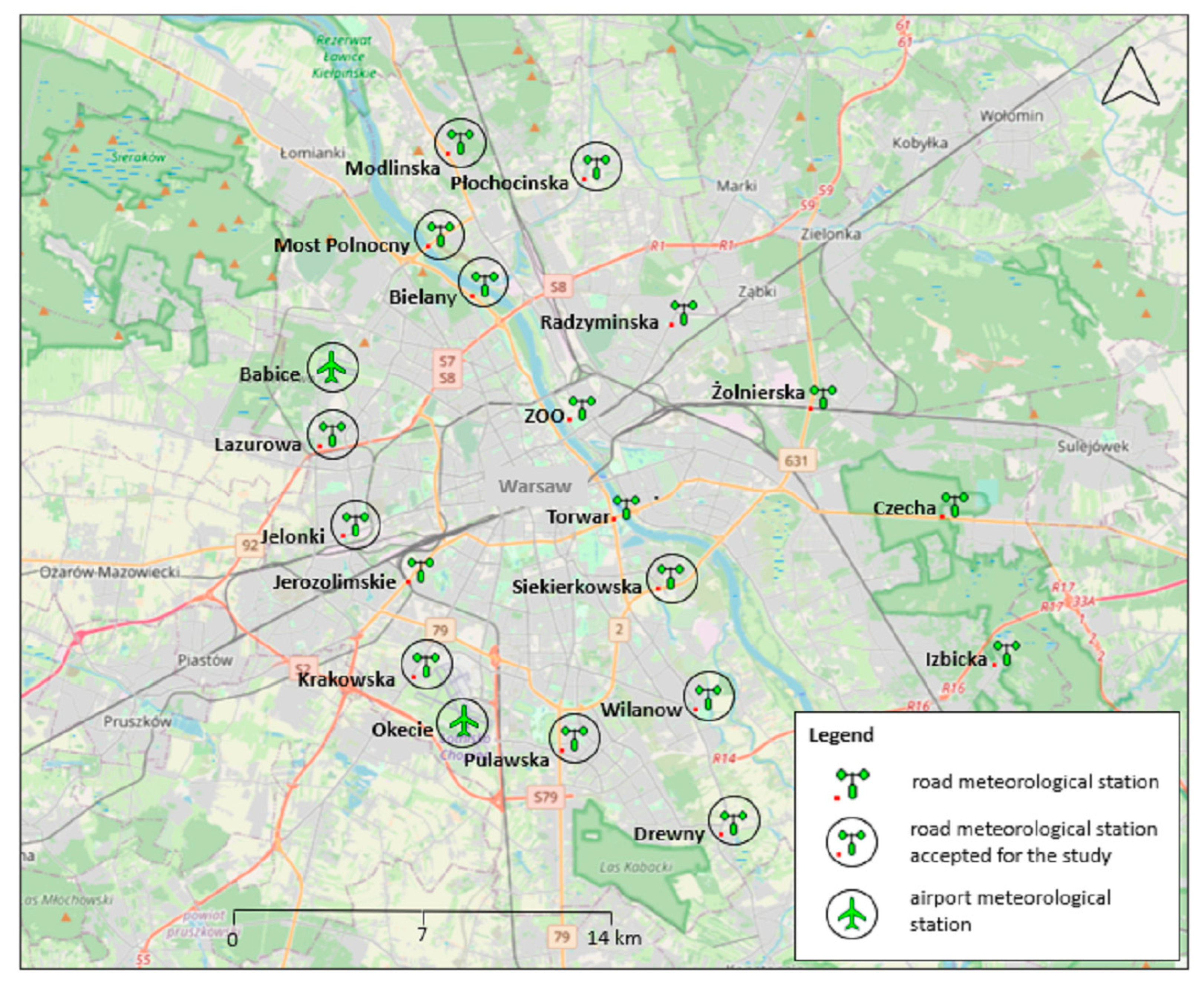
To verify the quantitative meteorological forecasts, the following statistics were calculated: mean error (ME), mean absolute error (MAE), root-mean-square error (RMSE), mean squared error (MSE), bias error (BIAS), Pearson correlation coefficient (R), and normalized root-mean-square error (nRMSE) (Table 2). To verify the results of the numerical modelling of weather forecasts, hourly data from a network of road meteorological stations [49] and airport meteorological stations within Warsaw were used (Figure 3).
Table 2. Definition of the statistical indicators [57,58,59].
IndicatorsDefinition
Mean error (ME)ME =  i = 1 n ( f i o i ) n
Mean absolute error (MAE)MAE =  i = 1 n | f i o i | n
Root-mean-square error (RMSE)RMSE =  i = 1 n ( f i o i ) 2 n
Mean squared error (MSE)MSE =  i = 1 n ( f i o i ) 2 n
Pearson correlation coefficient (R)R =  i = 1 n ( f i f ) ( o i o ) i = 1 n ( f i f ) 2 i 1 n ( o i o ) 2
Bias error (BIAS)BIAS =  1 n i = 1 n f i 1 n i = 1 n o i
Normalized root-mean-square error (nRMSE)nRMSE =  R M S E 100 % 1 n i = 1 n o i
Figure 3. Network of meteorological stations of the City Cleaning Board within the city of Warsaw accepted for the study (in black circles) and airport meteorological stations (based on reference [60]).
Remotesensing 15 02389 g003
The network of road meteorological stations consists of automatic meteorological measurement stations located in the strip of national roads, which allow the forecasting of atmospheric phenomena occurring in the road area, especially the phenomenon of glaze, to support seasonal road maintenance decision-making processes. The number of stations installed in each road section depends strictly on the microclimatic conditions of the road sections by maintaining, as far as practical, standards of representativeness of the meteorological measurements; hence, they characterize local-to-microscale conditions [61,62]. The network of measuring stations in the Warsaw agglomeration consists of eighteen measuring stations, as shown in Table 3. Because not all measuring stations carry out measurements of wind speed and direction, for this study, we used eleven stations, from which measurements of all four analyzed meteorological parameters were available. Other data used to verify the results of numerical modeling of weather forecasts were obtained from airport meteorological stations Okecie (EPWA) with coordinates: 52°9′46″N, 20°57′40″E [49] and Babice (EPBC) with coordinates: 52°16′0″N, 20°55′0″E.

2.2. Study Area and Synoptic Situations

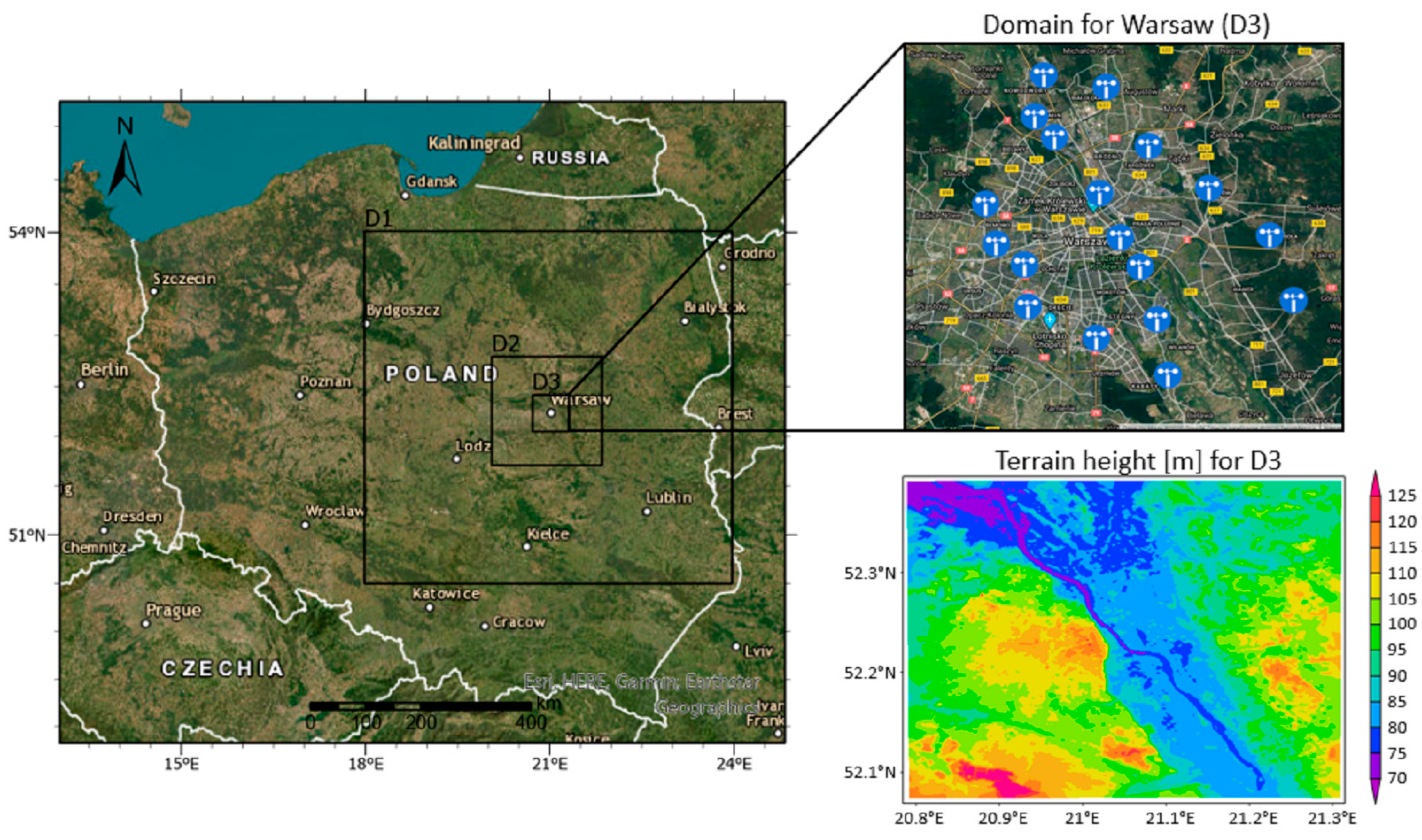
The area of the capital city of Warsaw was taken as the study area. This city is located in the central-eastern part of Poland (Figure 4). Built-up and urbanized area account for almost 60% of the total city’s area. This influences the formation of conditions characteristic for urban weather in Warsaw. Among other things, ten ventilation corridors of the city are observed in the Warsaw area. The impact of anthropogenic factors is important in weather modeling. Urban forecasting requires increasing the computational resolution of the model and, thus, also provides appropriate geographic data that will be used by the model. As for the larger computational domains of the WRF model for Warsaw, their area often includes the non-CLC area as well.
For the area of Poland, CLC data are available, yet, unfortunately, their coverage ends at the eastern border of Poland. This motivated the article’s authors to research the use of alternative sources of high-resolution CGLS-LC100 data, whose coverage also includes the area in the east of Poland.
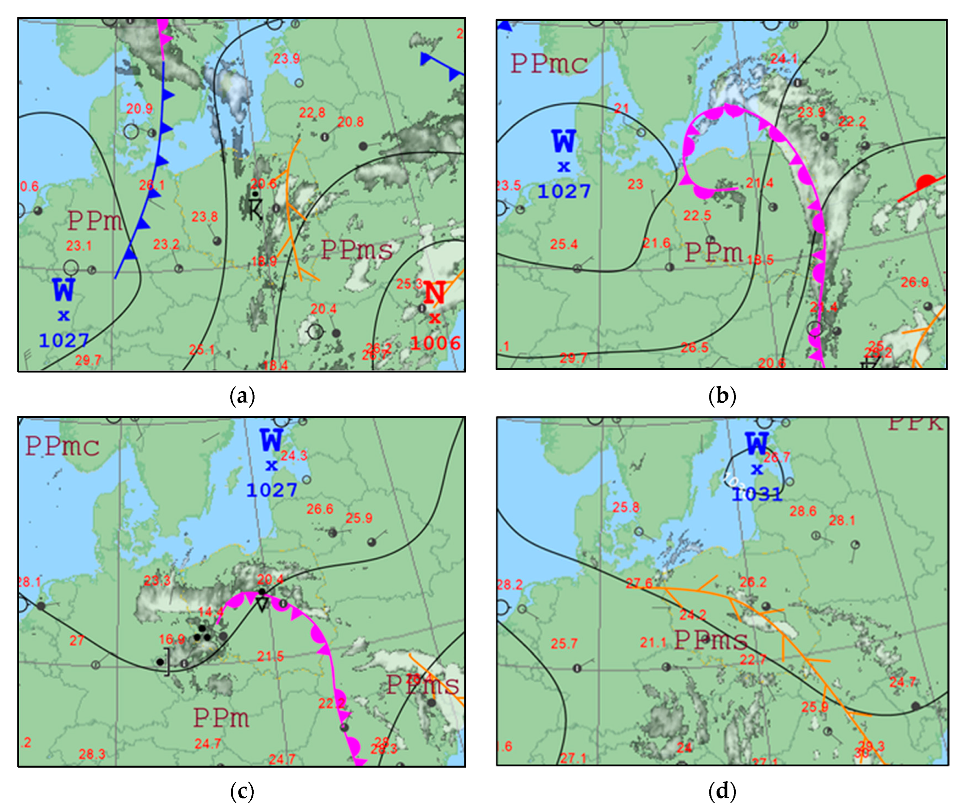
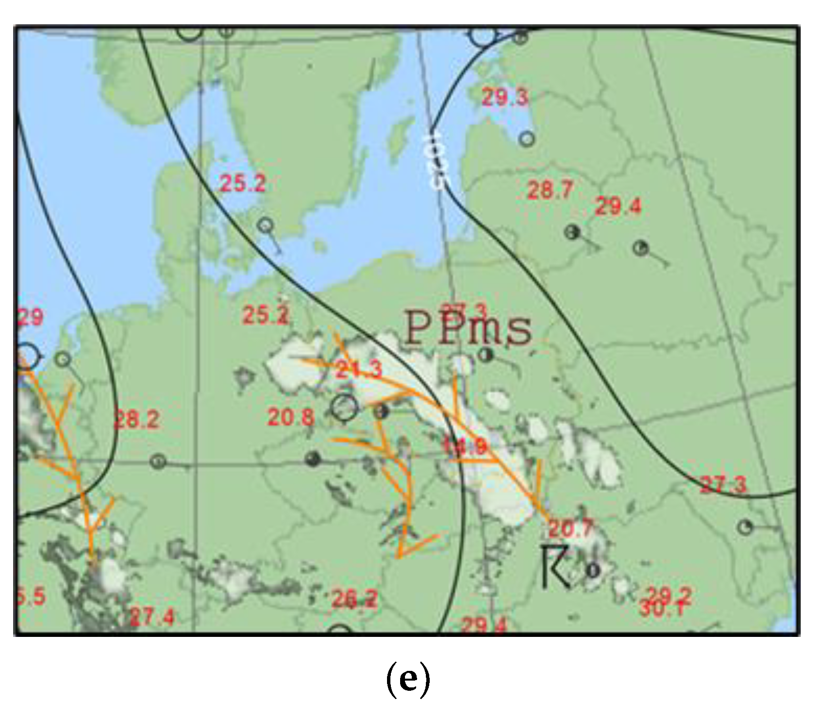
For the analysis, a random period was selected, during which there was eastern advection in Warsaw conditioned by the distribution of baric systems (Figure 5). This was the period from 22 June 2020, 00:00 UTC, to 27 June 2020, 00:00 UTC. During the first part of the term (22–24 June 2020), the weather in Warsaw was shaped between the eastern part of the anticyclone over France and the bordering rear part of the cyclone over the Black Sea. The occurring unstable air mass, additionally aided by convergent airflow, favored the formation of a convergence line (22 June 2020). During the day, Cu and Cb clouds were present over Warsaw.
In the following days (23–24 June 2020), the formation of a cold front of an occluding system could be observed, along which thunderstorms commonly occur in summer. In the filling gulfs and away from the center of the low, the cloud systems of the occluded fronts have less vertical extension and are strongly stratified. It is worth noting that this front was associated with an upper low whose center moved from the Baltic Sea over western Poland to the Czech Republic.
In the second part of the analyzed period (25–27 June 2022), the high-pressure center from Western Europe moved over the northern Baltic Sea and farther through the Baltic countries to western Russia. During this period, Warsaw was under the influence of the western edge of the mentioned anticyclone. In summer, at the western edge of the anticyclone with high temperature, humidity, and thermodynamic instability, storms often occur in the formation of convergence lines. Furthermore, in diffuse pressure fields and on the western edges of inactive anticyclones, when the air mass in the ground layer heats up, and the humidity of this mass increases, with significant air mass instability, when there are conditions for strong daytime heating of the ground air layer, and high humidity persisting at an altitude of several kilometers and the absence of inversion and isothermal layers, thunderstorms form in homogeneous air masses.
With reference to the previously mentioned eastern inflow over the Warsaw area, it is worth noting that from the practical use of numerical weather forecast models by the synoptics, it appears that with eastern inflows over the Polish area, the models are characterized by lower forecasting capabilities than with western inflows, which may be caused, among other reasons, by a smaller number of observations and radiosonde data from Eastern Europe. It is worth noting that the formation of convergence lines is the most surprising weather pattern and is generally not well forecasted. In general, convergence lines are not always predicted in numerical weather forecast models, especially those with low spatial resolutions. The local factors that favor convergence lines (landforms, local pressure differences, small changes in atmospheric conditions at different altitudes and sea breezes) are difficult to account for in numerical models, leading to imperfections in their forecasting. Forecasting convergence lines requires synopticians to keep a close eye on the development of atmospheric processes to be able to warn the concerned institutions in time about the possibility of their occurrence because if there are thunderstorms on the convergence line, then it is called a squall line.
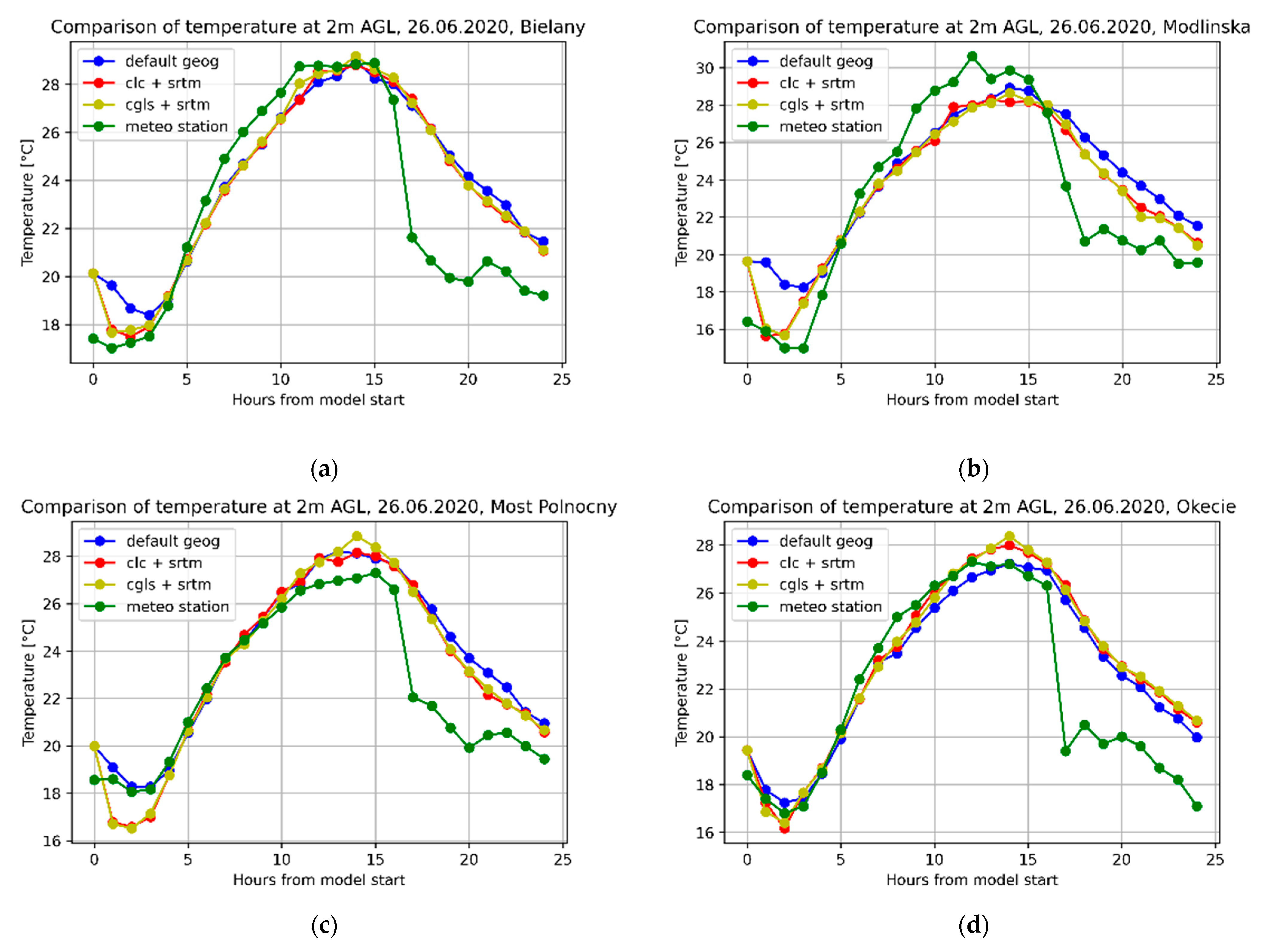
It is interesting to note that on 26 June 2020 (Figure 5 and Figure 6), there was a line of convergence over Warsaw, which was not forecasted by the WRF model. Therefore, the model results deviated significantly from the actual conditions. According to the model, the daytime temperature was expected to have a normal diurnal distribution, and the observational data show that there was a pronounced drop in temperature after the convergence line passed. Squall lines are narrow zones with thunderstorms, precipitation, and squalls with characteristics like those of cold fronts, but which are local and short-lived results of thunderstorm activity. They often form in the warm and unstable sectors of low-pressure systems before cold fronts or on the edge of high-pressure systems where incoming cold air pushes warmer air upwards, causing convective phenomena to develop. In other words, the term describes an unstable air mass characterized by increased turbulence and the development of convection with corresponding cloudiness.

2.3. WRF Model

The WRF model is a non-hydrostatic mesoscale weather forecast model. The model has been designed and developed continuously for more than 22 years, among others, by the National Oceanic and Atmospheric Administration (NOAA), National Centers for Environmental Prediction (NCEP), National Center for Atmospheric Research (NCAR), Air Force Weather Agency (AFWA), Forecast Systems Laboratory (FSL), Federal Aviation Administration (FAA), and the United States Air Forces (USAF) [8]. The WRF model output accuracy depends on the accuracy of the input data, the topography of the terrain, geographical data, the quality of the parametrization of the physical processes it models, the model version, and synoptic situations. For the purposes of this study, WRF model version 4.2.1 was used. The WRF model set-up for the conducted studies is presented in Table 4. The WRF model was run on the data (first approximation fields and boundary conditions) of the superior Global Forecast System (GFS) model with a resolution of 0.25° (~28 km) [64]. Due to the higher spatial resolution of the regional and mesoscale WRF simulations compared to the GFS, downscaling was carried out using multiple nesting.
It is worth noting that the spatial resolution of the global model is sufficient to provide data for regional, mesoscale, and even microscale models. For comparison, synoptic stations in Poland are spaced approximately every 50 km. The spatial resolution of the model used for the simulation was 2.5 km for the first domain (D1), 500 m for the second (D2), and 100 m for the third (D3). The forecasts for each day started at 00:00 UTC, the spin-up time was 6 h, and the forecast time was 24 h with one-hour output data. The selection of parametrization schemes of the WRF physical processes was conducted based on the studies for the Central European area [64,65] and other recent studies related to this subject [66,67]. Based on that, the revised MM5 Monin–Obukhov surface layer scheme [9,65,66,68] was used in this study (for all domains). For planetary boundary layer (PBL) parameterization, the Yonsei University Scheme (YSU) [9,64,65,69] was applied for the first domain. In the second and third domain, explicit vertical diffusion was used directly (non-PBL parameterization) [9,65,70,71,72]. For those domains, the horizontal and vertical eddy viscosities were determined using 3D Smagorinsky turbulence [9]. For all domains, microphysics parametrization WSM6 [7] and RRTMG longwave and shortwave radiation schemes [8] were used.

3. Results

As a result of simulating the WRF model in three variants, the distributions of basic meteorological parameters (temperature (Figure 6), relative humidity, wind direction and speed) were obtained.
The results were compared with the observations and then, to determine the quality of the forecasts of the meteorological parameters, they were verified based on the values of statistical indicators (Table 2).
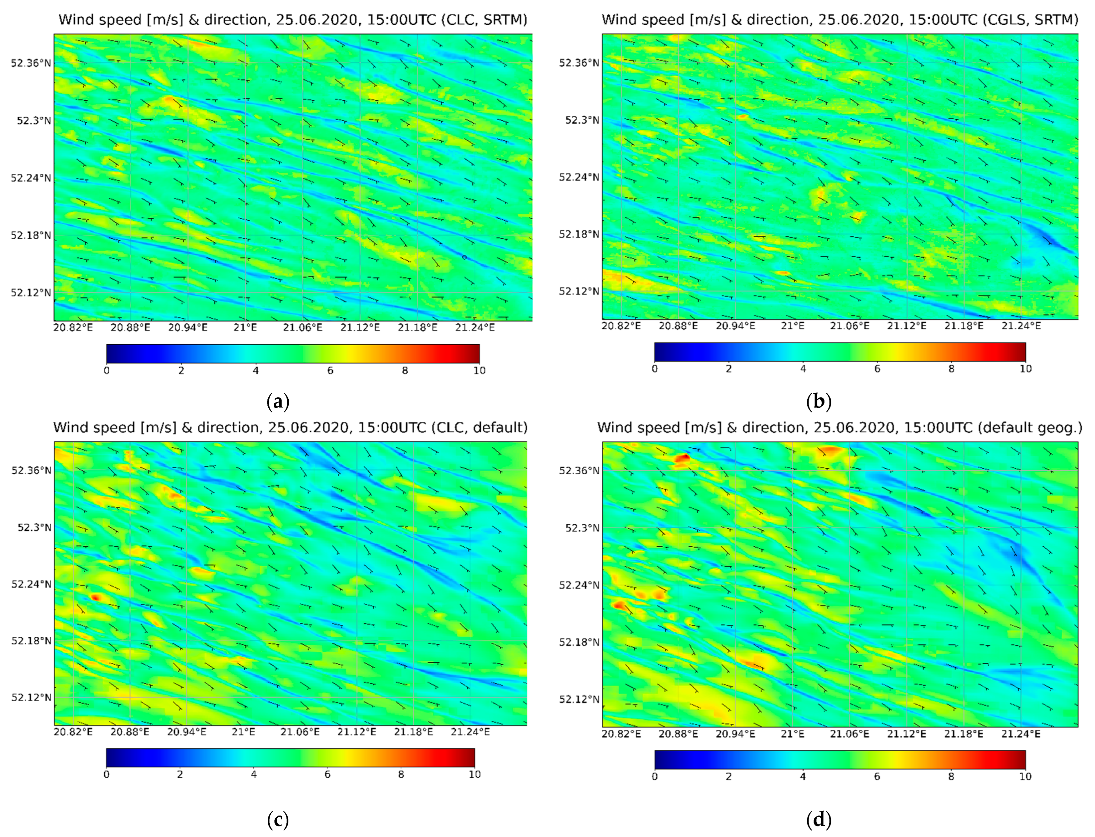
To show that not only the terrain but also land cover influence the wind simulation, the example results of different geographical data setups for the third domains are summarized in Figure 7. The forecast of wind speed and direction is influenced, as are the forecasts of the other elements analyzed, by both the topography of the terrain and its cover. Land cover roughness and heat capacity significantly influence wind formation, distribution, and intensity.
The analysis of the forecast error values of individual parameters was divided into the analysis of forecast errors for individual days for all analyzed stations and the analysis of errors at a given measuring station for the complete study period. The value of the forecasting errors of individual parameters averaged over stations and days was also calculated (Table 5 and Table 6). Analyses of the values of the temperature forecast errors for individual days average over stations (Figure 8) showed that in 80% of the situations studied, the use of CLC or CGLS-LC100 data improved the obtained results. This improvement was greater for simulations using CLC data than those using CGLS-LC100.
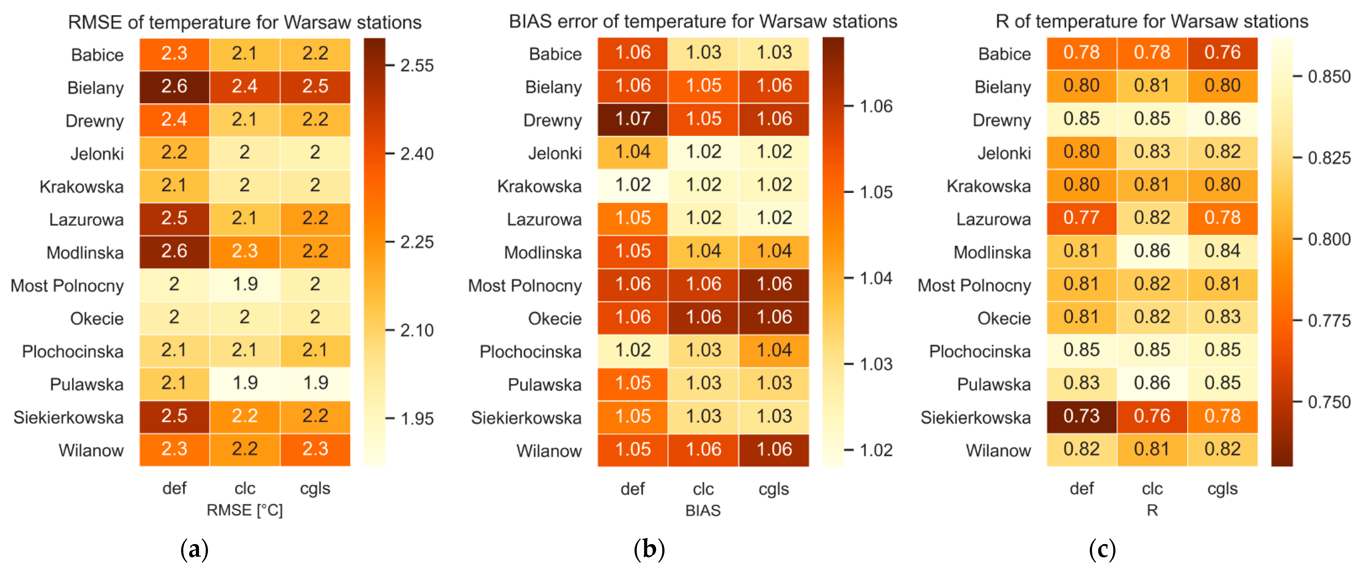
Analysis of the RMSE values for the individual measurement stations (Figure 9) averaged over days showed the greatest improvement in temperature forecast results when using CLC data (the matrix mesh near ideal value has lighter color). The improvement over the simulation in the default configuration also occurred when CGLS-LC100 data were used. The analysis of BIAS values for individual measuring stations showed that in only at two stations (Plochocinska and Wilanow) of the thirteen analyzed stations, the value for the default simulation was better than for the CLC or CGLS-LC100 simulations. The value of the Pearson correlation coefficient (R) of temperature forecast, an average over stations and days, was the best for the simulation on CLC data, and it was 0.82 (Table 4).
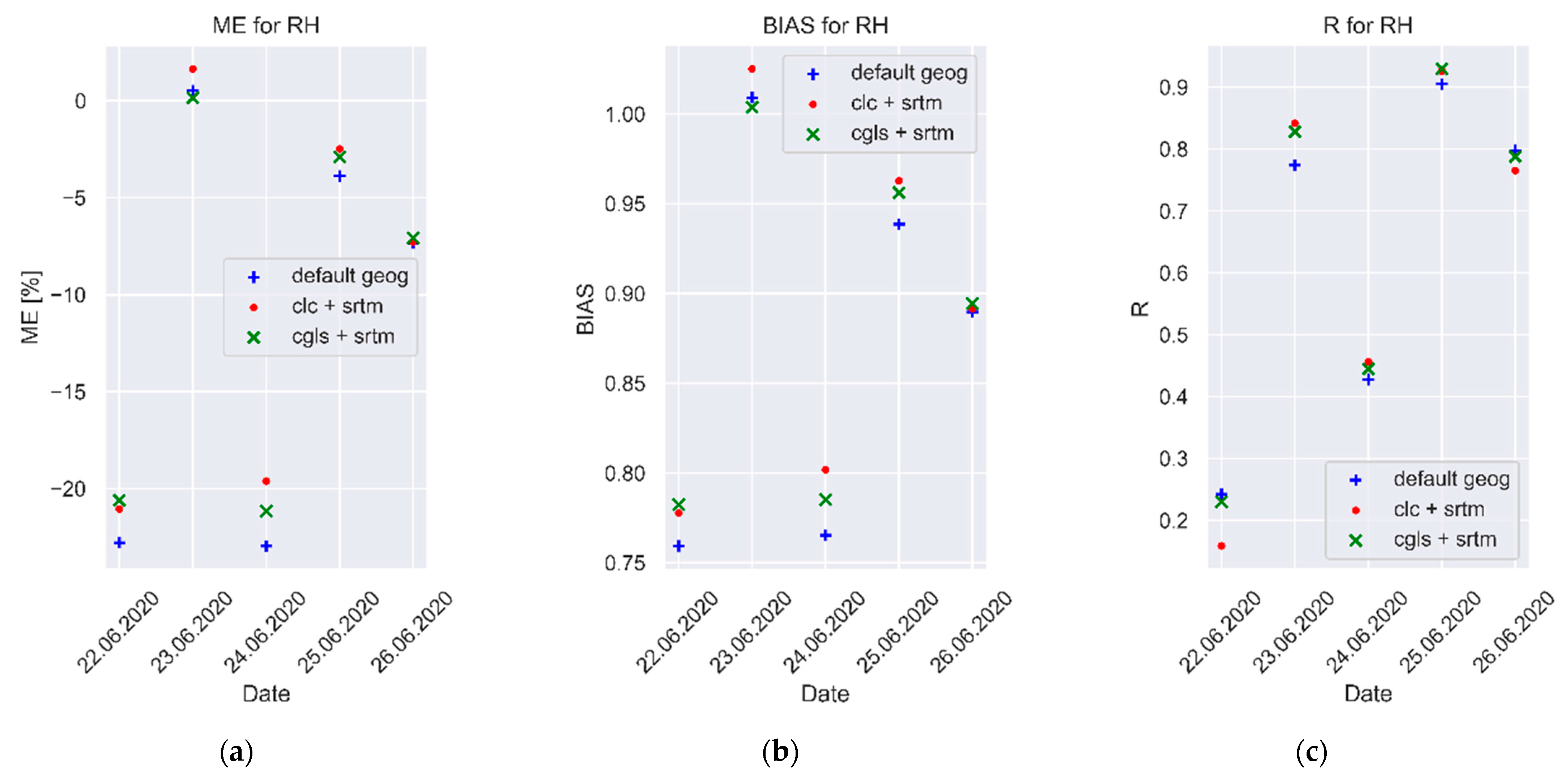
The verification of the relative humidity forecasts for the synoptic situations analyzed revealed (Table 6, Figure 10) that the near-ideal value of forecasts, as determined by Pearson’s correlation coefficient (R), was obtained by the model simulations using CLC. BIAS indicated higher agreement between forecasts and observations for CLC simulations. Moreover, ME, MAE, RMSE, and MSE showed the highest agreement with observations for the simulations plotted using CLC. For 80% of the analyzed cases, the use of CLC or CGLS-LC100 data effectively improved relative humidity forecasts.
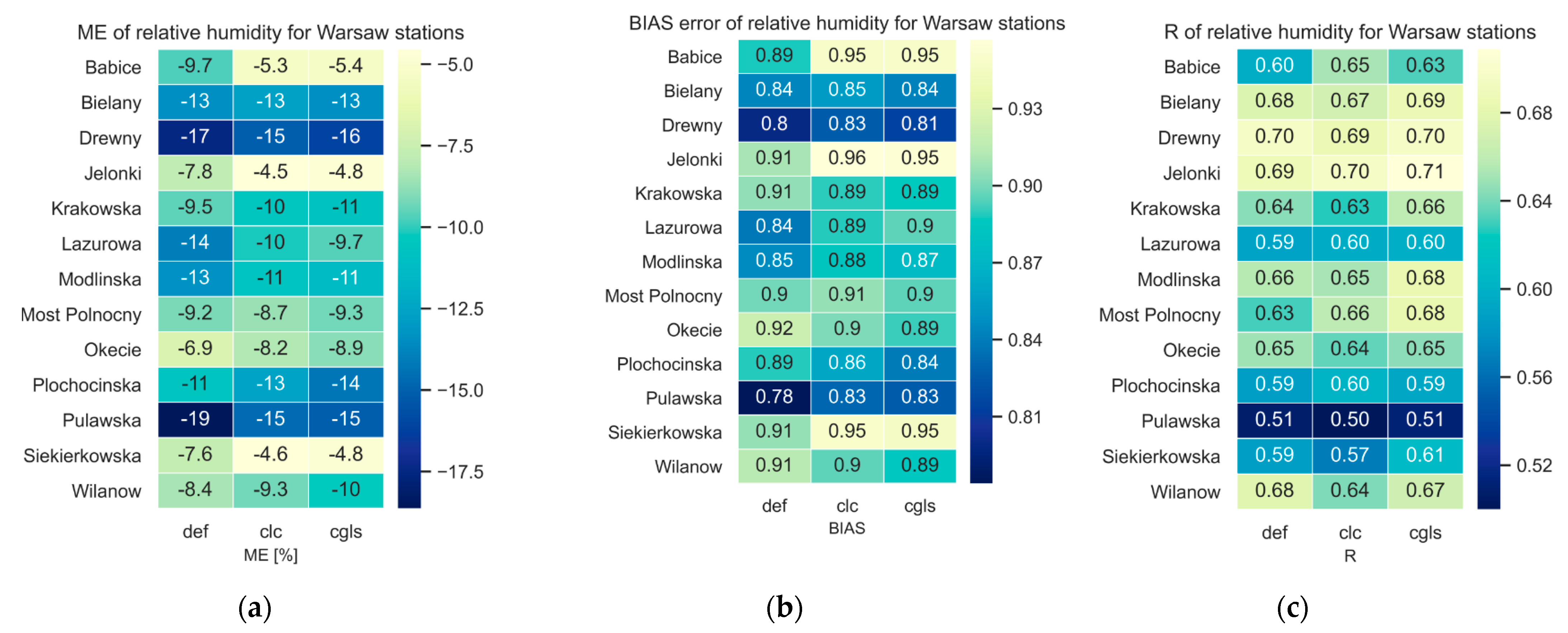
The verification of the relative humidity forecasts at individual gauging stations (Figure 11) showed that at 69% of stations, the use of CLC or CGLS-LC100 data improved the obtained weather forecast results compared to simulations using default geographical data. Despite the fact that the average value (for all surveyed stations and for the whole analyzed five-day period of the simulation) of the RMSE for relative humidity forecast was better (the lowest) for simulations using CLC when analyzing the average value of the correlation coefficient (R), the best result was achieved for simulations on CGLS-LC100 data, and it was 0.64 (Table 6).
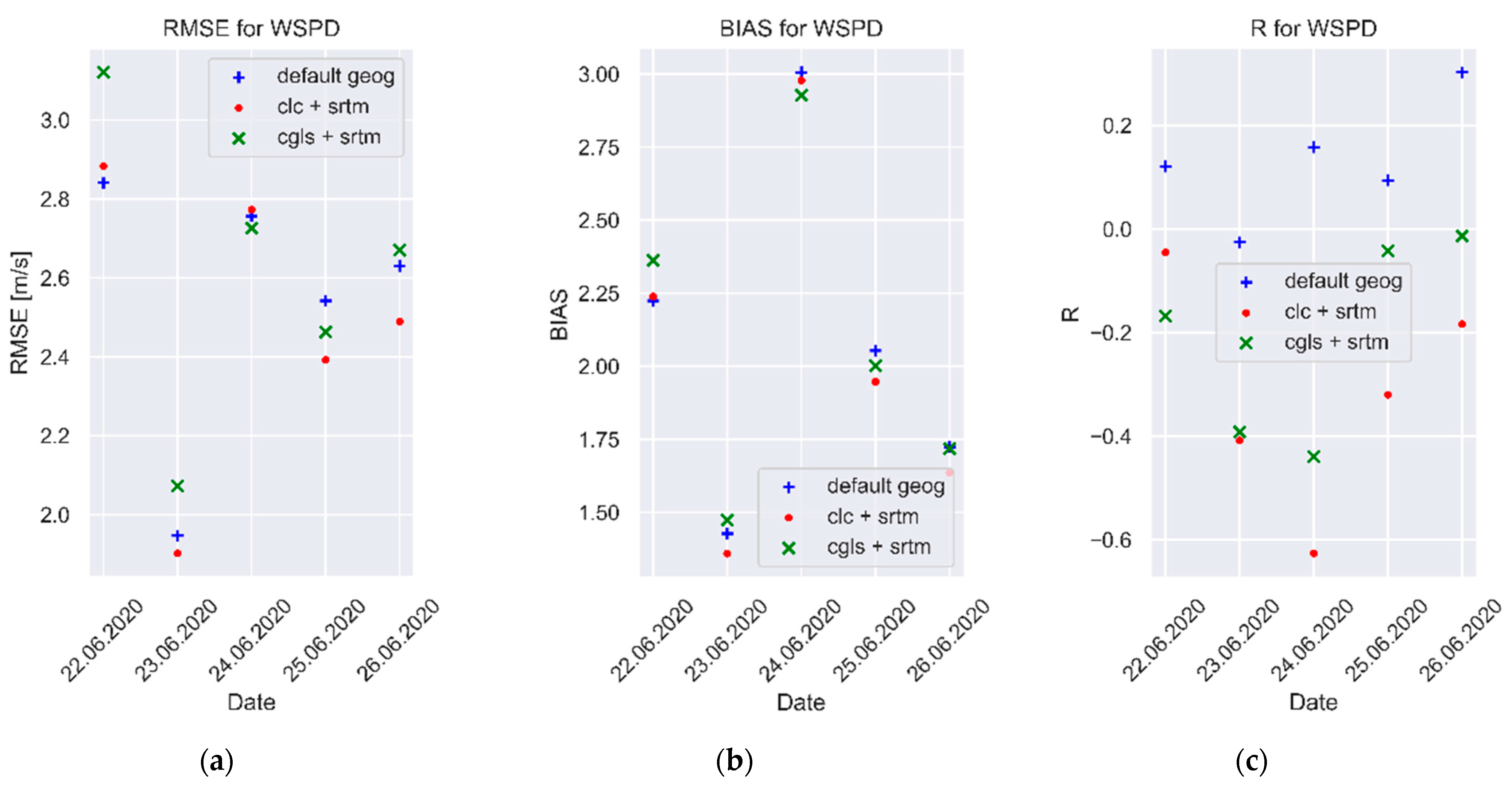
The verification of the wind speed forecasts for the examined synoptic situations in the three different variants showed that the values of the mean errors (ME, MAE, MSE, and RMSE) were the lowest for the simulation using the CLC data (Figure 12). BIAS also showed the highest compliance for CLC simulations (Table 6). For 60% of the analyzed cases, the use of CLC data enhances the capability of receiving more accurate wind speed forecasts.
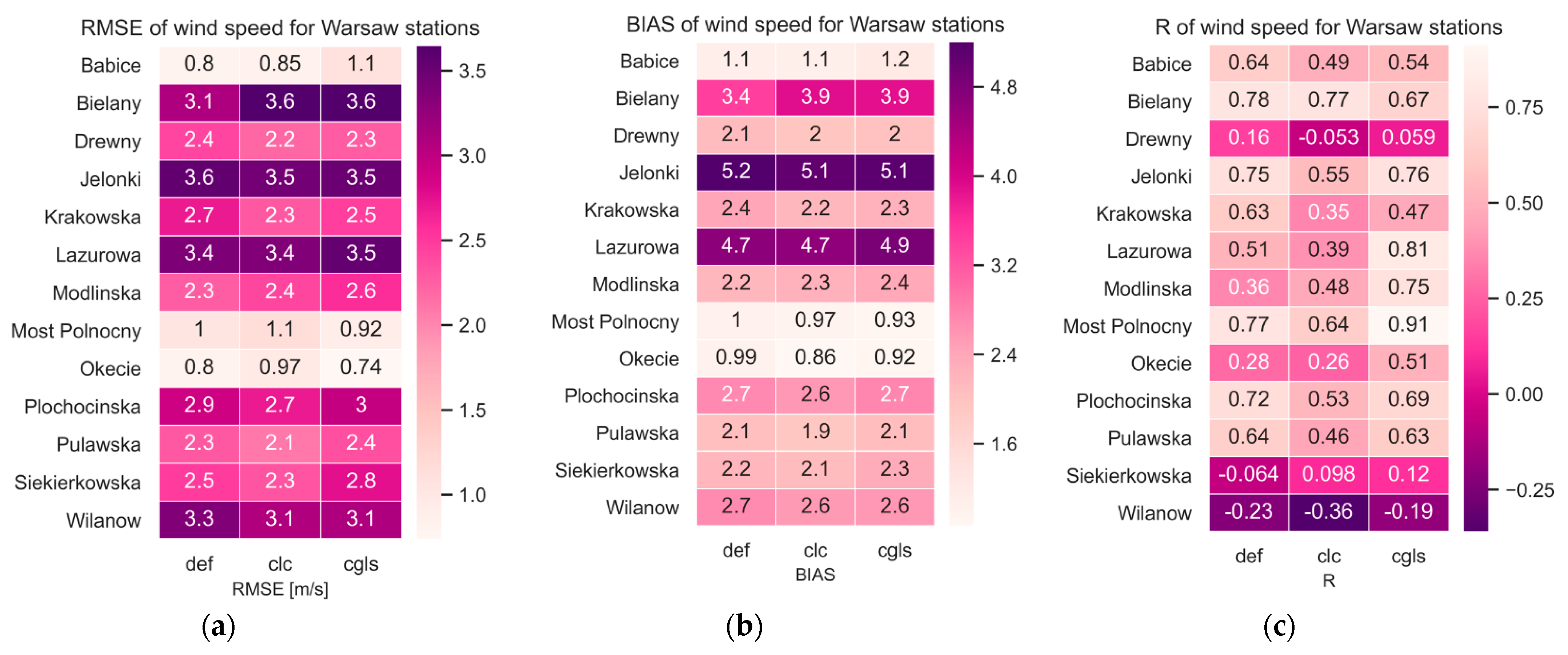
A detailed analysis of the errors at individual stations showed that for 54% of the stations studied, the BIAS value for CLC and CGLS-LC100 simulations was closer to the ideal value than for simulations of the default parameters (Figure 13). The value of the Pearson correlation coefficient (R) of the wind speed forecast was the best for the simulation on CGLS-LC100 data, and it was 0.52 (Table 6).
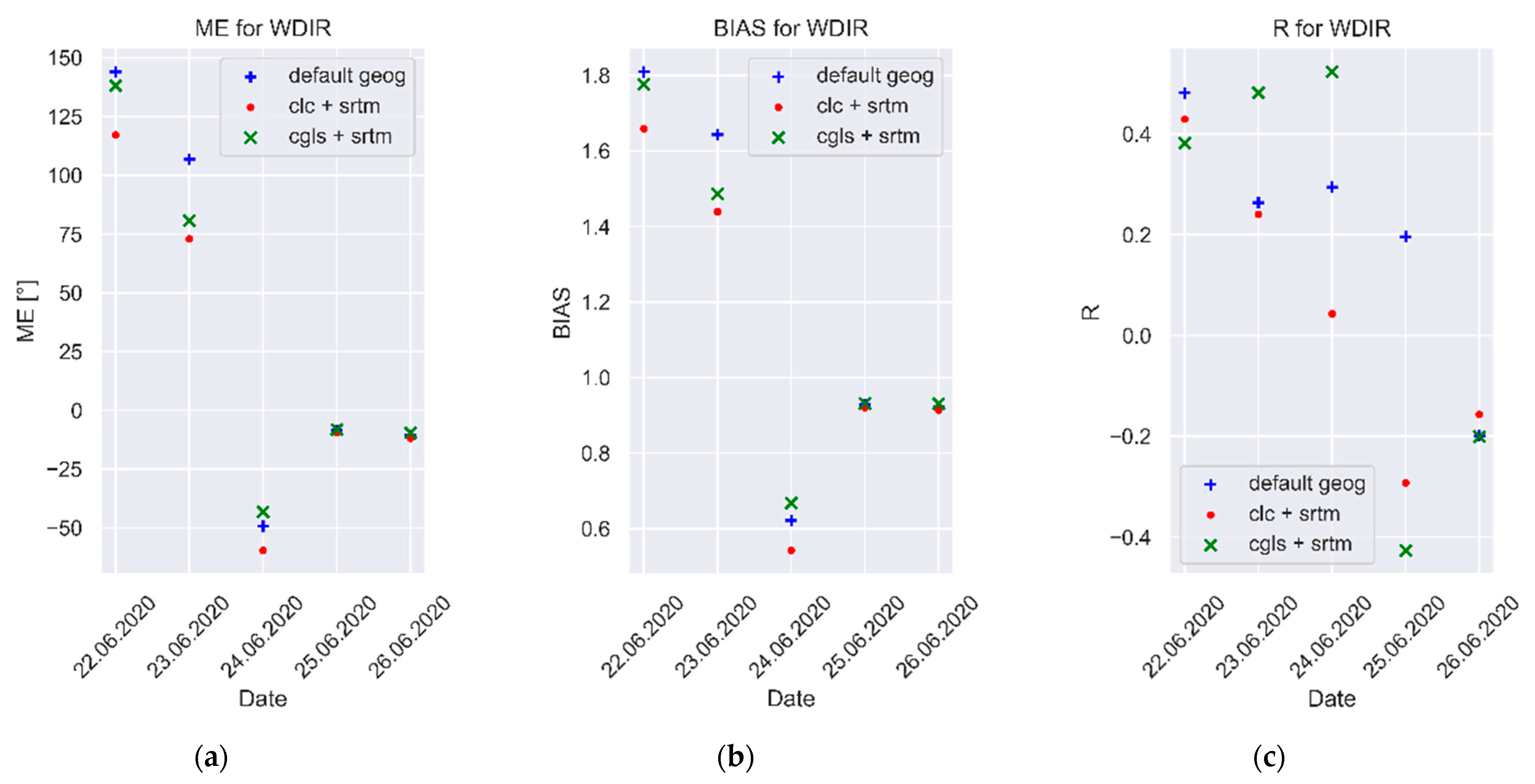
Analysis of wind direction forecasts for the examined synoptic situations showed that the value of mean error (ME), mean square error (MSE), and BIAS reached the most desirable value for simulations using CLC (Table 5 and Table 6, Figure 14). Furthermore, simulations using CGLS-LC100 showed higher accuracy in terms of wind direction forecasts than simulations on default data.
A detailed analysis of the errors at individual stations showed that for 77% of the stations studied, the BIAS value for CLC and CGLS-LC100 simulations was closer to the ideal value than for simulations on default parameters (Figure 15). The value of the Pearson correlation coefficient (R) of the wind speed forecast was the best for the simulation on CGLS-LC100 data, and it was 0.25 (Table 6). RMSE and R were more sensitive to large forecast errors, so the errors shown for several stations outweighed the final result of the statistical analyses for all weather stations (Figure 15).
Table 5 and Table 6 show the average forecast errors of forecast parameters for the whole analyzed period and all of the analyzed meteorological stations (road network and airport stations). The average forecast error in this study is described as the error average for stations and days. Table 7 and Table 8 present the verification results (average for stations and days) exclusively for airport meteorological stations, which meet the WMO requirements for location and, thus, should yield more objective analysis results.
For temperature and relative humidity forecasts for both the airport weather stations and all of the analyzed weather stations, the smallest average forecast errors (RMSE, ME, MAE, and MSE) were obtained by the CLC simulations. The errors in the CGLS-LC100 simulations were slightly higher. Simulations using default data introduced the worst results. Furthermore, the BIAS and R-factor values showed the highest accuracy in terms of temperature and relative humidity forecasts for simulations for airport stations and temperature forecasts for simulations for all of the analyzed weather stations using CLC (Table 6 and Table 8). The average value of the temperature forecast improvement for simulations using CLC data compared to the default data was 0.19 °C. The average value of the difference between the observed and modeled temperatures was 0.79 °C in the CLC simulation, 0.85 °C in the CGLS-LC100 simulation, and 0.98 °C in the simulation using the default data (Table 5). According to ICAO annex 3, the temperature for aviation purposes should be predicted with an accuracy of ±1 °C. Therefore, even such a seemingly small improvement in model forecast capability is important for synoptics. The statistical verification of the predicted parameters showed (Table 6) that for the 2 m temperature prediction, the use of CLC data allowed the nRMSE to be decreased by 0.81% and by 0.67% when using CGLS-LC100 data compared to the results obtained in default geographical data simulations.
The greatest improvement in the average relative humidity forecast value was recorded for the CLC simulation. For the three simulation variants analyzed, the average relative humidity forecast error for the CLC simulations compared to the default simulations decreased by 1.54% (Table 5). For relative humidity forecasts, the decrease in nRMSE for the simulations using CLC was 1.47% and 1.29% for CGLS-LC100 compared to the default simulations (Table 6). The value of the average difference between the observed and modeled relative humidity was −9.75% for the CLC simulation, −10.31% for the CGLS-LC100 data, and −11.29% for the default data (Table 5). It is notable that for the analyzed period, the model overestimated the average value of the forecast temperature by about 0.8 °C to 1.1 °C (Table 5 and Table 7). As for relative humidity, it underestimated its value by 6.8% to 11.3% (Table 6 and Table 8). These significant errors may have been caused by the presence of squall lines during the analyzed period, which are not always properly forecasted by the WRF model (Figure 6).
As far as the wind speed analyses for airport stations and all of the analyzed meteorological stations are concerned, the lowest value of the mean forecast error (ME) was obtained by the CLC simulation, a slightly higher error was obtained by the simulation using default data, and the worst result was noted for the simulation using CGLS-LC100 (Table 5 and Table 7). An increase of 2.90% in nRMSE was recorded for the wind speed simulation using CGLS-LC100 data compared to the simulation using default data (Table 6 and Table 8). The value of the improvement in wind speed forecasts was below the acceptable wind speed measurement error (0.5 m/s). According to ICAO annex 3, the wind speed reading required for aviation should be predicted with an accuracy of ±2.5 m/s and a wind direction of ±20°. The average value of the difference in wind speed measured to result from the model was 2.15 m/s for the simulation on the default data, 2.01 m/s for the CLC simulation, and 2.19 m/s for the CGLS-LC100 simulation. The mean value of the improvement after applying the CLC data was 0.14 m/s (Table 5 and Table 6). It is also worth noting that in the case of the wind speed forecast, the value of the average forecast error (for stations and days) was about 2 m/s higher for stations from the network of road meteorological stations (Table 5 and Table 7) in comparison with the values obtained for airport meteorological stations (or stations situated in open areas, such as Most Polnocny). This may be caused by the failure to maintain a 30 m separation of the measuring station from terrain obstacles.
As for the wind direction analysis for all analyzed meteorological stations, the lowest mean forecast error (for stations and days) was obtained for simulations with CLC. Moreover, for the simulations created with CGLS-LC100, lower values of the mean error of the wind direction forecast were obtained than for the simulations on the default data.
For wind direction, a decrease in nRMSE of 5.55% was recorded for the simulation using CLC and a decrease of 4.53% for the CGLS-LC100 simulation compared to the simulation using default data (Table 8). The average difference (for all stations and days) between the wind direction calculated by the model and measured was 36.46° for the default simulations, 21.79° for the CLC simulation, and 31.52° for the CGLS-LC100 simulation (Table 5). The use of CLC simulations resulted in an average improvement of 14.68°.

4. Discussion

The correctness of forecasting atmospheric phenomena is determined by the accuracy of the basic meteorological parameters forecast by the numerical model; therefore, it is important to improve the accuracy of forecasting basic meteorological parameters even slightly, for example, by updating the geographical data (LULC, topography) used by numerical weather prediction models. Measurements, as well as the prognostic values of meteorological parameters in numerical weather prediction models, are used to develop forecasts of atmospheric phenomena (e.g., glaze or fog) or prognoses of the amount of energy obtained from renewable sources. WMO requirements [50] for the accuracy of measurements of individual meteorological parameters indicate the need to provide highly accurate measurements of individual meteorological parameters for both aviation and synoptic meteorology. Based on that, the accuracy of the meteorological measurements used for synoptic, aviation, or agrometeorological purposes should be as follows: temperature, ±0.1 °C; relative humidity, ±1%; wind speed, ±0.5 m/s; and wind direction, ±5°. According to this article’s authors, those values could be equated with the accuracy requirements of an ideal weather forecast model. According to the received values of forecast errors, it could be seen that the received values of the prognosed parameters meet the ICAO requirements for an operationally desirable accuracy of forecasts, which should be as follows: temperature, ±1.0 °C; wind speed, ±2.5 m/s; and wind direction, ±20°, for at least 80% of cases.
Based on conducted studies, it can be seen that the implementation of higher-resolution geographical data has allowed for increased forecast accuracy for Warsaw. The implementation of higher-resolution and more up-to-date LULC data resulted in receiving more consistent values in terms of temperature and relative humidity forecasts. The greatest improvement was received in terms of CLC data implementation. For CGLS-LC100 data implementation, improvements also occurred compared to the default simulations. The results obtained after the implementation of the CLC data did not confirm the temperature overestimation effect observed in Northern Italy [31], but confirmed the results received after global LULC data implementation for Xinjang in northwest China [13]. The improvement in temperature forecast after CLC data implementation to the WRF model was also confirmed for Berlin [38] and Austrian regions [39]. The use of USGS data as a default for studies concluded that for Berlin, the temperature is underestimated [38], whereas for the use of MODIS data as a default, there was overestimation in temperature for Warsaw. In addition, for the analyzed period and the stations studied, the forecasted temperature value after the implementation of the high-resolution LULC data showed a decrease, which is caused by a better representation of small green areas in the city.
For wind speed forecasts after higher-resolution geographical data implementation for the analyzed areas, a reduction in wind speed was visible. The wind speed decrease was not as high as noted for other regions in Europe [36], which could be caused not only by the roughness length of land use and land cover classes, but also by the better representation of friction in higher-resolution topography. The received differences in wind speed forecasts between airport and road meteorological network stations indicate that there are microscale environmental influences in the urban area in terms of the measurement of wind speed and direction by the road meteorological stations. The BIAS and RMSE values illustrated that the simulated near-surface parameters improved when using the highest and more-updated land use and land cover data with a topography adequate to its resolution. The received results indicate that for the analyzed area, a better representation of LULC data is achieved through CLC data than CGLS-LC100, which confirmed its higher thematic accuracy.
Overestimation of the wind speed forecasts at the WRF model during spring and summer was also emphasized in other works [73]. Some steps for an additional increase of wind speed forecast verifiability can be taken; for example, the use of additional measurements of wind speed in the planetary boundary layer from the Doppler wind LiDARs (Light Detection and Ranging) [74] can provide high-accuracy reference data to validate the NWP model. Moreover, that data assimilation can improve the WRF accuracy of wind simulations [73,75].
Our research shows the possible effect of basic meteorological parameter forecast improvement when using more accurate LULC data in very high-resolution WRF modeling. It is worth emphasizing that the WRF model results can have different accuracy for different seasons, synoptic situations, and localizations. Therefore, to provide a more convincing statistical assessment, the study will be continued considering different synoptic situations over a longer period for different seasons and locations. Moreover, due to the development of increasingly up-to-date land cover and land use data, e.g., from the Sentinel-2 mission [76], research into their impact on numerical weather modeling results will be carried out. The currently available 10 m spatial resolution of land cover and land use data from Sentinel 2 Global Land Cover (S2GLC) provide several opportunities for microscale urban weather modeling.

5. Conclusions

Research studies on the impact of land use and land cover on the results of WRF numerical weather prediction model simulations show that providing more up-to-date LULC data with a higher level of detail can effectively improve numerical weather forecasting of basic meteorological parameters. Most of the studies known to the authors on this topic for the European area have investigated the effect of CLC data implementation on WRF simulation results. Due to the limited coverage of CLC data, the authors developed and tested global land use and coverage data from CGLS at the WRF model. The authors analyzed the impact of implementing high-resolution (100 × 100 m) data on land cover and land use from two independent sources, which are CLC and CGLS-LC100.
For the analyzed period, the use of CLC data allowed for an average improvement in the forecasting of temperature by 0.2 °C, relative humidity by 1.5%, wind speed by 0.1 m/s, and wind direction by 14.7° over the default data. The use of CGLS-LC100 data allowed for an average improvement of 0.1 °C in temperature forecast, 1.0% in relative humidity, 0.04 m/s in wind speed, and 4.9° in wind direction compared to the results obtained on the default data. The results indicate the possible effects of basic meteorological parameter forecast improvement when using higher-accuracy LULC data in high-resolution WRF modeling. Nevertheless, forecasts of meteorological parameters are affected in general by different synoptic situations at each season. Therefore, to ensure the statistical significance of the results, long time series are needed to verify of the new LULC datasets in various synoptic conditions for various seasons and localizations to determine whether CLC and CGLS-LC100 can successfully improve numerical weather forecasts.
Based on the results, it is expected that the use of CLC data more effectively improves numerical weather forecasting capability for Warsaw than CGLS-LC100 data, and, hence, the authors suggest that for high-resolution simulations of the WRF model, if CLC data are available for the area under analysis, these data should be considered to be used first, and in the cases where the analyzed area is outside the range of the CLC, data from the CGLS-LC100 from Copernicus should be used.

Author Contributions

All authors contributed to conducting this research. Conceptualization, methodology, validation, formal analysis, investigation, resources, data curation, J.S.; software, J.S., K.K.; supervision, K.K.; writing—original draft preparation, J.S.; writing—review and editing, K.K.; visualization, J.S. All authors have read and agreed to the published version of the manuscript.

Funding

This research was funded by the Military University of Technology in Warsaw, Faculty of Civil Engineering and Geodesy, Institute of Geospatial Engineering and Geodesy, Statutory Research Funds No. UGB/22-816/2023/WAT.

Institutional Review Board Statement

Not applicable.

Informed Consent Statement

Not applicable.

Data Availability Statement

The data that support the findings of this study are available on request from the corresponding author.

Acknowledgments

The Institute of Meteorology and Water Management—National Research Institute, the NOAA National Weather Service, the National Centers for Environmental Prediction, as well as TRAX elektronik and the Warsaw City Cleaning Authority, which were the sources of the meteorological data used to prepare this paper.

Conflicts of Interest

References

  1. Oke, T.R. The Energetic Basis of the Urban Heat Island. Q. J. R. Meteorol. Soc. 1982, 108, 1–24. [Google Scholar] [CrossRef]
  2. Rozbicki, T.; Kleniewska, M.; Rozbicka, K.; Majewski, G.; Gołaszewski, D. Relating Urban Development and Densification to Temporary Changes in the Air Temperature in Warsaw (Poland). Theor. Appl. Clim. Climatol. 2020, 143, 513–523. [Google Scholar] [CrossRef]
  3. Magdalena, K.; Krzysztof, B.; Paweł, M.; Jakub, S. Urban Climate Research in Warsaw: The Results of Microclimatic Network Measurements. Geogr. Pol. 2014, 87, 491–504. [Google Scholar] [CrossRef]
  4. Lorenc, H.; Mazur, A. Współczesne Problemy Klimatu Warszawy (Contemporary Problems of Warsaw Climate); IMGW: Warszawa, Poland, 2003; ISBN 83-88897-10-1. [Google Scholar]
  5. Lewińska, J. Klimat Miasta: Zasoby, Zagrożenia, Kształtowanie (City Climate: Resources, Threats, Formation); IGPK: Kraków, Poland, 2000; ISBN 8386847956. [Google Scholar]
  6. Budhiraja, B.; Pathak, P.A.; Acharya, D. Studying Surface and Canopy Layer Urban Heat Island at Micro-Scale Using Multi-Sensor Data in Geographic Information Systems. Int. J. Appl. Geospat. Res. 2018, 9, 36–56. [Google Scholar] [CrossRef]
  7. Rath, S.S.; Panda, J.; Sarkar, A. Distinct Urban Land Cover Response to Meteorology in WRF Simulated Pre-Monsoon Thunderstorms over the Tropical City of Kolkata. Meteorol. Atmos. Phys. 2022, 134, 76. [Google Scholar] [CrossRef]
  8. Weather Research and Forecasting Model. Available online: https://www.mmm.ucar.edu/weather-research-and-forecasting-model (accessed on 23 August 2022).
  9. Skamarock, W.C.; Klemp, J.B.; Dudhia, J.; Gill, D.O.; Liu, Z.; Berner, J.; Wang, W.; Powers, J.G.; Duda, M.G.; Barker, D.M.; et al. A Description of the Advanced Research WRF Model Version 4; (No. NCAR/TN-556+STR); National Center for Atmospheric Research: Boulder, CO, USA, 2021. [Google Scholar] [CrossRef]
  10. Wang, W.; Bruyère, C.; Duda, M.; Duda, M.; Dudhia, J.; Gill, D.; Kavulich, M.; Werner, K.; Chen, M.; Lin, H.-C.; et al. Weather Research & Forecasting Model. ARW Version 4 Modeling System User’s Guide; Mesoscale and Microscale Meteorology Laboratory NCAR: Boulder, CO, USA, 2019. [Google Scholar]
  11. Powers, J.G.; Klemp, J.B.; Skamarock, W.C.; Davis, C.A.; Dudhia, J.; Gill, D.O.; Coen, J.L.; Gochis, D.J.; Ahmadov, R.; Peckham, S.E.; et al. The Weather Research and Forecasting Model: Overview, System Efforts, and Future Directions. Bull. Am. Meteorol. Soc. 2017, 98, 1717–1737. [Google Scholar] [CrossRef]
  12. Carlos, R.-C.; Marie, L.; Fabienne, L.; Oscar, H.; de Arellano Jordi, V.-G.; David, P.; Carlos, Y.; Eric, P.R.; Román Cascón, C. Surface Representation Impacts on Turbulent Heat Fluxes in WRF (v.4.1.3). Geosci. Model. Dev. 2021, 14, 3939–3967. [Google Scholar] [CrossRef]
  13. Li, H.; Zhang, H.; Mamtimin, A.; Fan, S.; Ju, C. A New Land-Use Dataset for Theweather Research and Forecasting (WRF) Model. Atmosphere 2020, 11, 350. [Google Scholar] [CrossRef]
  14. Potapov, P.; Hansen, M.C.; Pickens, A.; Hernandez-Serna, A.; Tyukavina, A.; Turubanova, S.; Zalles, V.; Li, X.; Khan, A.; Stolle, F.; et al. The Global 2000–2020 Land Cover and Land Use Change Dataset Derived from the Landsat Archive: First Results. Front. Remote Sens. 2022, 3, 18. [Google Scholar] [CrossRef]
  15. Jalayer, S.; Sharifi, A.; Abbasi-Moghadam, D.; Tariq, A.; Qin, S. Modeling and Predicting Land Use Land Cover Spatiotemporal Changes: A Case Study in Chalus Watershed, Iran. IEEE J. Sel. Top. Appl. Earth Obs. Remote Sens. 2022, 15, 5496–5513. [Google Scholar] [CrossRef]
  16. Sulla-Menashe, D.; Friedl, M.A. User Guide to Collection 6 MODIS Land Cover (MCD12Q1 and MCD12C1) Product; USGS: Reston, WA, USA, 2018.
  17. Pineda, N.; Jorba, O.; Jorge, J.; Baldasano, J.M. Using NOAA AVHRR and SPOT VGT Data to Estimate Surface Parameters: Application to a Mesoscale Meteorological Model. Int. J. Remote Sens. 2004, 25, 129–143. [Google Scholar] [CrossRef]
  18. Büttner, G. CORINE Land Cover and Land Cover Change Products. In Land Use and Land Cover Mapping in Europe: Practices & Trends; Manakos, I., Braun, M., Eds.; Springer: Dordrecht, The Netherlands, 2014; Volume 18, pp. 55–74. ISBN 978-94-007-7969-3. [Google Scholar]
  19. Din, S.U.; Mak, H.W.L. Retrieval of Land-Use/Land Cover Change (Lucc) Maps and Urban Expansion Dynamics of Hyderabad, Pakistan via Landsat Datasets and Support Vector Machine Framework. Remote Sens. 2021, 13, 3337. [Google Scholar] [CrossRef]
  20. Land Cover Products-Global Land Cover Characterization (GLCC), USGS EROS Archive. Available online: https://www.usgs.gov/centers/eros/science/usgs-eros-archive-land-cover-products-global-land-cover-characterization-glcc (accessed on 18 September 2022).
  21. Wang, J.; Bretz, M.; Dewan, M.A.A.; Delavar, M.A. Machine Learning in Modelling Land-Use and Land Cover-Change (LULCC): Current Status, Challenges and Prospects. Sci. Total Environ. 2022, 822, 153559. [Google Scholar] [CrossRef] [PubMed]
  22. Siewert, J.; Kroszczynski, K. GIS Data as a Valuable Source of Information for Increasing Resolution of the WRF Model for Warsaw. Remote Sens. 2020, 12, 1881. [Google Scholar] [CrossRef]
  23. Bielecka, E.; Jenerowicz, A. Intellectual Structure of CORINE Land Cover Research Applications in Web of Science: A Europe-Wide Review. Remote Sens. 2019, 11, 2017. [Google Scholar] [CrossRef]
  24. Bielecka, E. Gis Spatial Analysis Modeling for Land Use Change. A Bibliometric Analysis of the Intellectual Base and Trends. Geosciences 2020, 10, 421. [Google Scholar] [CrossRef]
  25. Büttner, G.; Kosztra, B.; Soukup, T.; Sousa, A.; Langanke, T. CLC2018 Technical Guidelines; Service Contract No 3436/R0-Copernicus/EEA.56665; EEA: Wien, Austria, 2017; ISBN 92-9167-511-3. [Google Scholar]
  26. Buchhorn, M.; Lesiv, M.; Tsendbazar, N.E.; Herold, M.; Bertels, L.; Smets, B. Copernicus Global Land Cover Layers-Collection 2. Remote Sens. 2020, 12, 1044. [Google Scholar] [CrossRef]
  27. Buchhorn, M.; Smets, B.; Bertels, L.; Lesiv, M.; Tsendbazar, N.-E.; Li, L. Copernicus Global Land Operations “Vegetation and Energy” “CGLOPS-1”, PRODUCT USER MANUAL; Zenado: Geneva, Switzerland, 2019; Available online: https://land.copernicus.eu/global/sites/cgls.vito.be/files/products/CGLOPS1_ATBD_LC100m-V2.0_I2.00.pdf (accessed on 27 February 2023).
  28. Copernicus Land Service: Global Land Cover/Land Use. Available online: https://zenodo.org/record/3243509#.Y_yiL0PMKUk (accessed on 27 February 2023).
  29. Tao, H.; Xing, J.; Zhou, H.; Pleim, J.; Ran, L.; Chang, X.; Wang, S.; Chen, F.; Zheng, H.; Li, J. Impacts of Improved Modeling Resolution on the Simulation of Meteorology, Air Quality, and Human Exposure to PM2.5, O3 in Beijing, China. J. Clean. Prod. 2020, 243, 118574. [Google Scholar] [CrossRef]
  30. Friedl, M.A.; Mciver, D.K.; Hodges, J.C.F.; Zhang, X.Y.; Muchoney, D.; Strahler, A.H.; Woodcock, C.E.; Gopal, S.; Schneider, A.; Cooper, A.; et al. Global Land Cover Mapping from MODIS: Algorithms and Early Results. Remote Sens. Environ. 2002, 83, 287–302. [Google Scholar] [CrossRef]
  31. de Meij, A.; Vinuesa, J.F. Impact of SRTM and Corine Land Cover Data on Meteorological Parameters Using WRF. Atmos. Res. 2014, 143, 351–370. [Google Scholar] [CrossRef]
  32. de Bode, M.; Hedde, T.; Roubin, P.; Durand, P. A method to improve land use representation for weather simulations based on high-resolution data sets—Application to Corine Land Cover data in the WRF model. Earth Space Sci. 2023, 10, e2021EA002123. [Google Scholar] [CrossRef]
  33. Göndöcs, J.; Breuer, H.; Pongrácz, R.; Bartholy, J. Urban Heat Island Mesoscale Modelling Study for the Budapest Agglomeration Area Using the WRF Model. Urban. Clim. 2017, 21, 66–86. [Google Scholar] [CrossRef]
  34. Li, H.; Claremar, B.; Wu, L.; Hallgren, C.; Körnich, H.; Ivanell, S.; Sahlée, E. A Sensitivity Study of the WRF Model in Offshore Wind Modeling over the Baltic Sea. Geosci. Front. 2021, 12, 101229. [Google Scholar] [CrossRef]
  35. Jiménez-Esteve, B.; Udina, M.; Soler, M.R.; Pepin, N.; Miró, J.R. Land Use and Topography Influence in a Complex Terrain Area: A High Resolution Mesoscale Modelling Study over the Eastern Pyrenees Using the WRF Model. Atmos. Res. 2018, 202, 49–62. [Google Scholar] [CrossRef]
  36. de Meij, A.; Zittis, G.; Christoudias, T. On the Uncertainties Introduced by Land Cover Data in High-Resolution Regional Simulations. Meteorol. Atmos. Phys. 2019, 131, 1213–1223. [Google Scholar] [CrossRef]
  37. de Meij, A.; Ojha, N.; Singh, N.; Singh, J.; Poelman, D.R.; Pozzer, A. The Impact of High-Resolution SRTM Topography and Corine Land Cover on Lightning Calculations in WRF. Atmosphere 2022, 13, 1050. [Google Scholar] [CrossRef]
  38. Li, H.; Wolter, M.; Wang, X.; Sodoudi, S. Impact of Land Cover Data on the Simulation of Urban Heat Island for Berlin Using WRF Coupled with Bulk Approach of Noah-LSM. Theor. Appl. Clim. Climatol. 2018, 134, 67–81. [Google Scholar] [CrossRef]
  39. Schicker, I.; Arnold Arias, D.; Seibert, P. Influences of Updated Land-Use Datasets on WRF Simulations for Two Austrian Regions. Meteorol. Atmos. Phys. 2016, 128, 279–301. [Google Scholar] [CrossRef]
  40. Singh, J.; Singh, N.; Ojha, N.; Sharma, A.; Pozzer, A.; Kiran Kumar, N.; Rajeev, K.; Gunthe, S.S.; Rao Kotamarthi, V. Effects of Spatial Resolution on WRF v3.8.1 Simulated Meteorology over the Central Himalaya. Geosci. Model. Dev. 2021, 14, 1427–1443. [Google Scholar] [CrossRef]
  41. Teklay, A.; Dile, Y.T.; Asfaw, D.H.; Bayabil, H.K.; Sisay, K. Impacts of Land Surface Model and Land Use Data on WRF Model Simulations of Rainfall and Temperature over Lake Tana Basin, Ethiopia. Heliyon 2019, 5, e02469. [Google Scholar] [CrossRef]
  42. Li, Y.; Zhao, C.; Zhang, T.; Wang, W.; Duan, H.; Liu, Y.; Ren, Y.; Pu, Z. Impacts of Land-Use Data on the Simulation of Surface Air Temperature in Northwest China. J. Meteorol. Res. 2018, 32, 896–908. [Google Scholar] [CrossRef]
  43. Aravind, A.; Srinivas, C.v.; Hegde, M.N.; Seshadri, H.; Mohapatra, D.K. Sensitivity of Surface Roughness Parameters on the Simulation of Boundary Layer Winds over a Complex Terrain Site Kaiga in Western India. Meteorol. Atmos. Phys. 2022, 134, 71. [Google Scholar] [CrossRef]
  44. Huang, M.; Wang, Y.; Lou, W.; Cao, S. Multi-Scale Simulation of Time-Varying Wind Fields for Hangzhou Jiubao Bridge during Typhoon Chan-Hom. J. Wind. Eng. Ind. Aerodyn. 2018, 179, 419–437. [Google Scholar] [CrossRef]
  45. Baier, F.; Metz-Marconcini, A.; Esch, T.; Schroedter-Homscheidt, M. Impact of Higher-Resolved Satellite-Based Land Cover Classification on near Surface Wind Speed Forecasts. Meteorol. Z. 2022, 31, 101–116. [Google Scholar] [CrossRef]
  46. Fu, D.; Liu, Y.; Li, H.; Liu, S.; Li, B.; Thapa, S.; Yabo, S.; Sun, X.; Tang, B.; Zuo, J.; et al. Evaluating the Impacts of Land Cover and Soil Texture Changes on Simulated Surface Wind and Temperature. Earth Space Sci. 2020, 7, e2020EA001173. [Google Scholar] [CrossRef]
  47. Golzio, A.; Ferrarese, S.; Cassardo, C.; Diolaiuti, G.A.; Pelfini, M. Land-Use Improvements in The Weather Research and Forecasting Model over Complex Mountainous Terrain and Comparison of Different Grid Sizes. Bound. Layer. Meteorol. 2021, 180, 319–351. [Google Scholar] [CrossRef]
  48. World Meteorological Organization (WMO). Guide to Instruments and Methods of Observation Volume I-Measurement of Meteorological Variables; WMO: Geneva, Switzerland, 2018; ISBN 978-92-63-10008-5. [Google Scholar]
  49. Tao, H.; Xing, J.; Zhou, H.; Chang, X.; Li, G.; Chen, L.; Li, J. Impacts of Land Use and Land Cover Change on Regional Meteorology and Air Quality over the Beijing-Tianjin-Hebei Region, China. Atmos. Environ. 2018, 189, 9–21. [Google Scholar] [CrossRef]
  50. Plummer, S.; Lecomte, P.; Doherty, M. The ESA Climate Change Initiative (CCI): A European Contribution to the Generation of the Global Climate Observing System. Remote Sens. Environ. 2017, 203, 2–8. [Google Scholar] [CrossRef]
  51. U.S. Geological Survey (USGS). Shuttle Radar Topography Mission (SRTM) Void Filled. Available online: https://earthexplorer.usgs.gov/ (accessed on 28 August 2022).
  52. Farr, T.G.; Rosen, P.A.; Caro, E.; Crippen, R.; Duren, R.; Hensley, S.; Kobrick, M.; Paller, M.; Rodriguez, E.; Roth, L.; et al. The Shuttle Radar Topography Mission. Rev. Geophys. 2007, 45, 1–33. [Google Scholar] [CrossRef]
  53. Danielson, J.J.; Gesch, D.B. Global Multi-Resolution Terrain Elevation Data 2010 (GMTED2010): U.S. Geological Survey Open-File Report 2011–1073; U.S. Department of the Interior: Mission, SD, USA; U.S. Geological Survey: Reston, VA, USA; Rolla Publishing Service Center: Rolla, MO, USA, 2011. Available online: https://pubs.usgs.gov/of/2011/1073/pdf/of2011-1073.pdf (accessed on 29 April 2023).
  54. Di Gregorio, A. Land Cover Classification System (LCCS) Classification Concepts and User Manual Software Version 2; UNFAO: Rome, Italy, 2005; ISBN 92-5-105327-8. Available online: https://www.fao.org/3/y7220e/y7220e00.htm (accessed on 29 April 2023).
  55. Di Gregorio, A.; Jansen, L.J.M. Land Cover Classification System: Classification Concepts and User Manual. United Nations Environment Programme and Food and Agriculture Organization of the United Nations. 2000. Available online: https://www.fao.org/3/x0596e/x0596e00.htm (accessed on 28 February 2023).
  56. Ladwig, W. Wrf-Python; Version 1.3.2; UCAR/NCAR: Boulder, CO, USA, 2017. [Google Scholar]
  57. Jolliffe, I.T.; Stephenson, D.B. Forecast. Verification: A Practitioner’s Guide in Atmospheric Science, 2nd ed.; John Wiley & Sons: Chichester, UK, 2012; ISBN 978-0-470-66071-3. [Google Scholar]
  58. Kendzierski, S.; Czernecki, B.; Kolendowicz, L.; Jaczewski, A. Air Temperature Forecasts’ Accuracy of Selected Short-Term and Long-Term Numerical Weather Prediction Models over Poland. Geofizika 2018, 35, 19–37. [Google Scholar] [CrossRef]
  59. Wilks, D.S. Statistical Methods in the Atmospheric Sciences, 4th ed.; Elsevier: New York, NY, USA, 2019; ISBN 978-0-12-815823-4. [Google Scholar] [CrossRef]
  60. Trax Elektronik, The Automatic Road Weather Stations. Available online: https://traxelektronik.pl/new/index.php/en/ (accessed on 18 September 2022).
  61. Oke, T.R. Siting and Exposure of Meteorological Instruments at Urban Sites. In Air Pollution Modeling and Its Application XVII; Springer: Boston, MA, USA, 2007; pp. 615–631. [Google Scholar] [CrossRef]
  62. Oke, T.R. Initial Guidance to Obtain Representative Meteorological Observations at Urban Sites; WMO: Vancouver, BC, Canada, 2004; Available online: https://blogs.ubc.ca/toke/files/2015/12/IOM-81-UrbanMetObs.pdf (accessed on 28 February 2023).
  63. Institute of Meteorology and Water Management-National Research Institute, Archive of Meteorological Observations. Available online: https://danepubliczne.imgw.pl/datastore (accessed on 18 September 2022).
  64. The Global Forecasting System (GFS) of the National Weather Service NCEP. Available online: https://www.nco.ncep.noaa.gov/pmb/products/gfs/ (accessed on 24 November 2022).
  65. Kendzierski, S. A Review of Selected Parameterization Schemes of WRF Model over Poland Area in Short-Term Weather Forecast. In Proceedings of the EGU General Assembly 2020, Online, 4–8 May 2020. EGU2020-21736 2020. [Google Scholar]
  66. Bauer, H.S.; Muppa, S.K.; Wulfmeyer, V.; Behrendt, A.; Warrach-Sagi, K.; Späth, F. Multi-Nested WRF Simulations for Studying Planetary Boundary Layer Processes on the Turbulence-Permitting Scale in a Realistic Mesoscale Environment. Tellus Ser. A Dyn. Meteorol. Oceanogr. 2020, 72, 1–28. [Google Scholar] [CrossRef]
  67. Shikhovtsev, A.Y.; Kovadlo, P.G.; Lezhenin, A.A.; Korobov, O.A.; Kiselev, A.V.; Russkikh, I.V.; Kolobov, D.Y.; Shikhovtsev, M.Y. Influence of Atmospheric Flow Structure on Optical Turbulence Characteristics. Appl. Sci. 2023, 13, 1282. [Google Scholar] [CrossRef]
  68. Ma, H.; Cao, X.; Ma, X.; Su, H.; Jing, Y.; Zhu, K. Improving the Wind Power Density Forecast in the Middle- and High-Latitude Regions of China by Selecting the Relatively Optimal Planetary Boundary Layer Schemes. Atmosphere 2022, 13, 2034. [Google Scholar] [CrossRef]
  69. Jiménez, P.A.; Dudhia, J.; González-Rouco, J.F.; Navarro, J.; Montávez, J.P.; García-Bustamante, E. A Revised Scheme for the WRF Surface Layer Formulation. Mon. Weather. Rev. 2012, 140, 898–918. [Google Scholar] [CrossRef]
  70. Hong, S.Y.; Noh, Y.; Dudhia, J. A New Vertical Diffusion Package with an Explicit Treatment of Entrainment Processes. Mon. Weather. Rev. 2006, 134, 2318–2341. [Google Scholar] [CrossRef]
  71. Bhimireddy, S.R.; Bhaganagar, K. Performance Assessment of Dynamic Downscaling of WRF to Simulate Convective Conditions during Sagebrush Phase 1 Tracer Experiments. Atmosphere 2018, 9, 505. [Google Scholar] [CrossRef]
  72. Liu, Y.; Liu, Y.; Muñoz-Esparza, D.; Hu, F.; Yan, C.; Miao, S. Simulation of Flow Fields in Complex Terrain with WRF-LES: Sensitivity Assessment of Different PBL Treatments. J. Appl. Meteorol. Clim. Climatol. 2020, 59, 1481–1501. [Google Scholar] [CrossRef]
  73. Sommerfeld, M.; Dörenkämper, M.; Steinfeld, G.; Curran, C. Improving mesoscale wind speed forecasts using lidar-based observation nudging for airborne wind energy systems. Wind. Energy Sci. 2019, 4, 563–580. [Google Scholar] [CrossRef]
  74. Liu, Z.; Barlow, J.F.; Chan, P.-W.; Fung, J.C.H.; Li, Y.; Ren, C.; Mak, H.W.L.; Ng, E. A Review of Progress and Applications of Pulsed Doppler Wind LiDARs. Remote Sens. 2019, 11, 2522. [Google Scholar] [CrossRef]
  75. Sward, J.A.; Ault, T.R.; Zhang, K.M. Spatial biases revealed by LiDAR in a multiphysics WRF ensemble designed for offshore wind. Energy 2023, 262, 125346. [Google Scholar] [CrossRef]
  76. Malinowski, R.; Lewiński, S.; Rybicki, M.; Gromny, E.; Jenerowicz, M.; Krupiński, M.; Nowakowski, A.; Wojtkowski, C.; Krupiński, M.; Krätzschmar, E.; et al. Automated Production of a Land Cover/Use Map of Europe Based on Sentinel-2 Imagery. Remote Sens. 2020, 12, 3523. [Google Scholar] [CrossRef]
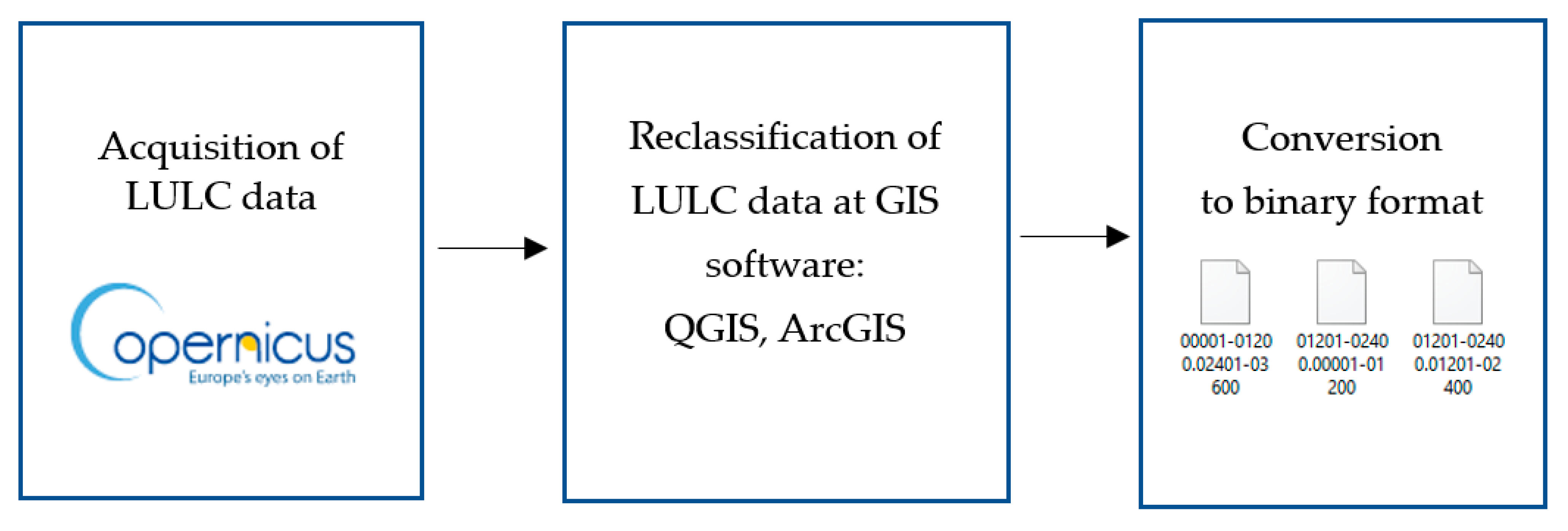
Figure 1. The procedure for implementing LULC data into the WRF model (based on Reference [28]).
Remotesensing 15 02389 g001
Figure 2. Visualization of LULC data for the Warsaw area from the: (a) CLC; (b) CGLS-LC100.
Remotesensing 15 02389 g002
Figure 4. Research area and areas of computing domains (D).
Remotesensing 15 02389 g004
Figure 5. Synoptic maps showing the analyzed synoptic situations at 12:00 UTC (based on Reference [63]) dated: (a) 22 June 2020—squall line; (b) 23 June 2020—occluded front; (c) 24 June 2020—occluded front; (d) 25 June 2020—squall line; (e) 26 June 2020—squall line.
Remotesensing 15 02389 g005aRemotesensing 15 02389 g005b
Figure 6. Examples of the results of daily temperature distributions from three variants of the model simulation on different geographical data and the results of measurements from meteorological stations (meteo stations) on 26 June 2020 at the analyzed meteorological stations: (a) Bielany; (b) Modlinska; (c) Most Polnocny; (d) Okecie.
Remotesensing 15 02389 g006
Figure 7. Examples of the results of wind distributions for 24 June 2020, 09:00 UTC from the model simulations on different geographical data: (a) CLC and SRTM; (b) CGLS and SRTM; (c) CLC and GMTED2010 (default topography); (d) MODIS and GMTED 2010 (default LULC and topography).
Remotesensing 15 02389 g007
Figure 8. Distribution of mean values of temperature forecast errors for the analyzed synoptic situations average over stations: (a) RMSE; (b) BIAS; (c) R.
Remotesensing 15 02389 g008
Figure 9. Distribution of mean temperature forecast errors at individual weather stations average over days: (a) RMSE; (b) BIAS; (c) R.
Remotesensing 15 02389 g009
Figure 10. Distribution of mean values of relative humidity forecast errors for the analyzed synoptic situations average over stations: (a) ME; (b) BIAS; (c) R.
Remotesensing 15 02389 g010
Figure 11. Distribution of mean relative humidity prediction errors at individual weather stations average over days: (a) ME; (b) BIAS; (c) R.
Remotesensing 15 02389 g011
Figure 12. Distribution of mean values of wind speed forecast errors for the analyzed synoptic situations average over stations: (a) RMSE; (b) BIAS; (c) R.
Remotesensing 15 02389 g012
Figure 13. Distribution of mean values of wind speed forecast errors at individual weather stations average over days: (a) RMSE; (b) BIAS; (c) R.
Remotesensing 15 02389 g013
Figure 14. Distribution of mean values of wind direction forecast errors for the analyzed synoptic situations average over stations: (a) ME; (b) BIAS; (c) R.
Remotesensing 15 02389 g014
Figure 15. Distribution of mean values of wind direction forecast errors at individual weather stations average over days: (a) RMSE; (b) BIAS; (c) R.
Remotesensing 15 02389 g015
Table 1. Reclassification procedure of CGLS-LC100 classes to MODIS classes.
LC-100 CodeLand Cover Class (CGLS-LC100)MODIS CodeMODIS Class
111Closed forest, evergreen needle leaf1Evergreen Needleleaf Forest
112Closed forest, evergreen broad leaf2Evergreen Broadleaf Forest
113Closed forest, deciduous needle leaf3Deciduous Needleleaf Forest
114Closed forest, deciduous broad leaf4Deciduous Broadleaf Forest
115Closed forest, mixed5Mixed Forest
116Closed forest, unknown3Deciduous Needleleaf Forest
121Open forest, evergreen needle leaf1Evergreen Needleleaf Forest
122Open forest, evergreen broad leaf2Evergreen Broadleaf Forest
123Open forest, deciduous needle leaf3Deciduous Needleleaf Forest
124Open forest, deciduous broad leaf4Deciduous Broadleaf Forest
125Open forest, mixed5Mixed Forest
126Open forest, unknown3Deciduous Needleleaf Forest
20Shrubs7Closed Shrublands
30Herbaceous vegetation10Grasslands
40Cultivated and managed vegetation/agriculture (cropland)12Croplands
50Urban/built up13Urban and Build-Up
60Bare/sparse vegetation16Barren or Sparsely Vegetated
70Snow and Ice15Snow and Ice
80Permanent water bodies21Lakes
90Herbaceous wetland 11Permanent Wetlands
100Moss and lichen16Barren or Sparsely Vegetated
200Open Sea17Water Bodies
0No input data available255Unclassified
Table 3. Coordinates list of locations of automatic weather stations of the City Cleaning Board.
No.Station NameCoordinatesNo.Station NameCoordinates
1Bielany52°17′32.675″N 20°58′22.367″E10Most Polnocny52°20′7.439″N
20°57′41.219″E
2Czecha52°13′32.231″N
21°9′57.347″E
11Plochocinska52°18′23.88″N 20°57′05.84″E
3Drewny52°7′38.892″N 21°5′48.407″E12Pulawska52°19′38.963″N 21°1′45.227″E
4Izbicka52°10′45.551″N 21°13′58.368″E13Radzyminska52°9′12.6″N 21°1′5.231″E
5Jelonki52°13′6.995″N
20°54′33.912″E
14Siekierkowska52°16′45.797″N 21°4′9.691″E
6Jerozolimskie52°12′14.615″N 20°56′26.555″E15Torwar52°12′9.252″N 21°3′57.887″E
7Krakowska52°10′30.719″N 20°56′39.803″E16Wilanow52°13′23.412″N 21°2′39.623″E
8Lazurowa52°14′46.5″N 20°53′52.044″E17ZOO52°15′14.147″N 21°1′19.596″E
9Modlinska52°20′7.439″N
20°57′41.219″E
18Zolnierska52°15′31.56″N 21°8′32.885″E
Table 4. The WRF model configuration used in the experiment for computational domains (D).
ParametersD1D2D3
Spatial resolution2.5 × 2.5 km500 × 500 m100 × 100 m
Surface layer schemeRevised MM5Revised MM5Revised MM5
Planetary boundary layer (PBL) schemeYSUnonenone
Radiation schemeRRTMGRRTMGRRTMG
MicrophysicsWSM6WSM6WSM6
Cumulusnonenonenone
Land surfaceNoahNoahNoah
Topographic datasetsSRTM/GMT2010SRTM/GMT2010SRTM/GMT2010
Land useCLC/CGLS-LC100/MODISCLC/CGLS-LC100/MODISCLC/CGLS-LC100/MODIS
Table 5. Average statistical evaluation of the simulations error values: ME, MAE, RMSE, MSE for five-day (22–27 June 2020) 24 h simulations for all stations (13 stations: 11 automatic and 2 airport stations) with 6 h spin-up time.
Average
Statistics
Model
Simulation
Temperature
(°C)
Relative Humidity
(%)
Wind Speed
(m/s)
Wind
Direction
(°)
Default0.98−11.292.1536.46
MECLC0.79−9.752.0121.79
CGLS0.85−10.312.1931.52
Default1.8015.072.2880.74
MAECLC1.6513.972.2276.43
CGLS1.6814.092.3576.20
Default2.2817.512.3999.12
RMSECLC2.1116.382.3590.99
CGLS2.1416.512.4692.49
Default6.03368.936.5712,415.11
MSECLC5.21324.566.3110,047.97
CGLS5.33331.326.9310,831.89
Table 6. Average statistical verification results (Pearson’s correlation coefficient (R), BIAS, and nRMSE) of the simulations for five-day (22–27 June 2020) 24 h simulations for all stations (13 stations: 11 automatic and 2 airport stations) with 6 h spin-up time.
Average
Statistics
Model
Simulation
TemperatureRelative HumidityWind SpeedWind
Direction
Default0.810.630.460.23
RCLC0.820.630.360.25
CGLS0.820.640.520.23
Default1.050.872.521.36
BIASCLC1.040.892.471.27
CGLS1.020.882.561.33
Default10.5822.75105.5467.72
nRMSE (%)CLC9.7721.28103.6762.17
CGLS9.9121.46108.4563.19
Table 7. Average statistical evaluation of error values: ME, MAE, RMSE, MSE for five-day (22–27 June 2020) 24 h simulations for two airport stations (spin-up time, 6 h).
Average
Statistics
Model
Simulation
Temperature (°C)Relative Humidity
(%)
Wind Speed
(m/s)
Wind
Direction
(°)
Default1.14−8.310.143.00
MECLC0.93−6.78−0.16−19.00
CGLS0.94−7.140.20−1.60
Default1.7212.710.6230.60
MAECLC1.6412.000.6832.00
CGLS1.6512.020.7433.00
Default2.1714.990.7939.66
RMSECLC2.0713.950.9243.09
CGLS2.0814.070.9340.63
Default5.52264.350.621611.40
MSECLC4.91219.660.851931.20
CGLS4.97223.480.901653.00
Table 8. Average statistical verification results (Pearson’s correlation coefficient, BIAS, and nRMSE) of the simulations for five-day (22–27 June 2020) 24 h simulations for all stations (13 stations: 11 automatic and 2 airport stations) with 6 h spin-up time.
Average
Statistics
Model
Simulation
TemperatureRelative HumidityWind SpeedWind
Direction
Default0.790.620.470.94
RCLC0.800.640.350.88
CGLS0.790.640.520.92
Default1.060.901.041.02
BIASCLC1.050.920.980.90
CGLS1.050.921.060.99
Default10.2419.9318.3321.29
nRMSE (%)CLC9.7518.5421.3623.13
CGLS9.8218.7021.5521.81
Disclaimer/Publisher’s Note: The statements, opinions and data contained in all publications are solely those of the individual author(s) and contributor(s) and not of MDPI and/or the editor(s). MDPI and/or the editor(s) disclaim responsibility for any injury to people or property resulting from any ideas, methods, instructions or products referred to in the content.