Article

Differential Settlement of Track Foundations Identification Based on GRU Neural Network

1
Department of Civil Engineering, Hangzhou City University, Hangzhou 310015, China
2
College of Civil Engineering and Architecture, Zhejiang University, Hangzhou 310058, China
3
Center for Balance Architecture, Zhejiang University, Hangzhou 310058, China
*
Author to whom correspondence should be addressed.
Remote Sens. 2023, 15(9), 2378; https://doi.org/10.3390/rs15092378
Submission received: 12 March 2023 / Revised: 23 April 2023 / Accepted: 27 April 2023 / Published: 30 April 2023
(This article belongs to the Special Issue Remote Sensing in Civil and Environmental Engineering)

Abstract

:
The timely identification of differential settlement of track foundations is of great significance for the safety of train operation and the maintenance of track structures. However, traditional monitoring techniques cannot meet the requirements of efficient, real-time, and automatic monitoring of track foundation settlement. In order to solve these problems, a real-time identification method based on a gated recurrent unit (GRU) neural network is proposed for the differential settlement of track foundations monitoring. According to parameter sensitivity analysis, the vertical acceleration of the vehicle is selected as the known data fed into the GRU network for differential settlement identification. Then the GRU network is employed to establish the nonlinear relationship between the vertical acceleration of the vehicle and the differential settlement of the track foundation. The results indicate that the longitudinal continuous differential settlement distribution curve of track foundations could be accurately identified with GRU neural network through the real-time vibration response of the vehicle–track. The current method may provide a new means for the real-time and efficient identification of the differential settlement of track foundations.

1. Introduction

The differential settlement of the track foundation will cause an internal force change and vertical profile irregularity of the track structure [1,2], which will adversely affect the safety of the train operation and the comfort of passengers. The differential settlement of the track foundation will drive the following settlement of each track structure [3]. When the train passes through the deformed track, the vehicle body vibration response and track structure stress increase significantly [4]. The amplitude and wavelength of foundation settlement and the train speed have obvious effects on the vehicle–track dynamic response [5,6]. On the one hand, differential settlement of the track foundation will cause deformation and additional stress in the track structure, which will lead to structural damage; on the other hand, it will lead to a decline in its service performance, which will have a negative impact on riding comfort and safety [7,8]. Therefore, as a common problem in railway and urban rail transit, long-term monitoring of the differential settlement of track foundations is of great significance to the daily safe maintenance of track infrastructure.
The traditional foundation deformation monitoring method is a classic ground measurement method that uses traditional measuring instruments such as level, theodolite, and electronic total stations [9,10]. These traditional monitoring methods can only work when the train is stopped, and they consume manpower. They can only be used as regular detection means, and it is difficult to realize the long-term real-time perception of track foundation settlement. With the development of electronic communication technology, global positioning system (GPS) measurement [11], static level measurement [12], synthetic aperture (differential) radar interferometry (InSAR, D-InSAR) [13,14], optical fiber sensing technology [15,16] and so on have been successively applied to foundation settlement monitoring. These technologies can meet the monitoring needs to a certain extent, but the use cost is relatively high, and the monitoring process is highly dependent on equipment.
With the advent of the big data era and the development of artificial intelligence technology, many scholars have proposed intelligent algorithm models to solve engineering problems [17,18,19,20,21], including studies on differential foundation settlement prediction. Tian [22] established the prediction model of vertical displacement (settlement) deformation based on the GM (1,1) model and proved that the grey theory model is applicable to the prediction analysis of settlement deformation. However, the above GM (1,1) model is a single-point prediction model, which cannot consider the settlement correlation between discrete monitoring points and cannot reflect the overall deformation law of the foundation. Therefore, Liu et al. [23] expanded the single point GM (1,1) model to a multivariable grey model (MGM (1, n)), realizing the overall prediction of multipoint monitoring deformation. Li et al. [24] successfully predicted the settlement of soft soil subgrade by using an artificial neural network (ANN) model based on field-measured data and verified that the ANN model is superior to the traditional method. Furthermore, to improve the prediction precision, network models such as the wavelet neural network (WNN), long short memory neural network (LSTM), gated recurrent unit (GRU) neural network, and one-dimensional convolutional neural network (Conv1d) have also been used for settlement deformation prediction [25,26]. However, most of the current research focuses on the prediction of subgrade or building foundation settlement, and research on the prediction of track foundation settlement is limited. Zhu et al. [27] built a grey neural network model based on the characteristics of the grey model and neural network and successfully predicted the differential settlement of the Nanjing subway tunnel. LIANG et al. [28] carried out Markov correction on the basis of unbiased optimization of the grey model based on the monitoring data of railway foundation settlement, which improved the prediction precision. The above research [27,28] has achieved good results with respect to the prediction of track foundation settlement, but all of them use the existing foundation settlement data to predict the settlement development trend of a single point location and are unable to obtain a continuous settlement distribution curve along the track direction, and have difficulty achieving real-time status monitoring of foundation settlement.
In this paper, a real-time monitoring strategy for the track foundation settlement based on an intelligent algorithm is proposed. In the process of realizing this, there are two major difficulties to be solved: (1) Analysis of sensitive vibration indexes: among the numerous vehicle–track dynamic response indexes, which dynamic response index is sensitive to the track foundation settlement and suitable for identifying the differential settlement of the foundation; (2) Intelligent identification of differential settlement of track foundation based on sensitive vibration indexes: Using which method to obtain real-time longitudinal continuous settlement distribution from sensitive dynamic response indexes. In view of the above difficulties, a train–monolithic bed track system model is established. The abnormal vehicle–track dynamic responses when the train passes through the differential settlement section of the track foundations are analyzed, and then the dynamic response indexes that are sensitive and regular to the foundation settlement are obtained. To obtain the real-time longitudinal continuous distribution of track foundation settlement, the vehicle–track dynamic response used to identify the track foundation settlement is the corresponding time series data, and the recurrent neural network has obvious advantages in processing the time sequence data. However, the traditional recurrent neural network may have the problem of gradient explosion and gradient disappearance [29], so the GRU neural network is employed to overcome this problem. In conclusion, a real-time identification method is proposed in this paper for the differential settlement of track foundations based on a GRU neural network. The advantage of this method is that the real-time longitudinal continuous settlement distribution of the track foundation can be obtained only by the real-time dynamic response data obtained by the track inspection train without the aid of complex technology and equipment.

2. Methods

In this paper, a real-time identification method of track differential foundation settlement based on a GRU neural network is proposed. The research process of the method is divided into two steps: (1) Analysis of sensitive vibration indexes: many abnormal dynamic responses will be generated through vehicle–track system when the train passes through the differential foundation settlement area. Then the vehicle–track dynamic response indexes sensitive to foundation settlement can be found; (2) The GRU neural network is used to deeply excavate the hidden nonlinear relationship between the vehicle–track vibration response easily obtained and differential settlement of the track foundation difficult to measure. In order to obtain the sensitive vehicle–track dynamic response suitable for GRU neural network model learning and training, the train–monolithic bed track system is first established, then the sensitive and regular dynamic response indexes to track foundation settlement are obtained after analysis from many vehicle–track dynamic responses, and a database containing the indexes and the corresponding track foundation settlement is constructed. Furthermore, the GRU neural network model is established and trained with the time series data of “settlement value-sensitive indexes “. The hidden nonlinear relationship between the vehicle–track vibration response and differential settlement of the track foundation will be established when the GRU network is well-trained (Figure 1).

2.1. Analysis of Sensitive Vibration Indexes

To obtain sensitive and regular dynamic response indexes to track foundation settlement and theoretical database data, the commonly used two-dimensional analysis model of the train–monolithic bed track system is adopted in this paper, as shown in Figure 1a. The differential settlement for different types of track foundations only influences the numerical values and variation patterns of the vehicle–track dynamic response, but the dynamic response of vehicle–track is also closely related to the differential settlement of track foundation, and the GRU neural network model is used to identify the differential settlements of track foundation based on the mapping relationship between the vehicle–track dynamic response and the differential settlements of track foundation, therefore, the method in this study can also be used to identify differential settlements for other types of track foundations. The motion equation and main calculation parameters of the train and track of the train–monolithic bed track system can be found in Jiang et al. (2020) [30]. The train adopts a double metro B-type train, with a total length of 38 m, the length of the track and monolithic track bed l r is 320 m, and the train operation section is 40–320 m. The type of fasteners is DTVI2-1, with an interval of 0.625 m, and a total of 512 fasteners are laid under the track. The train running speed refers to the daily running speed of the subway, which is 20 m/s, 25 m/s, and 32 m/s.
Since the calculation results of this model will be used for the subsequent study on differential settlement identification of foundations, to improve the persuasiveness of the results of this paper, the actual conditions should be simulated as much as possible when establishing the model. In reality, the mass of the train will change with the number of passengers, and the number of fully loaded passengers in a single compartment of metro B-type train is 240. The train mass is the empty train mass plus the passenger mass. The number of passengers is a random integer between 0 and 240, and the average passenger mass is 60 kg. The stiffness and damping of various components involved in the vehicle–track system also have a certain difference around the standard value, such as primary suspension, secondary suspension, fasteners, etc. In this paper, the random error value of ±2% is considered for the stiffness and damping coefficient of each component in the calculation model, and the error follows the standard normal distribution. The track random irregularity is set according to the American Level VI irregularity spectrum, as shown in Formula (1). The random irregularity of the track is recorded as r1(x).
S v ( Ω ) = k · A v · Ω c 2 Ω 2 Ω 2 + Ω c 2
where Ω is the space angular frequency of track irregularity; Ω c is the cut-off frequency; k is the safety factor, which is 0.25 here; and A v is the roughness coefficient, which is 0.0339.
The track foundation settlement is mostly concave cosine settlement [30], and the track structure will have corresponding vertical deformation with the differential settlement of the foundation. The smaller the ratio of the settlement amplitude h 0 and the settlement wavelength λ 0 , the more closely the following deformation of the track structure conforms to the foundation settlement. In this paper, the train operation section is 40~320 m, and the differential foundation settlement center is set at the midpoint of the operation section, which is 180 m from the track. The differential foundation settlement model is introduced, as shown in Figure 1b, and the cosine settlement follows Formula (2). The following assumptions are made for the model: 1. When h 0 (mm)/ λ 0 (m) ≤ 1, the track will have a complete following settlement, and the deformation is consistent with the foundation settlement; 2. All supporting elements are intact without damage or separation from the track structure; 3. The following deformation of the track caused by the differential settlement of the foundation is taken as the initial condition; then, the initial condition of track deformation is r(x) = r1(x)+ h(x).
h ( x ) = 0 , x < x 0 , x > x 0 + λ 0 h 0 2 1 cos 2 π x x 0 λ 0 , x 0 x x 0 + λ 0
where h 0 is the amplitude of foundation settlement; λ 0 is the wavelength of foundation settlement; and x 0 is the coordinate of the starting point of settlement. In this model, the amplitude range is 5~100 mm and the interval is 5 mm; the wavelength range is 20~100 m, the interval is 20 m, and h 0 (mm)/ λ 0 (m) ≤ 1; running speed v 0 of the model train in this paper is set as 20 m/s, 25 m/s, 32 m/s.

2.2. Identification Study Based on the GRU Neural Network

The numerical results from the above train–monolithic bed track system can be analyzed to obtain dynamic response indexes that are regular and sensitive to the settlement of the track foundation. The sensitive dynamic response will be used as the characteristic to identify track foundation settlement. Because the vehicle–track dynamic response is the corresponding time series data, and the GRU neural network model has significant advantages in training time series data, through good training and parameter optimization, it can realize real-time identification of the longitudinal continuous foundation settlement depth along the track from the vehicle rail dynamic response. The specific identification process is shown in Figure 1c, which is divided into three steps: (1) database establishment; (2) network configuration and training; and (3) model validation.
In step 1, the database is divided into a theoretical simulation database and an engineering measurement database. The theoretical database is derived from the sensitive vehicle–track dynamic response value R 0 obtained from the theoretical simulation of the metro train–monolithic bed track system in the Section 2.1 and the corresponding train running speed v 0 and settlement depth h 0 of the track foundation. The measured database is the engineering-measured data composed of the same elements as the theoretical database. Each database is divided into a training dataset, verification dataset, and test dataset. Among them, the training set is used for training the model. The validation set preliminarily evaluates the model and continuously adjusts the super parameters until the model reaches the optimum. The test set is used to evaluate the generalization capability of the final model. First, the GRU neural network model is trained with the theoretical simulation database to identify the settlement state of the track foundation, and the theoretical feasibility of this method is verified. After that, the model is verified by using the measured database to prove the applicability of the method in engineering practice.
In step 2, the GRU neural network is constructed and trained with the database established above. The GRU neural network consists of an input layer, a gating neural unit (GRU) layer, and a fully connected layer (Figure 1c). During the training, the known time series data of the sensitive dynamic response value R 0 , corresponding train running speed v 0 , and settlement depth h 0 of the track foundation to be identified are first fed into the GRU layer through the input layer and continuously update the weight in the GRU layer to fully excavate the nonlinear correlation between R 0 , v 0 and h 0 . When the training precision is reached MSE ≤ 0.01(formula (7)), the weight update is ended, and the result is output to the fully connected layer. In this process, the update gate in the GRU layer controls the degree to which the state information of the relationship between R 0 , v 0 and h 0 learned and trained at the previous time h t 1   is brought into the current state, and the reset gate in the GRU layer controls the degree to which the state information of the previous time h t 1   is written into the current time state h t . The existence of an update gate and reset gate reduces the possibility of training overfitting. The output formulas are:
z t = σ W z x t + U z h t 1
r t = σ W r x t + U r h t 1
The output of GRU hidden layer neurons can be expressed as:
h ˜ t = tanh W A x t + U λ r t × h t 1
h t = 1 z t × h t 1 + z t × h ˜ t
where z t is the output of the update gate, r t is the output of the reset gate, σ is the sigmoid function, x t is the input characteristic at time t, h t , h t 1 is the hidden state at time t and time t−1, h ˜ t is the active state at time t, and W z , U z , W r , U r , W A , and U λ are the weights of the corresponding gates.
In step 3, three indexes are selected to evaluate the model: normalized root mean square error (nRMSE), mean absolute percentage error (MAPE), and determination coefficient (R2). The first two indexes indicate the dispersion degree of the deviation between the predicted value and the true value; the larger the value is, the worse the prediction effect. R2 indicates the degree of fit between the predicted value and the true value; the larger the value is, the higher the overall prediction precision. The indexes are defined as follows:
M S E = i = 1 m y i y ^ i 2
n R M S E = 1 m i = 1 m y i y ^ i 2 y ¯ × 100 %
M A P E = 100 % m i = 1 m y i y i ^ y i
R 2 = 1 i = 1 m y i y ^ i 2 i = 1 m y i y ¯ 2
where m is the number of samples; y ^ i and y i   are the predicted value and the true value, respectively; and y ¯ is the average value of the sample.

3. Results and Discussion

3.1. Analysis of Sensitive Vibration Indexes

One of the difficulties in this paper is to find the vehicle–track dynamic response indexes that are regular and sensitive to track foundation settlement. When differential settlement of the foundation occurs, the dynamic response of the vehicle and track will change significantly with the change in train speed v 0 , settlement wavelength λ 0 and amplitude h 0 . Among various vehicle–track dynamic responses, the changes in the vertical acceleration of the vehicle a c and the wheel–rail contact force F w r are obvious and the most regular, which are ideal dynamic response indexes to identify the differential settlement of the track foundation. Therefore, the vertical acceleration of the vehicle a c and the wheel–rail contact force F w r are mainly analyzed here.
(1)
The vertical acceleration of the vehicle   a c
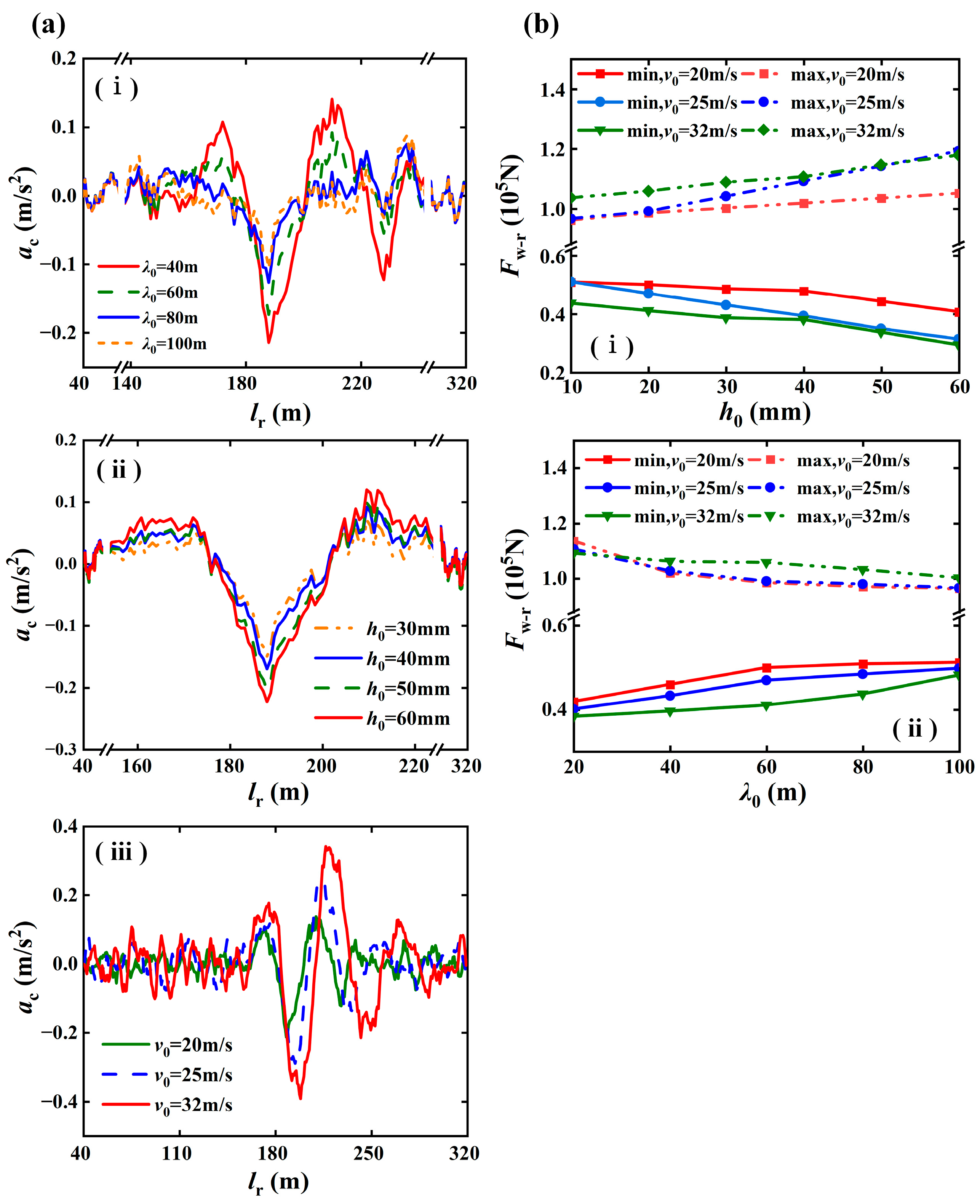
When the differential settlement waveform of the foundation changes, the vertical acceleration of the vehicle is obviously affected by the change in the settlement wavelength and amplitude, but the overall trend and regularity are basically consistent, as shown in Figure 2a. When the train enters the settlement section, the vertical acceleration of the vehicle increases in the positive direction first. Then, it negatively increases rapidly to the maximum, but the position of the maximum negative value is behind 180 m of the track, indicating the delayed expression of the vertical acceleration of the vehicle for foundation settlement. When the train is about to leave the settlement section, the vertical acceleration of the vehicle is still significantly increased compared with the nondifferential settlement of the track.
When studying the influence of the settlement wavelength on the vertical acceleration of the car body, keeping the train running speed at 20 m/s and the settlement amplitude at 40 mm, the settlement wavelengths are 40 m, 60 m, 80 m, and 100 m, and the results are shown in Figure 2a(i). With increasing settlement wavelength, the vertical acceleration of the vehicle decreases gradually. When the wavelength changes from 40 m to 100 m, the negative maximum vertical acceleration of the vehicle changes from 0.2198 m/s2 to 0.1126 m/s2, decreasing by 48.7%. The maximum positive value of 0.1436 m/s2 becomes 0.0951 m/s2, decreasing by 33.8%.
The influence of the wave amplitude on the vertical acceleration of the vehicle is shown in Figure 2a(ii). The speed of the train is 20 m/s, the settlement wavelength is 60 m, and the settlement amplitudes are 30 mm, 40 mm, 50 mm, and 60 mm. When the amplitude of the settlement wave increases, the vertical acceleration of the vehicle increases. When the wave amplitude increases from 30 mm to 60 mm, the amplitude of the vertical acceleration of the vehicle increases by 65.7%.
The train speed also has an important influence on the vertical acceleration of the vehicle. Assuming that the settlement wavelength is 40 m, the amplitude is 40 mm, and the train speeds are 20 m/s, 25 m/s, and 32 m/s, the results are shown in Figure 2a(iii). With increasing train speed, the trend of the vertical acceleration of the vehicle curve is basically consistent, but the maximum value increases significantly. When the running speed of the train increases from 20 m/s to 32 m/s, the extreme value of the vertical acceleration of the vehicle increases from 0.2246 m/s2 to 0.4023 m/s2, with an increase of 79.1%. The running speed of the train has a significant impact on the dynamic response of the train. Therefore, the speed of the train shall be reduced as much as possible when passing through the differential settlement section.
(2)
The wheel–rail contact force   F w r
When the train passes the differential foundation settlement section, the wheel–rail contact force is also sensitive to the foundation settlement. Generally, research on the wheel–rail contact force only focuses on the minimum because if it is too small, the danger of train derailment may occur. However, the ultimate purpose of this paper is to identify the settlement of the track foundation and to understand the complete law of the wheel–rail contact force, so the maximum value is also included in the scope of discussion.
In this paper, the influence of the settlement amplitude on the wheel–rail contact force is studied first. Assuming that the settlement wavelength is 60 m and the settlement wave amplitudes are 10 mm, 20 mm, 30 mm, 40 mm, 50 mm, and 60 mm, the results are shown in Figure 2b(i). With increasing settlement amplitude, the maximum value of the wheel–rail contact force gradually increases, and the minimum value gradually decreases. The maximum and minimum values have a trend of symmetry with respect to the central value. When the wavelength changes from 10 mm to 60 mm, and the train speed is 20 m/s, 25 m/s, and 32 m/s, the maximum value increases by 9.8%, 23.5%, and 13.5%, respectively, and the minimum value decreases by 20%, 38.7%, and 32.4%, respectively. The change amplitude of the minimum value is significantly greater than that of the maximum value.
When studying the influence of the settlement wavelength on the wheel–rail contact force, we kept the settlement wave amplitude unchanged at 20 mm, and the settlement wavelengths are 20 m, 40 m, 60 m, 80 m, and 100 m; the results are shown in Figure 2b(ii). With increasing settlement wavelength, the maximum value of the wheel–rail contact force gradually decreases, and the minimum value gradually increases, indicating that the overall vibration of the wheel–rail contact force becomes increasingly weaker. When the wavelength changes, the change rates of the maximum value and minimum value are different at different speeds. When the wavelength changes from 20 m to 100 m, and the train speeds are 20 m/s, 25 m/s, and 32 m/s, the maximum value decreases by 15.1%, 12.8%, and 8.1%, respectively, and the minimum value increases by 22.3%, 24.4%, and 25.8%, respectively.
As shown in Figure 2b, under the same settlement wavelength and amplitude, with increasing train speed, the maximum value of the wheel–rail contact force gradually increases, the minimum value gradually decreases, and the change amplitude is obvious, but the change law is not a simple linear change, and the changing trend is not strictly the same: when the wavelength is 20 m (Figure 2b(i)), and when the wave amplitude is 60 mm (Figure 2b(ii)), the maximum value does not strictly follow the law of change with speed, which may be related to the randomness of the stiffness and damping values of each track element in the model. Therefore, it is not feasible to judge the foundation settlement only by the maximum and minimum values, and the complete wheel–rail force time-history curve is the basis for subsequent identification of foundation settlement.
Based on the above analysis, it is found that the vertical acceleration of the vehicle and the wheel–rail contact force are sensitive to the differential settlement of the track foundation. To further analyze sensitive vibration indexes, the close relationship between the vertical acceleration of the vehicle, the wheel–rail contact force, and the differential settlement of the track foundation is verified, and the coherence function was introduced:
γ x y 2 = S x y 2 ( k ) S x x ( k ) S y y ( k ) 0 γ x y 2 1
where γ x y 2 is the coherence function value; S x x ( k ) , S y y ( k ) are the self-power spectral density functions of the two signals respectively; S x y 2 ( k ) is the cross-power spectral density function of the two signals.
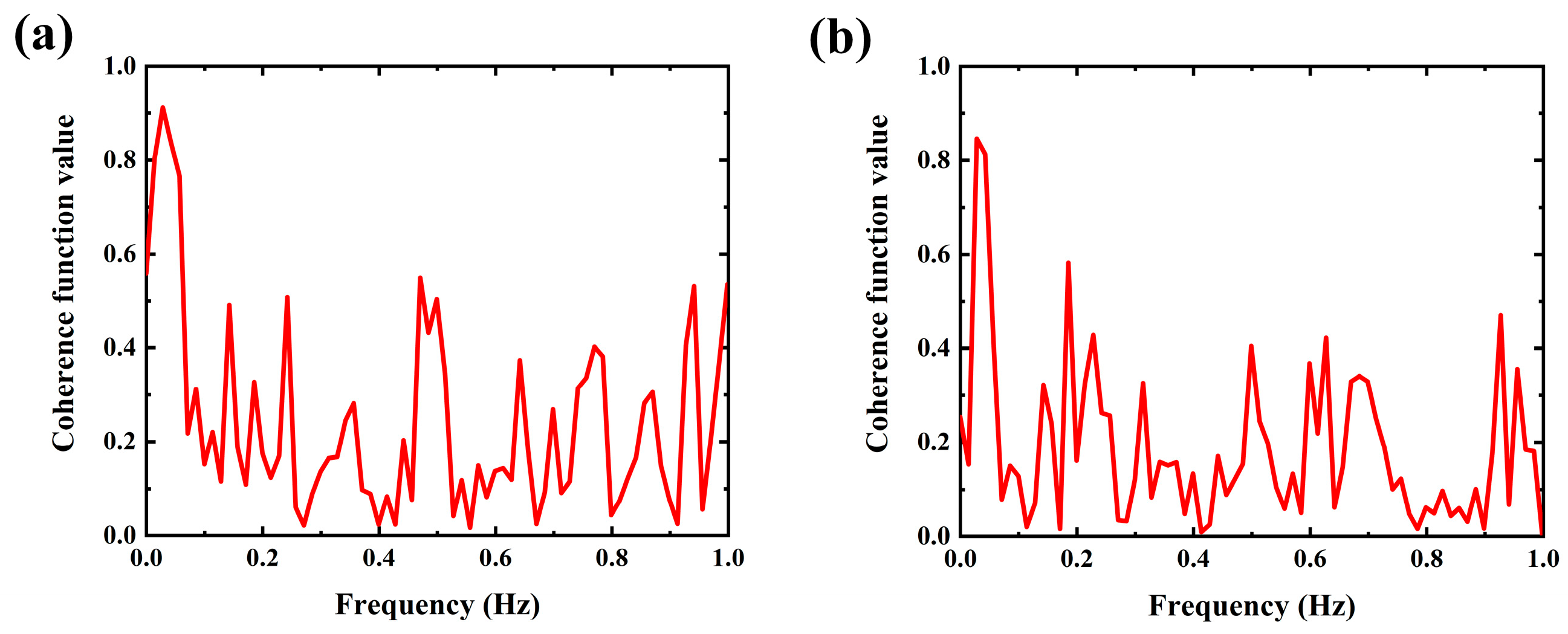
The causal relationship between the two signals can be well analyzed by coherence analysis, so it can be used to verify the impact of the differential settlement of the track foundation on the vertical acceleration of the vehicle and the wheel–rail contact force. The larger the coherence function value, the closer the relationship between the two signals; generally, when 1 / 2 γ x y 2 1 , we believed that the two signals have high coherence. In the analysis of the coherence between the vertical acceleration of the vehicle, the wheel–rail contact force, and the differential settlement of the track foundation, 12 sets of settlement conditions are selected to construct samples when the train speed is 20 m/s, and the settlement wavelength is 60 m. The coherence calculation results are shown in Figure 3. It can be seen that the values of the coherence function between the vertical acceleration of the vehicle, the wheel–rail contact force, and the differential settlement of the track foundation are greater than 0.5 in the low-frequency range, and the maximum coherence function value of the vertical acceleration of the vehicle reaches 0.911, which is obviously greater than 0.845 of the wheel–rail contact force, indicating that the coherence between t the vertical acceleration of the vehicle and the differential settlement of the track foundation is higher.
In summary, the vertical acceleration of the vehicle and the wheel–rail contact force are not only very sensitive to the differential settlement of the track foundation but also closely related. Therefore, in a subsequent study, the vertical acceleration of the vehicle and the wheel–rail contact force will be used as sensitive vibration indexes to identify differential settlement of the track foundation.

3.2. Verification of the Differential Settlement Identification Method

To verify the feasibility and precision of the proposed method for differential settlement identification from the measured vertical acceleration of the vehicle and the wheel–rail contact force, numerical simulations and comparative analysis to actual site conditions are evaluated.

3.2.1. Complete Settlement Waveform of a Single Velocity Group

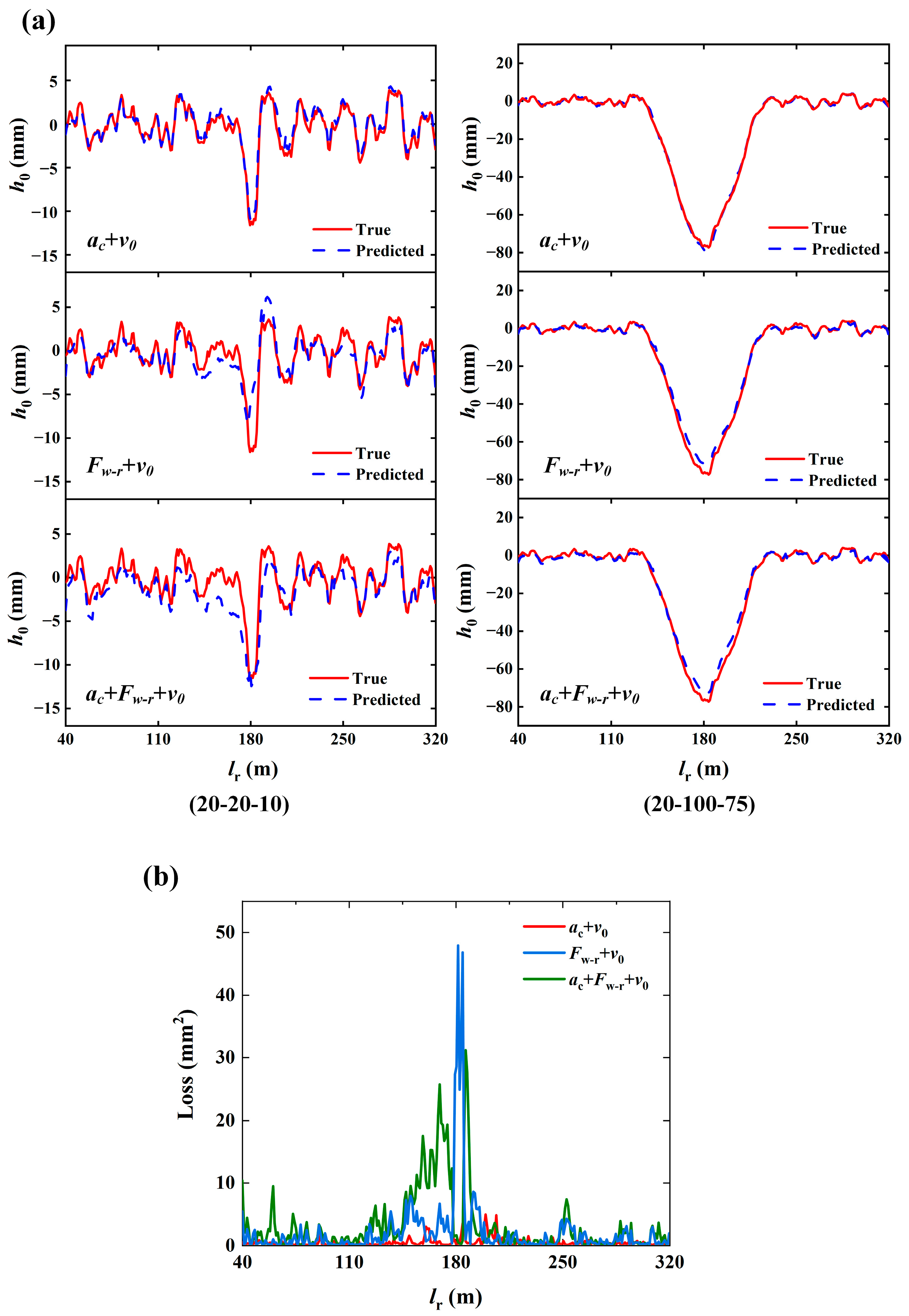
The settlement condition with a train running speed of 20 m/s is selected as the sample data, and each group of data consists of a complete settlement waveform (i.e., track 40–320 m) and its corresponding dynamic response time-history data. In order to confirm the most suitable dynamic response indexes for identifying the track foundation settlement, the input is divided into three combinations: (1) two-dimensional time sequence data composed of the vertical acceleration of the vehicle and train running speed are taken as the input; (2) the two-dimensional time sequence data composed of the wheel–rail contact force and train running speed are taken as the input; and (3) the three-dimensional time sequence data composed of the vertical acceleration of the vehicle, the wheel–rail contact force, and train running speed are taken as the input. All outputs are complete settlement waveforms. Comparing the identification results of three different input combinations, we randomly select the identification results of 20-20-10 (speed is 20 m/s, settlement wavelength is 20 m, and amplitude is 10 mm; the same below) and 20-100-75 in the test set as examples, as shown in Figure 4a; the identification results are evaluated by nRMSE, MAPE, and R2, as shown in Table 1. To quantitatively evaluate the performance of the GRU neural network, the identification results of 20-100-75 (when the input is combination (1)) are taken as an example to analyze specifically. The nRMSE reflects the stability of the identification by the GRU neural network. The nRMSE of the identified settlement values is only −2.4%, which indicates the high stability in Settlement identification by the GRU neural network, and the MAPE reflects the relative ratio of the identification error; the MAPE of the identified settlement values is 13.8%. The relatively large MAPE is caused by the large dispersion of the deviation between the predicted values and the true values in the two ends of the settlement area, but there is still a high precision in overall settlement identification by the GRU neural network. In addition, the R2 reflects the fitting degree between the identified settlement values and the true settlement values. The R2 of the identified results is 0.99832, which is very close to 1, indicating the high consistency of overall settlement distribution. Above all, it can be found that the differential settlement of the track foundation can be well identified by the GRU neural network. However, the identification precision is far better than the other two combinations when the two-dimensional time sequence data composed of the vertical acceleration of the vehicle and the train speed are used as the input. Specifically, when the two-dimensional time sequence data composed of the wheel–rail contact force and train speed are taken as the input, nRMSE and MAPE increase to −9.0% and 28.1%, respectively, and R2 decreases to 0.98203, which indicates a significant decrease in stability of the identification and consistency of overall settlement distribution. When the three-dimensional time sequence data composed of the vertical acceleration of the vehicle, the wheel–rail contact force, and train running speed are taken as the input, the identification effect is between the two input combinations, indicating that when the input includes the wheel–rail contact force, the identification precision will decrease. For the identification results of 20-20-10, the above conclusion can also be drawn. It is mainly because the wheel–rail contact force is more sensitive to the variation in the stiffness and damping of each track element. In reality, the stiffness and damping of each track element will change due to deterioration. Therefore, the wheel–rail contact force is not suitable as input data in differential settlement identification of track foundations. In subsequent research, the input is all two-dimensional time sequence data composed of the vertical acceleration of the vehicle and train running speed.
In addition, comparing the output results of 20-20-10 and 20-100-75 under the same situation, it is found that the identification precision is low when the settlement depth is small. Taking the identification results as an example, when the time sequence data composed of the vertical acceleration of the vehicle and train speed are taken as the input, compared to the identification results of 20-100-75, the evaluation indicators nRMSE and MAPE of the identification results of 20-20-10 increase to −12.9% and 17.9% respectively; Correspondingly, the determination coefficient R2 decreases to 0.93751, which indicates that the identification precision of 20-20-10 is significantly lower than that of 20-100-75. When comparing the results of other input combinations, the same conclusion can be drawn. The precision of the model in identifying small amplitude settlements is significantly lower than that of large amplitude settlements, mainly because the magnitude of small amplitude settlement is similar to the random irregularity of the track, resulting in a decrease in identification precision. In order to further confirm the error size of the model in identifying small amplitude settlements (20-10), Figure 4b shows the spatial error distribution of the identification results under three input combinations, and the error calculation method is shown in Equation (12).
L o s s = y i y ^ i 2
From Figure 4b, it can be observed that the prediction values of 20-20-10 have a significant error when the input includes the wheel–rail contact force. When the input is the time sequence data composed of the vertical acceleration of the vehicle and train speed, the significant error mainly exists near the settlement center, with a maximum error of only 2.21 mm; Based on the identification results of the overall settlement trend in Figure 4a of 20-20-10, it is found that the model can also achieve a good precision in identifying settlement areas. Therefore, although the GRU neural network model is slightly inferior in identifying small amplitude settlements compared to large amplitude settlements, it is equally applicable.

3.2.2. Complete Settlement Waveform of the Mixing Velocity Group

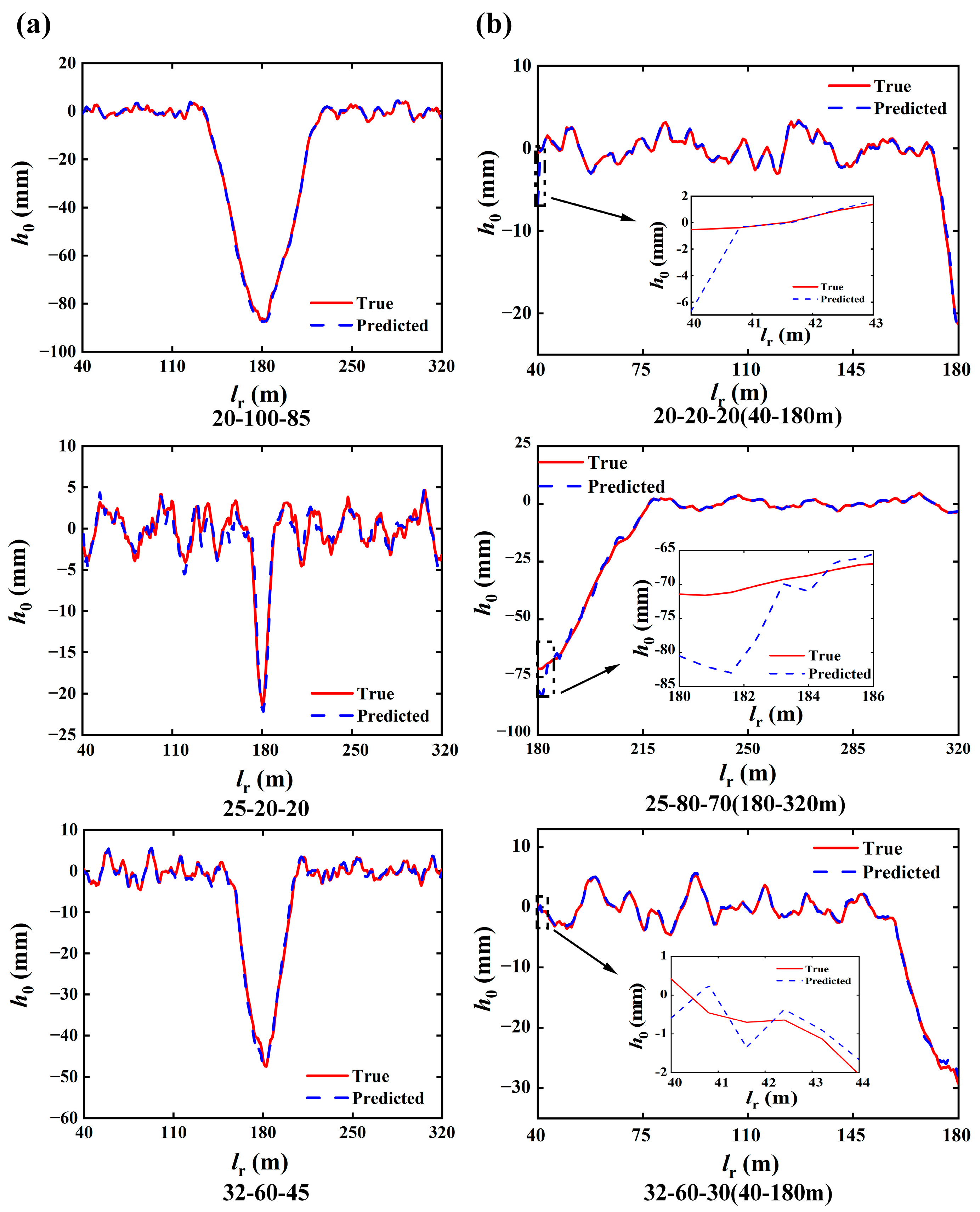
Considering the change in train speed in reality, this section selects each settlement condition with train running speeds of 20 m/s, 25 m/s, and 32 m/s as the sample data. Each group of data consists of a complete settlement waveform and the corresponding vertical acceleration of the vehicle time-history data. The two-dimensional time sequence data composed of the vertical acceleration of the vehicle and the running speed of the train are taken as the input, and the output is a complete settlement waveform. The identification results of 20-100-85, 25-20-20, and 32-60-45 in the test set are randomly selected as examples, as shown in Figure 5a, and the evaluation index is shown in Table 2. When comparing Figure 4 and Figure 5a, Table 1 and Table 2, it can be concluded that: the model has good precision in identifying the differential settlement of the track foundation at different train speeds by using the vertical acceleration of the vehicle, but the overall identification precision is slightly inferior to the identification results of a single speed group. Specifically, when the input is maintained to be the time sequence data composed of the vertical acceleration of the vehicle and train speed, in identifying the complete settlement waveform of a single speed group, the average values of nRMSE, MAPE, and R2 for the two output conditions are −7.7%, 15.9% and 0.96792 respectively; While in identifying complete settlement waveform of the mixing velocity group, the average values of nRMSE and MAPE with similar settlement sizes increase to −9.3% and 18.9% respectively, the average value of R2 decreases to 0.96158, which indicate that there is a significant decrease in both stability of the identification and consistency of overall settlement distribution. It is mainly because the variation in train speed increases the complexity of vehicle–rail dynamic response, leading to a significant decrease in identification precision. Therefore, if the vertical acceleration of the vehicle time-history data is used to identify the differential settlement of the track foundation in reality, the train should be driven at a uniform speed as much as possible.

3.2.3. One-Half Settlement Waveform of the Mixing Velocity Group

The above identification studies on the differential settlement of track foundations are all based on complete settlement waveforms, but in actual identification, differential settlement is not necessarily a complete settlement waveform. Therefore, in this section, each settlement condition with train speeds of 20 m/s, 25 m/s, and 32 m/s is selected as the sample data. Each group of data consists of 1/2 of the settlement waveform (i.e., track 40–180 m or 180–320 m) and its corresponding vertical acceleration of the vehicle time-history data. The two-dimensional time sequence data composed of the vertical acceleration of the vehicle and the train running speed are taken as the input, and the output is a 1/2 settlement waveform. The identification results of 20-20-20 (40–180 m), 25-80-70 (180–320 m), and 32-60-30 (40–180 m) in the test set are randomly selected as examples, as shown in Figure 5b, and the evaluation indexes are shown in Table 3. It is found that the model is also effective in identifying the 1/2 settlement waveform. Specifically, the average values of nRMSE, MAPE, and R2 for the three output conditions are −8.2%, 20.3%, and 0.98924, respectively, and all error evaluation indexes are in a relatively ideal range. However, in the identification of 20-20-20 (40–180 m) and 25-80-70 (180–320 m), a large error is observed in the identification starting point; the maximum errors are 6.1 mm and 10.4 mm, respectively; In 32-60-30 (40–180 m) identification, the maximum error is only 0.65 mm, the precision of starting point identification was significantly higher than that of the other two groups. Since the setting range of the settlement wavelength in this paper is 20~100 m, and the amplitude is 5~100 mm, 32-60-30 is in the middle of the whole settlement sample compared with the other two groups, so the samples on both sides are even and more, which makes the identification precision of the starting point higher. This shows that when there are enough sample data, the GRU neural network can overcome the disadvantage of large errors in starting point identification to some extent. In reality, to avoid a large starting point identification error of the GRU neural network, the time step of data input can be appropriately increased.

3.2.4. Engineering Measurement Verification

In order to prove the applicability and feasibility of the above methods, the data of 12.2 km to 12.7 km track settlement deformation and the corresponding vertical acceleration of a vehicle of a certain railway in China are selected for analysis and verification, as shown in Figure 6a. The study section is 500 m long in total, with the first 450 m as the training set and verification set and the last 50 m as the test set. The identification results are shown in Figure 6b; the error evaluation indexes nRMSE, MAPE, and R2 are 17.3%, 15.1%, and 0.83134, respectively (Table 4). The model can basically identify the trend of track deformation, but some obvious distinctions are still observed between the rail deformation of identification and application in some areas, mainly because there are too few sample data. In other words, the identification precision of the engineering-measured data is sufficient to illustrate the feasibility and applicability of the method.

3.3. Discussion

The hyperparameters in the neural network model have a great influence on the identification precision. Herein, the effects of the hidden neurons quantity and learning rate of GRU on identification precision and training efficiency are discussed [31].

3.3.1. Effect of the Quantity of Hidden Neurons

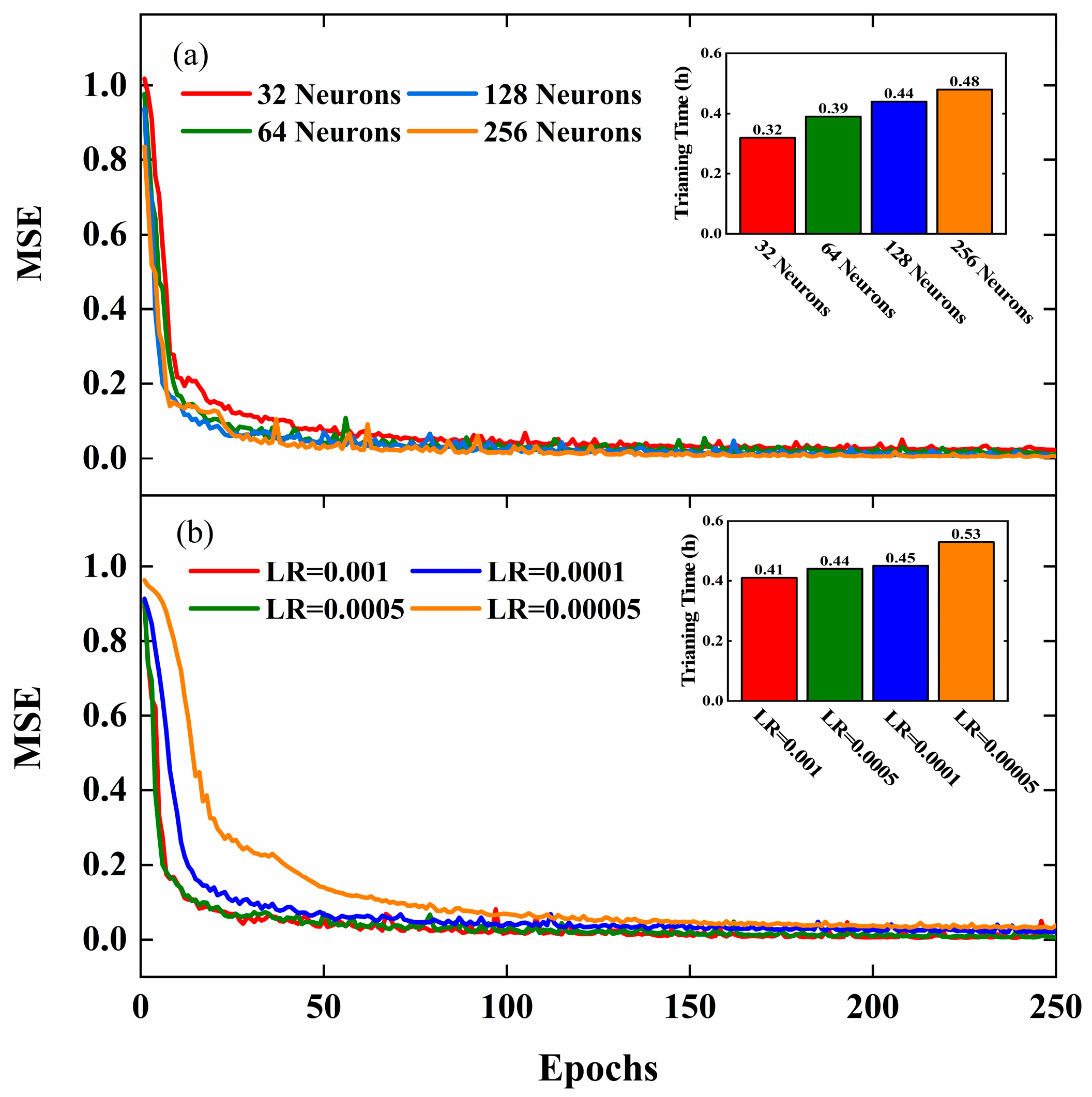
In neural networks, the greater the number of neurons in the hidden layer, the stronger the learning ability and efficiency are, which is obviously beneficial for training complex and nonlinear samples. However, when there are too many neurons in the hidden layer, overfitting may occur. This leads to good results in training but poor identification results in the final output [32]. In this paper, GRU neural networks with 32, 64, 128, and 256 hidden neurons are constructed, and the loss function during training is MSE. The results are shown in Figure 7a, and the upper right corner of the figure is the corresponding training time. The identification precision of the test set is evaluated by MSE, RMSE, MAE, and R2, and the results are shown in Table 5. When the number of hidden neurons increases from 32 to 128, the learning ability and efficiency of the model are improved accordingly. When the number of hidden neurons increases from 128 to 256, the learning ability of the model does not improve significantly, but the learning efficiency decreases significantly. Therefore, considering the learning ability and efficiency, the optimal number of hidden neurons is 128.

3.3.2. Effect of Learning Rate

As an important hyperparameter in deep learning, the learning rate controls the learning progress of the network model and determines whether it is successful or how long it takes to successfully find the global minimum. When the learning rate is too large, the global minimum may be skipped, resulting in nonconvergence of the network. When the learning rate is too low, the network convergence speed is slow and may be trapped in a local optimum [33]. In this paper, GRU neural networks with learning rates of 0.001, 0.0005, 0.0001, and 0.00005 are constructed. The results are shown in Figure 7b, and the evaluation index of the identification results is shown in Table 5. When the learning rate is 0.0005, the convergence speed and identification precision are the highest. Therefore, on the premise of ensuring recognition precision, the optimal learning rate of this model is 0.0005.

4. Conclusions

In this paper, a GRU neural network-based differential settlement of track foundation identification method is proposed. The longitudinal continuous differential settlement distribution curve of track foundations could be successfully identified by the proposed method based on the real-time vibration response of the vehicle–track. The advantage of this method is that the real-time longitudinal continuous track foundation settlement distribution of the whole line can be obtained, which is not realized with other methods in the monitoring of track foundation settlement. The method may provide a useful tool for real-time monitoring of the differential settlement of track foundations. In the study process of this method, two problems are mainly solved: (1) the vehicle–track dynamic response index, which is regular and sensitive to the differential settlement of track foundations, is found; and (2) the feasibility and precision of the GRU neural network to identify the differential settlement of track foundations with sensitive response indexes are verified through numerical simulations, experimental tests, and on-site tests. The conclusions can be summarized as follows:
(1) The vertical acceleration of the vehicle and the wheel–rail contact force are most sensitive to differential settlement of the track foundation, and their change regularity is obvious with the change in the train speed, settlement wavelength, and amplitude. With the increase in settlement amplitude and train speed, the vehicle–track vibration response significantly enhances: the vertical acceleration amplitude of the vehicle increases in both positive and negative directions, and the maximum value of the wheel–rail contact force significantly increases while the minimum value significantly decreases; As the settlement wavelength increases, the vehicle–track vibration response gradually weakens.
(2) The vertical acceleration of the vehicle is an ideal dynamic response index to identify the differential settlement of the track foundation; the wheel–rail contact force is not suitable for identifying the differential settlement of the track foundation because it is sensitive to the changes in stiffness of the vehicle–track elements.
(3) Due to the magnitude of small amplitude settlement being similar to the random unevenness of the track, the GRU neural network model has significantly higher identification precision for large amplitude settlement than for small amplitude settlement.
(4) The change in train speed will increase the complexity of the vehicle–track dynamic response, leading to a decrease in the identification precision of differential settlement of track foundation. In order to improve the identification precision, the train should be kept at a uniform speed when driving the inspection train to collect the vertical acceleration of the train.
(5) To avoid large identification errors of the GRU neural network at the beginning of the time history of the loading process, the input data length could be appropriately increased to include the whole settlement waveform.
(6) According to parameter analyses, the hidden neurons’ quantity and learning rates have a significant impact on the identification precision and training efficiency of the GRU neural network. The optimal hidden neurons quantity of GRU is 128, and the optimal learning rate is 0.0005.
(7) In the study based on engineering-measured data, the identification precision can still be further improved, and higher requirements are put forward for the sample data. In the future, further verification is needed on more rail transit lines.

Author Contributions

Conceptualization, J.J. and H.Z.; Methodology, Y.Z.; Software, L.D.; Formal analysis, H.Z.; Resources, J.J.; Data curation, L.D.; Writing—original draft, L.D.; Writing—review and editing, J.J., Y.Z. and H.Z. All authors have read and agreed to the published version of the manuscript.

Funding

This work is supported by the National Key R&D Program of China under grant No. 2020YFA0711700; the National Natural Science Foundation of China under the grant Nos. 52122801, 51978609, 11925206 and U22A20254; and Zhejiang Provincial Natural Science Foundation of China for Distinguished Young Scholar under grant No. LR20E080003.

Data Availability Statement

Not applicable.

Conflicts of Interest

The authors declare that they have no known competing financial interests or personal relationships that could have appeared to influence the work reported in this paper.

References

  1. Guo, Y.; Zhai, W.; Sun, Y. A mechanical model of vehicle-slab track coupled system with differential subgrade settlement. Struct. Eng. Mech. 2018, 66, 15–25. [Google Scholar]
  2. Guo, Y.; Zhai, W. Long-term prediction of track geometry degradation in high-speed vehicle–ballastless track system due to differential subgrade settlement. Soil Dyn. Earthq. Eng. 2018, 113, 1–11. [Google Scholar] [CrossRef]
  3. Jiang, H.; Li, X.; Xin, G.; Yao, Z.; Zhang, J.; Liang, M. Geometry mapping and additional stresses of ballastless track structure caused by subgrade differential settlement under self-weight loads in high-speed railways. Transp. Geotech. 2019, 18, 103–110. [Google Scholar] [CrossRef]
  4. Cui, X.; Xiao, H. Interface mechanical properties and damage behavior of CRTS II slab track considering differential subgrade settlement. KSCE J. Civ. Eng. 2021, 25, 2036–2045. [Google Scholar] [CrossRef]
  5. Bian, X.; Jiang, H.; Chang, C.; Hu, J.; Chen, Y. Track and ground vibrations generated by high-speed train running on ballastless railway with excitation of vertical track irregularities. Soil Dyn. Earthq. Eng. 2015, 76, 29–43. [Google Scholar] [CrossRef]
  6. Zhang, X.; Burrow, M.; Zhou, S. An investigation of subgrade differential settlement on the dynamic response of the vehicle–track system. Proc. Inst. Mech. Eng. Part F J. Rail Rapid Transit 2016, 230, 1760–1773. [Google Scholar] [CrossRef]
  7. Xu, Q.Y.; Li, B.; Fan, H. Influence of uneven settlement of subgrade on dynamic characteristic of train-Ballastless track on subgrade coupling system. J. Railw. Sci. Eng. 2012, 9, 13–19. [Google Scholar]
  8. Paixao, A.; Fortunato, E.; Calcada, R. The effect of differential settlements on the dynamic response of the train–track system: A numerical study. Eng. Struct. 2015, 88, 216–224. [Google Scholar] [CrossRef]
  9. Qiu, D.; Liang, Q.; Li, Q.; Wu, R. Safety monitoring information system of urban subway. In Proceedings of the 2009 WASE International Conference on Information Engineering, Taiyuan, China, 10–11 July 2009; Volume 2, pp. 426–428. [Google Scholar]
  10. Teskey, W.F. Special survey instrumentation for deformation measurements. J. Surv. Eng. 1988, 114, 2–12. [Google Scholar] [CrossRef]
  11. Abidin, H.Z.; Andreas, H.; Djaja, R.; Darmawan, D.; Gamal, M. Land subsidence characteristics of Jakarta between 1997 and 2005, as estimated using GPS surveys. GPS Solut. 2008, 12, 23–32. [Google Scholar] [CrossRef]
  12. Yin, Z.Z. Application of Hydrostatic leveling system in metro monitoring for construction deep excavation above shield tunnel. Appl. Mech. Mater. 2013, 333–335, 1509–1513. [Google Scholar] [CrossRef]
  13. Stramondo, S.; Bozzano, F.; Marra, F.; Wegmuller, U.; Cinti, F.R.; Moro, M.; Saroli, M. Subsidence induced by urbanisation in the city of Rome detected by advanced InSAR technique and geotechnical investigations. Remote Sens. Environ. 2008, 112, 3160–3172. [Google Scholar] [CrossRef]
  14. Gabriel, A.K.; Goldstein, R.M.; Zebker, H.A. Mapping small elevation changes over large areas: Differential radar interferometry. J. Geophys. Res. Atmos. 1989, 94, 9183–9191. [Google Scholar] [CrossRef]
  15. Wang, X.; Wu, L.; Zhou, Y.; Wang, Y. The long-term settlement deformation automatic monitoring system for the Chinese high-speed railway. Shock Vib. 2015, 2015 Pt 2, 1–12. [Google Scholar] [CrossRef]
  16. Lu, X.; Gong, Y.; Zheng, X.; Du, L.; Wu, Y.; Li, D.; Liu, L.; Yao, Y.; Xiao, S.; Deng, Z.; et al. Field trials of fiber Bragg grating settlement sensors in high-speed railways. In Proceedings of the OFS2012 22nd International Conference on Optical Fiber Sensors, Beijing, China, 14–19 October 2012; Volume 8421, pp. 1767–1770. [Google Scholar]
  17. Zhang, H.; Zhou, Y.; Huang, Z.; Shen, R. Multiparameter Identification of Bridge Cables Using XGBoost Algorithm. J. Bridge Eng. 2023, 28, 04023016. [Google Scholar] [CrossRef]
  18. Zhang, H.; Shen, M.; Zhang, Y.; Chen, Y.; Lü, C. Identification of static loading conditions using piezoelectric sensor arrays. J. Appl. Mech. 2018, 85, 011008. [Google Scholar] [CrossRef]
  19. Xiang, T.; Huang, K.; Zhang, H.; Zhang, Y.; Zhang, Y.; Zhou, Y. Detection of moving load on pavement using piezoelectric sensors. Sensors 2020, 20, 2366. [Google Scholar] [CrossRef]
  20. Zhang, H.; Zhou, Y. AI-based modeling and data-driven identification of moving load on continuous beams. Fundam. Res. 2022, in press. [Google Scholar] [CrossRef]
  21. Zhang, H.; Zhou, Y.; Quan, L. Identification of a moving mass on a beam bridge using piezoelectric sensor arrays. J. Sound Vib. 2021, 491, 115754. [Google Scholar] [CrossRef]
  22. Tian, J.S. Prediction of engineering settlement and deformation based on grey theory model. IOP Conf. Ser. Earth Environ. Sci. 2019, 218, 12079. [Google Scholar] [CrossRef]
  23. Liu, H.B.; Xiang, Y.M.; Wang, H.Z. A multivariable grey model and its application to subgrade settlement prediction. Adv. Mater. Res. 2012, 594–597, 570–573. [Google Scholar] [CrossRef]
  24. Li, X.Y.; Bu, F.J. Prediction of settlement of soft clay foundation in highway using artifical neural networks. Adv. Mater. Res. 2012, 443–444, 15–20. [Google Scholar] [CrossRef]
  25. Zhang, N.; Zhou, A.; Pan, Y.; Shen, S.-L. Measurement and prediction of tunnelling-induced ground settlement in karst region by using expanding deep learning method. Measurement 2021, 183, 109700. [Google Scholar] [CrossRef]
  26. Zhang, R. Application of wavelet neural network in building settlement prediction. E3S Web Conf. 2020, 198, 03014. [Google Scholar] [CrossRef]
  27. Zhu, L.; Huang, T.; Shen, Y.; Zeng, X. Study on tunnel settlement prediction method based on parallel grey neural network model. In Proceedings of the SPIE, International Conference on Intelligent Earth Observing and Applications, Guilin, China, 23–24 October 2015; Volume 9808, pp. 686–692. [Google Scholar]
  28. Liang, B.; Wei, G. Ediction of railway settlement deformation based on improved GM-AR model. J. Phys. Conf. Ser. 2021, 2044, 012154. [Google Scholar] [CrossRef]
  29. Ma, X.L.; Tao, Z.M.; Wang, Y.H.; Yu, H.; Wang, Y. Long short-term memory neural network for traffic speed prediction using remote microwave sensor data. Transp. Res. Part C Emerg. Technol. 2015, 54, 187–197. [Google Scholar] [CrossRef]
  30. Jiang, J.Q.; Dong, B.B.; Ding, Z.; Wei, G.; Liao, J. Dynamic analysis of metro train-monolithic bed track system under tunnel differential settlement. Shock Vib. 2020, 2020, 1–12. [Google Scholar] [CrossRef]
  31. Safarik, J.; Jalowiczor, J.; Gresak, E.; Rozhon, J. Genetic algorithm for automatic tuning of neural network hyperparameters. In Proceedings of the SPIE, Autonomous Systems: Sensors, Vehicles, Security and the Internet of Everything, Orlando, FL, USA, 15–19 April 2018. [Google Scholar]
  32. Madhiarasan, M.; Deepa, S.N. Comparative analysis on hidden neurons estimation in multi layer perceptron neural networks for wind speed forecasting. Artif. Intell. Rev. Int. Sci. Eng. J. 2017, 48, 449–471. [Google Scholar] [CrossRef]
  33. Zhang, S.; Song, Z. An ethnic costumes classification model with optimized learning rate. In Proceedings of the SPIE, Eleventh International Conference on Digital Image Processing (ICDIP 2019), Guangzhou, China, 10–13 May 2019; Volume 11179, pp. 425–431. [Google Scholar]
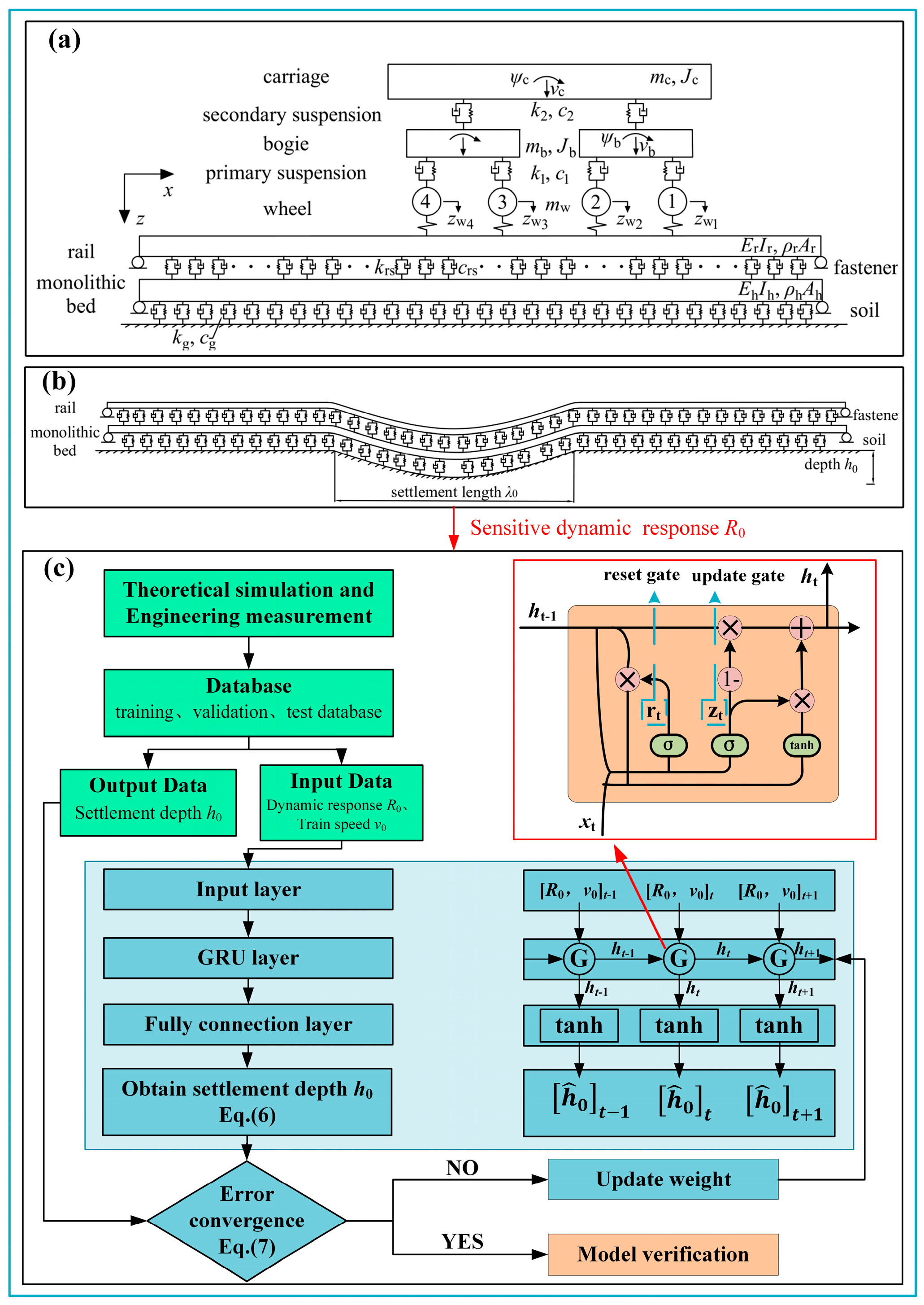
Figure 1. Flow chart of track foundation settlement identification based on the GRU neural network: (a) the train–monolithic bed track model; (b) the differential settlement of track foundation; (c) GRU neural network model.
Remotesensing 15 02378 g001
Figure 2. Vehicle–track dynamic response under a differential settlement of the track foundation: (a) the vertical acceleration of the vehicle with different settlement wavelengths, (i) settlement amplitudes, (ii) and train running speeds (iii); (b) the wheel–rail contact force with different settlement amplitudes (i) and wavelengths (ii).
Remotesensing 15 02378 g002
Figure 3. The coherence function calculation results: (a) the coherence function value between the vertical acceleration of vehicle and the differential settlement of the track foundation; (b) the coherence function value between the wheel–rail contact force and the differential settlement of the track foundation.
Remotesensing 15 02378 g003
Figure 4. (a) Track foundation settlement identification results based on GRU neural network: Complete settlement waveform of single velocity group; (b) the spatial error distribution of the identification results of 20-20-10.
Remotesensing 15 02378 g004
Figure 5. Track foundation settlement identification results based on GRU neural network: (a) Complete settlement waveform of mixing velocity group; (b) 1/2 settlement waveform of mixing velocity group.
Remotesensing 15 02378 g005
Figure 6. (a) Engineering measured data and (b) identification results.
Remotesensing 15 02378 g006
Figure 7. The convergence process and the total time cost of the GRU network training: (a) using different hidden neuron quantities; (b) using different learning rates.
Remotesensing 15 02378 g007
Table 1. Evaluation index for the identification result of the complete settlement waveform of a single velocity group.
Output ConditionInput CombinationnRMSEMAPER2
20-20-10 a c + v 0 −12.9%17.9%0.93751
F w r + v 0 −75.3%98.3%0.54152
a c + F w r + v 0 −66.7%67.9%0.84767
20-100-75 a c + v 0 −2.4%13.8%0.99832
F w r + v 0 −9.0%28.1%0.98203
a c + F w r + v 0 −8.3%24.2%0.98997
Table 2. Evaluation indexes for the identification result of the complete settlement waveform of the mixing velocity group.
20-100-8525-20-2032-60-45
nRMSE−2.7%−15.8%−6.0%
MAPE15.1%22.6%18.9%
R20.997250.925900.99508
Table 3. Evaluation indexes for the identification result of the 1/2 settlement waveform of the mixing velocity group.
20-20-20 (40–180 m)25-80-70 (180–320 m)32-60-30 (40–180 m)
nRMSE−9.9%−8.7%−5.9%
MAPE23.2%9.2%28.5%
R20.976210.993950.99757
Table 4. Evaluation indexes for the identification result of engineering measurement verification.
nRMSEMAPER2
17.3%15.1%0.83134
Table 5. Evaluation Index of Identification Results of Different Hyperparametric Models.
nRMSEMAPER2
32 Neurons−19.3%28.5%0.83569
64 Neurons−17.6%22.4%0.96513
128 Neurons−4.4%15.1%0.99508
256 Neurons−4.1%15.0%0.99729
LR = 0.001−13.9%21.6%0.96423
LR = 0.0005−5.1%14.6%0.99547
LR = 0.0001−9.4%16.3%0.98654
LR = 0.00005−12.7%19.8%0.95715
Disclaimer/Publisher’s Note: The statements, opinions and data contained in all publications are solely those of the individual author(s) and contributor(s) and not of MDPI and/or the editor(s). MDPI and/or the editor(s) disclaim responsibility for any injury to people or property resulting from any ideas, methods, instructions or products referred to in the content.