Estimation of Net Ecosystem Productivity on the Tibetan Plateau Grassland from 1982 to 2018 Based on Random Forest Model

Abstract

The Tibetan Plateau (TP) is one of the most important areas for the study of the carbon budgets of terrestrial ecosystems. However, the estimation of the net ecosystem productivity (NEP) remains uncertain in this region due to its complex topographic properties and climatic conditions. Using CO₂-eddy-covariance-flux data from 1982 to 2018 at 18 sites distributed around the TP grassland, we analyzed the spatial–temporal patterns of the grassland NEP and its driving factors from 1982 to 2018 using a random forest (RF) model. Our results showed that the RF model captured the size of the carbon sink (R² = 0.65, p < 0.05) between the observed and simulated values for the validation samples. During the observation period, the grassland acted as a carbon sink of 26.2 Tg C yr⁻¹ and increased significantly, by 0.4 g C m⁻² yr⁻¹. On a regional scale, the annual NEP gradually increased from the northwest to the southeast, and a similar pattern was also observed in the long-term trends. Furthermore, the moisture conditions, such as the specific humidity and precipitation, were proven to be the main driving factors of the carbon flux in the southeastern areas, while the temperature predominantly controlled the carbon flux in the northwest. Our results emphasize the net carbon sink of the TP and provide a reliable way to upscale NEP from sites.

1. Introduction

Terrestrial ecosystems regulate climates and mitigate global warming by exchanging energy and carbon with the atmosphere [1]. Grassland ecosystems, as crucial components of the terrestrial biosphere, play an important role in the terrestrial carbon cycle [2]. Net ecosystem productivity (NEP) is defined as the difference between net primary production (NPP) and heterotrophic respiration (Rh) [3]. As a direct indicator of carbon sources or sinks, NEP has been widely used to evaluate spatial–temporal patterns of carbon balance [4]. However, the magnitude and distribution of NEP demonstrate large spatial variability across different regions due to environmental and biological factors [5,6]. As a result, considerable uncertainty exists regarding the carbon budget under conditions of global climate change, especially in high-altitude and high-latitude regions, which store large amounts of permafrost soil carbon [7].

During recent decades, many approaches have been developed to estimate and qualify carbon dynamics [8,9,10]. At the site level, the eddy covariance (EC) technique provides high temporal resolution and landscape-scale coverage observations and is thought of as an ideal approach to the capturing of continuous data [11]. These observations are then used to upscale NEP to regional wall-to-wall maps, which are essential for analyzing the spatiotemporal patterns of NEP and its controlling processes [4,12]. Considerable progress has been made in the upscaling of flux observations from towers to regional scales [13,14]. However, site-level measurements only represent several square kilometers around the flux tower. Process-based models combined with satellite-remote-sensing and meteorological data provide a potentially valuable method for NEP upscaling [15]. The CENTURY [16], TEM [17], ORCHIDEE [18], and IBIS models [19] have all been commonly used in the past few years. However, the magnitudes of carbon sinks differed significantly in various model simulations [20]. These models may have included bias due to the neglect of human-disturbance factors and ecosystem management, as well as systematic deviations in their technical aspects and the considerable differences between their parameters [10,21]. To achieve a more comprehensive and accurate understanding of carbon dynamics over larger areas, machine learning (ML) techniques are receiving increasing attention from researchers dealing with different issues in ecological fields [22,23]. As a data-oriented approach, machine learning performs with a high degree of accuracy and has proven to be an improvement on previous approaches [24,25,26]. For this reason, ML algorithms, such as random forest (RF), artificial neural networks (ANNs) and support vector regression (SVR), are widely used in the estimation of carbon budgets around the world [27,28,29]. In particular, the RF algorithm makes no distributional assumptions about predictor variables and is not sensitive to noise or over-fitting; therefore, it can model complex interactions with fewer parameters in comparison with other machine-learning algorithms [30,31]. The simulations of net primary productivity (NPP), gross primary productivity (GPP), and net ecosystem exchange (NEE) all produced relatively reliable results [26,32,33]. However, the studies referred to above lacked region-specific analyses and were limited by the number and distribution of flux towers.

The Tibetan Plateau (TP) is considered “the third pole,” and it has experienced significant climate warming over the past few decades, at an even faster rate than the mean trend in China [34]. As the dominant vegetation type, alpine grassland in the TP is sensitive to climate change and has a strong impact on the terrestrial carbon cycle [18]. The unique topography and climatic features of the TP grassland also make it an ideal region for investigating the carbon balance and its spatial variation [35]. Therefore, it is crucial to accurately monitor and estimate the carbon budget in grassland ecosystems in future climate scenarios and to develop an understanding of the feedback between the terrestrial biosphere and the atmosphere in response to climate change [36,37]. In this study, we developed a random forest (RF) model based on NEP data from 18 grassland-eddy-covariance sites, combined with meteorological data and remote-sensing data covering the TP grassland from 1982 to 2018. The goals of this study were to: (1) extrapolate the NEP model to the whole grassland at a spatial resolution of 0.1° × 0.1° for each 8-day period; (2) estimate the size of the carbon sink; and (3) explore the spatial-temporal patterns of the carbon sink and their driving mechanisms.

2. Materials and Methods

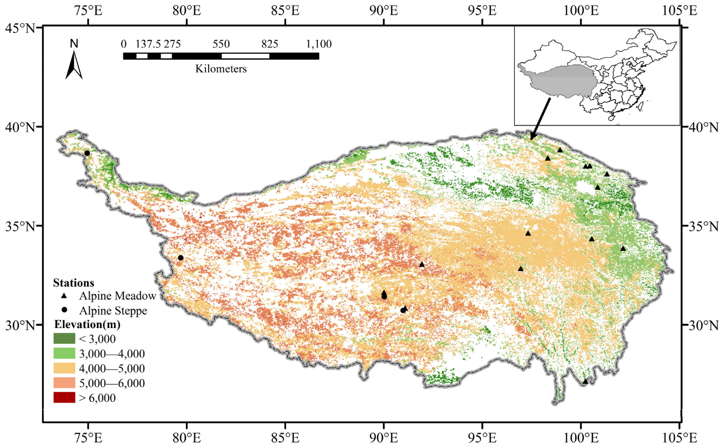
2.1. Study Area

The Tibetan Plateau (TP), known as “the third ladder of China”, ranges from 26°00′12″ to 39°46′50″ in latitude, and 73°18′52″ to 104°46′59″ in longitude [38], with an average elevation of more than 4000 m above sea level (Figure 1). The annual mean temperature ranges from −3.1 °C to 4.4 °C and the annual average precipitation ranges from 350 mm to 700 mm. The grassland across the TP covers about 1.25 million km² and is dominated by alpine meadows and alpine steppes, which account for about 27% and 34% of the whole plateau, respectively [39]. The distribution map of grassland was derived from https://www.resdc.cn/DOI, accessed on 20 April 2022 (reprinted with permission from Ref. [40]. 2018, Xu X). The TP is one of the most unique physico-geographical regions on Earth; thus, it plays an important role in the modulation of regional patterns and mechanisms under conditions of global climate change.

2.2. Data Collection

2.2.1. Eddy-Covariance-Flux Data

We obtained two types of NEP data from 18 grassland-eddy-covariance sites within the study area. Specifically, the data from 16 stations were research-based, and the data from 2 stations were obtained by contacting the original researchers (

Table 1. Site descriptions and technical details of eddy-covariance observations.

Station	Latitude (°N)	Longitude (°E)	Altitude (m)	Period	Ecosystem	NEP (g C m−2 yr−1)	Reference
Ali	4270	33.38	79.7	2010–2011	Steppe	206.9	[41]
Arou	3033	38.03	100.45	2015	Meadow	31.7	[41]
Batang	4003	32.85	96.95	2017–2018	Meadow	429.6	[41]
Bange	4700	31.42	90.03	2014–2015	Steppe	314.0	[41]
Dashalong	3739	38.84	98.94	2015	Meadow	−21.8	[41]
Dangxiong	4333	30.85	91.08	2004–2011	Meadow	−35.7	[42]
Guoluo	3980	34.35	100.55	2010–2012	Meadow	25.3	[41]
Haibei	3250	37.60	101.33	2002–2004	Meadow	120.9	[41]
Haiyan	3140	36.95	100.85	2010.7–2011.7	Meadow	66.9	[41]
Maoniuping	3560	27.17	100.23	2012–2015	Meadow	161.8	[41]
Maduo	4316	34.63	97.32	2014	Meadow	164.8	[41]
Muztag	3668	38.66	74.95	2016	Steppe	60.2	[41]
NamCo	4730	30.72	90.98	2008–2009	Steppe	17.1	[41]
Naqu	4598	31.64	90.01	2012–2018	Meadow	3.0	[43]
Shule	3885	38.42	98.32	2009–2011	Meadow	43.4	[41]
Tanggula	5133	33.07	91.93	2007	Meadow	−75.8	[41]
Yakou	4148	38.01	100.24	2015	Meadow	151.6	[41]
Zoige	3430	33.89	102.14	2010	Meadow	156.4	[41]

). The eddy-covariance sites covered 2 grassland types in the study area, namely alpine meadows (14 sites) and alpine steppes (4 sites), which were primarily located in the central and southeast areas of the TP (Figure 1). All the sites were at altitudes ranging from 3033 to 5133 m, and the time spans of these flux sites varied from 1 to 7 years, providing 44 years of site data. The data presented can reflect the basic characteristics of the TP grassland. The daily fluxes were recalculated at 8-day intervals by summing every 8 days to match the period of remote-sensing data.

2.2.2. Meteorological Data

Daily meteorological data in this paper include precipitation rate (PREC, mm/h), specific humidity (SHUM, kg/kg), downward shortwave radiation (SRAD, W/m²), temperature (TEMP, °C), and wind speed (WIND, m/s). The meteorological factors that we chose showed a high correlation with carbon fluxes in previous studies [9]. The data were collected from the China Meteorological Forcing Dataset (CMFD) for the period of 1982–2018 with a resolution of 0.1° × 0.1°. In particular, we multiplied precipitation-rate data by 24 to convert them to daily precipitation, and subtracted temperature data by 273.15, converting Calvin to Celsius. All the data were calculated at 8-day intervals to match the period of remote-sensing data.

2.2.3. Remote-Sensing Data

The 8-day leaf-area index (LAI) and fraction of absorbed photosynthetically active radiation (FAPAR) data were extracted from http://www.glass.umd.edu, accessed on 20 January 2020. The LAI and FAPAR are important indicators used to characterize vegetation growth and photosynthesis [44]. We downloaded the data at a resolution of 0.05° × 0.05° from 1982 to 2018 via the advanced very high resolution radiometer (AVHRR) dataset. We used the “Resample” tool in ArcGIS 10.2 to resample the remote-sensing data to a resolution of 0.1° × 0.1° using the “nearest neighbor interpolation” method to match the meteorological data.

2.3. Random Forest Model

Random forest (RF) is a typical ensemble and flexible method in machine learning (ML), and it is an effective tool for estimating carbon flux. Random samples are formed by selecting random variables from the training data, and all the explanatory variables exert an impact on model-simulation results [45]. Generally, RF is an ensemble of classification or regression trees that are calculated on random subsets of data. Although the working process of the model is mostly in a black box and is often difficult to fully understand, RF has higher accuracy than other traditional models [23,46]. Two key parameters need to be defined in the RF model: ntree, the number of bootstrap samples; and mtry, the number of different predictors tested at each node [47]. In this study, we used 7 environmental variables, including 5 meteorological properties (PREC, SHUM, SRAD, TEMP, and WIND) and 2 remote-sensing properties (LAI and FAPAR) as explanatory variables and NEP as the target variable (Figure 2). After converting the daily flux data to 8 days, we obtained a total of 1986 samples, 80% of which were used for training, while the remaining 20% were used for verification. We used 1500 “ntree” and 3 “mtry” to develop the best-fitting model. Finally, we imported the raster data of all variables into the model to estimate the regional NEP. The RF model was run with Python 3.7.

2.4. Data Analysis

2.4.1. Theil-Sen Median Trend Analysis of the Annual NEP

Theil–Sen median trend analysis, also known as Sen slope estimation, is a non-parametric method for estimating the slope of a trend in N pairs of data samples [48], expressed as follows:

$$\mathsf{\beta }=\mathrm{m}\mathrm{e}\mathrm{d}\mathrm{i}\mathrm{a}\mathrm{n}\left(\frac{{\mathrm{y}}_{\mathrm{j}}-{\mathrm{y}}_{\mathrm{i}}}{\mathrm{j}-\mathrm{i}}\right),\forall \mathrm{i}<\mathrm{j}$$

where refers to the Theil–Sen median and represents the variable (NEP) value of years i and j. If >0, the variable presents an increasing trend; otherwise, the variable displays a decreasing trend.

2.4.2. Partial Correlation Analysis between NEP and Climate Factors

Partial correlation analysis means that when a variable is correlated with multiple variables at the same time, only the correlation between that variable and one of the other variables is analyzed, and the influence of these other variables is eliminated. For example, if y is correlated with x₁, x₂, and x₃, the partial correlation coefficient (R_p) between y and x₁ is defined as:

$${\mathrm{r}}_{\mathrm{y}{\mathrm{x}}_1,{\mathrm{x}}_2}=\frac{{\mathrm{r}}_{\mathrm{y}{\mathrm{x}}_1}-{\mathrm{r}}_{\mathrm{y}{\mathrm{x}}_2}{\mathrm{r}}_{{\mathrm{x}}_1{\mathrm{x}}_2}}{\sqrt{(1-{\mathrm{r}}_{\mathrm{y}{\mathrm{x}}_2}^2)(1-{\mathrm{r}}_{{\mathrm{x}}_1{\mathrm{x}}_2}^2)}}$$

$${\mathrm{r}}_{\mathrm{y}{\mathrm{x}}_1,{\mathrm{x}}_2{\mathrm{x}}_3}=\frac{{\mathrm{r}}_{\mathrm{y}{\mathrm{x}}_1,{\mathrm{x}}_2}-{\mathrm{r}}_{\mathrm{y}{\mathrm{x}}_3,{\mathrm{x}}_2}{\mathrm{r}}_{{\mathrm{x}}_1{\mathrm{x}}_3,{\mathrm{x}}_2}}{\sqrt{(1-{\mathrm{r}}_{\mathrm{y}{\mathrm{x}}_3,{\mathrm{x}}_2}^2)(1-{\mathrm{r}}_{{\mathrm{x}}_1{\mathrm{x}}_3,{\mathrm{x}}_2}^2)}}$$

where ${\mathrm{r}}_{\mathrm{y}{\mathrm{x}}_1,{\mathrm{x}}_2}$ is the partial correlation coefficient between y and x₁ when the influence of x₂ is removed, and ${\mathrm{r}}_{\mathrm{y}{\mathrm{x}}_1,{\mathrm{x}}_2{\mathrm{x}}_3}$ is the partial correlation coefficient between y and x₁ when the influence of x₂ and x₃ is removed. The remainder can be performed in the same manner. This approach can be used to represent the degree of statistical correlation between the two variables, and its value is between the intervals (−1, 1).

3. Results

3.1. Performance of Estimation of NEP Using the Random Forest Model

We evaluated the performance of the RF model and used the R² coefficient and mean square error (MSE) to quantify it. We constructed a model that accurately reflected the observed data, with an R² of 0.65 and an MSE of 3.56 g C m² 8 d⁻¹ between the observed and simulated values for the validation samples (Figure 3a). We also calculated the importance of different input features using the random forest classifier. The values of the importance of the PREC, SHUM, SRAD, TEMP, WIND, LAI, and FAPAR were 10.1%, 48.4%, 11.0%, 41.8%, 22.3%, 22.3%, and 20.7%, respectively (Figure 3b). This result demonstrated not only the good predictive ability of the RF model for flux data, but also the considerable role of humidity and temperature in alpine ecosystems.

3.2. Spatial and Temporal Patterns of NEP

Our results showed that the TP grassland acted as a weak carbon sink, with a mean annual NEP of 21.0 $\pm$ 7.2 g C m² yr⁻¹, which is equivalent to 26.2 $\pm$ 9.0 T g C yr⁻¹, from 1982 to 2018. The larger carbon sinks mainly appeared in the western region, while the larger carbon sources appeared in the northwestern region. During the research period, the mean annual NEP exhibited a significantly increasing trend of 0.4 g C m⁻² yr⁻¹ (p < 0.05) (Figure 4). The minimum and maximum values were 7.7 g C m² yr⁻¹ in 1982 and 37.3 g C m² yr⁻¹ in 1998, respectively. There was a large spatial variability in the mean annual NEP over the TP grassland, with a generally increasing gradient from the northwest to the southeast (Figure 5a). Despite the increasing trend in the NEP from 1982 to 2018, it displayed strong geographical heterogeneity across the TP grassland (Figure 5b). Most of the areas (77.0%) in the region experienced an increasing trend in NEP during the period of 1982–2018, and 55.7% of them reached a significant level (p < 0.05), especially in the southwest and east of Qinghai province, near the “Sanjiangyuan” region. In contrast, only 23.0% of the pixels experienced a decreasing trend in NEP, especially in the northwestern region (p < 0.05).

In addition to horizontal patterns, the NEP also exhibited vertical patterns across the TP grassland. Figure 6 shows the average and standard deviation (SD) of the NEP and its trends for every 200 m elevation bin from 1982 to 2018. The mean annual NEP displayed a decreasing trend with increasing elevation (R² = 0.79, p < 0.05) and tended to be constant above 2000 m (Figure 6a). When the elevation was below 5000 m, the mean annual NEP showed a positive value, indicating carbon sinks at relatively low elevations. The trends of the NEP were positive at all the elevation bins, but the value gradually decreased with increasing elevation (R² = 0.57, p < 0.05). This lower trend at relatively high elevations implied that the NEP became more stable over time at higher elevations.

3.3. Driving Factors of NEP

We performed a partial correlation analysis of the NEP and climate factors to explore the main drivers of the NEP over the TP grassland from 1982 to 2018 (Figure 7). The partial correlation coefficient (R_p) between the annual NEP and the PREC was positive in 68.0% of the region and significant in 15.6% of the pixels, with higher values in the southeast (Figure 7a). The variations in annual NEP over the TP were primarily controlled by the SHUM, with the R_p between the two being positive in almost all of the study area (82.7%) and significant in 47.8% of the pixels, suggesting that higher levels of moisture increased the carbon-sink capacity (Figure 7b). With respect to the TEMP, the correlation between the two was positive for 77.2% of the pixels in the northwestern TP and significant for 31.9% of the pixels (Figure 7d). Nevertheless, the SRAD and WIND had little impact on the NEP. The proportions of positive R_p values between them were 48.3% and 48.5%, respectively, and only 12.3% and 13.5% of them reached a significant level (Figure 7c,e).

We further defined the factor with the largest absolute value of R_p as the driving factor for each pixel and assigned them different colors (Figure 7f). The mean annual NEP over the TP grassland was primarily controlled by the SHUM (44.7%). The following factors were TEMP and PREC, which controlled 28.2% and 11.3% of the study area, respectively. The moisture factors (SHUM and PREC) controlled most of the study area (56.1%), and were mainly located in the southeastern region, while the northwest of the TP and the southern part of Qinghai province were mainly controlled by the heat factor (TEMP), accounting for 28.2% of the study area. The remaining 15.8% was dominated by the SRAD (7.8%) and WIND (8.0%). The results indicated that the SHUM, PREC, and TEMP mainly regulated the annual NEP over the TP grassland, and that the SHUM was the most important. Additionally, the carbon fluxes in different regions had different responses to hydrothermal factors.

4. Discussion

4.1. Driving Factors of Grassland Carbon Sink across the TP

Hydrothermal conditions are important factors regulating the terrestrial carbon cycle because they influence plant distribution and productivity [9]; however, the driving mechanisms of carbon fluxes in various regions are different [49,50]. We found an opposite pattern of NEP controlled by moisture or temperature. In total, 44.7% of the area was primarily controlled by the SHUM, which was distributed in the southeastern and northeastern regions, where alpine meadows constituted the main vegetation type. These results confirmed the findings of several previous studies, which reported that water availability regulates the carbon flux in alpine meadows by affecting soil moisture, which is essential for vegetation growth and physiological processes [51,52]. In warmer regions, photosynthesis reaches saturation, and the demand for evaporation increases [53]. Additionally, increases in moisture may compensate for warming-induced droughts in these areas, further affecting carbon exchange. By contrast, the carbon flux showed a different response to the temperature. The temperature had negative effects on the NEP in the southeast and controlled only 28.2% of the pixels in the northwestern region. Rising temperatures can stimulate plant growth due to the alleviation of temperature limitations in high-elevation regions [54,55]. On the other hand, higher temperatures may have a negative impact on carbon sinks by enhancing ecosystem respiration and decreasing soil moisture, especially in moist areas [56]. This result reflects the weak response of the NEP to temperature at the regional scale.

However, several studies pointed out that the TP grassland was primarily affected by temperature based on a short-term site scale, which was inconsistent with our conclusion [57,58]. One possible reason for this difference is that the effect of the meteorological factors on the NEP was influenced by the time scale. For example, the effect of the temperature probably diminished over time because the equal promotional effect of temperature on both NPP and Rh may lead to insignificant changes in the NEP [59]. Furthermore, the size and spatial patterns of NEP are not merely determined by a single physiological process, but are the joint result of photosynthesis and respiration in response to environmental changes [59,60]. Therefore, the effects of environmental factors on the TP grassland might be inadequate, according to site-scale studies.

4.2. The Size of Carbon Sink over the TP

Our results indicated that the grassland across the TP exhibited a net carbon sink of 26.2 Tg C yr⁻¹ and significantly increased by 0.4 g C m⁻² yr⁻¹ from 1982 to 2018. We reported a net carbon sink across the entire TP. However, the NEP was negative in the southeast of the TP, indicating a net carbon source in these areas. The carbon source, or sink, is mainly controlled by two important components: gross primary productivity (GPP) and ecosystem respiration (ER), which is also affected by temperature and precipitation [9]. In hot and arid regions, the promotional effect of temperature on ER is more significant than on GPP, resulting in CO₂ losses exceeding CO₂ uptake, especially in non-growing seasons [61].

Compared with alpine steppes, the annual NEP of alpine meadows had a more significant increasing trend (Figure 8a), which was consistent with other studies [62,63]. This was probably because of the higher soil-carbon contents in the meadows, which stored 2–3 times more carbon than the alpine steppes. In addition, the alpine meadows had greater vegetation coverage and species diversity due to the adequate supply of water and relatively high temperatures [64,65]. The positive effects of temperature and CO₂ on vegetation are more pronounced in locations with appropriate water availability. Therefore, alpine meadows are more likely to have stronger carbon sinks under conditions of climate change. We also found that the carbon sinks were significantly greater at low latitudes than at middle latitudes (Figure 8b), which was determined by the distribution patterns of the latitude-dependent climate factors, especially temperature and precipitation [5,41]. However, at low latitudes, there was no significant difference between the carbon-sequestration capacities of the alpine meadows and the alpine steppes (Figure 8c). Because the region is mainly controlled by specific humidity, differences in temperature between different latitudes do not cause significant changes in the carbon sink in the alpine meadows.

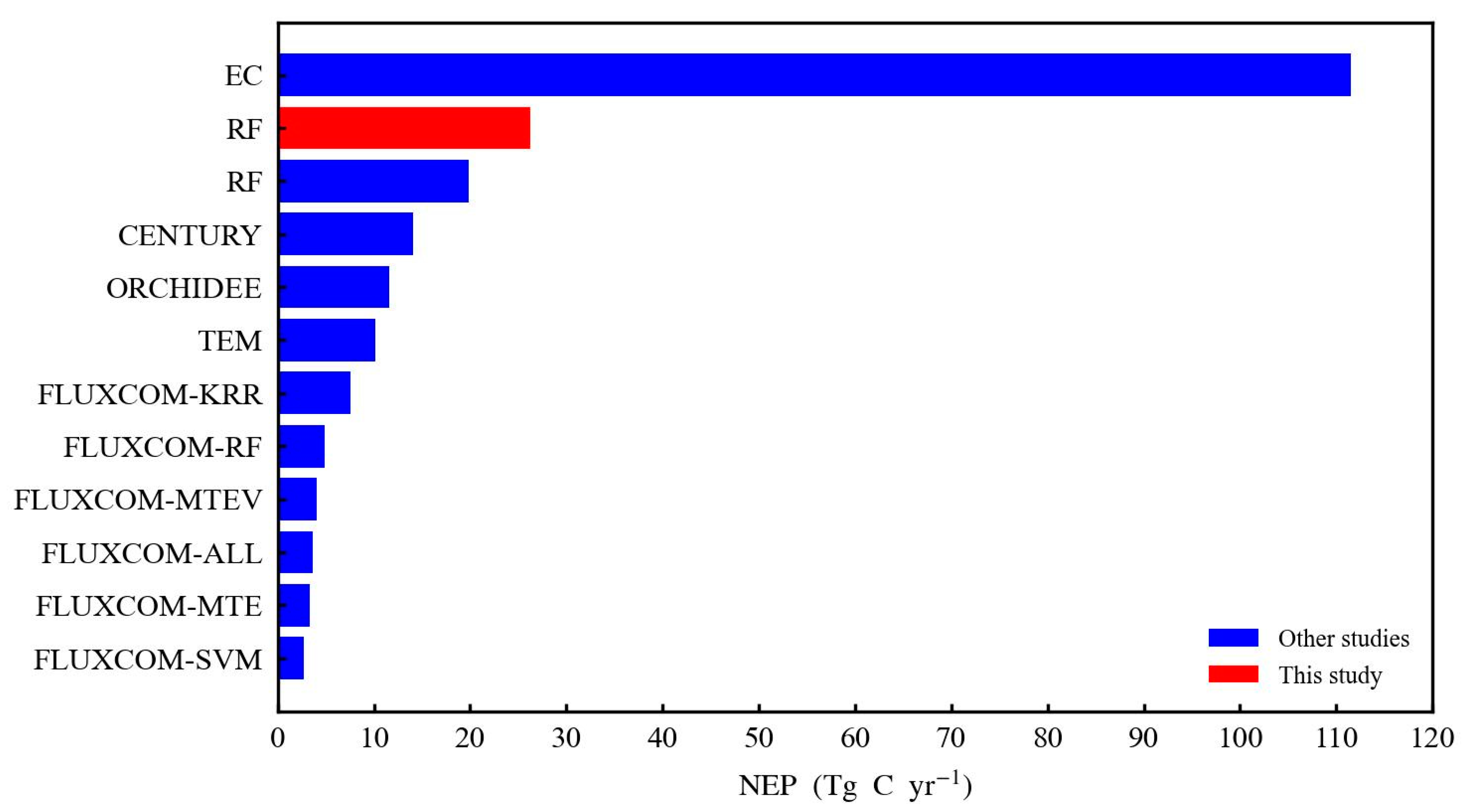
4.3. Comparison with Other Studies

The mapping of the NEP on a large scale based on site measurements is the basis for the quantification of regional carbon budgets. There are two main approaches to this mapping process. One is the site-level-extrapolation approach with direct spatial expansion through flux-tower observations. The other is the model-simulation approach with ecosystem-process models and ML algorithms [67]. To understand the carbon budget in the TP grassland, we compared the mean annual NEP in this study with that in other studies using different approaches. The size of the carbon sink in our study was significantly lower than the site-level results, but slightly higher than those of the modeling studies (Figure 9).

The TP grassland was estimated as having a strong carbon sink of 112.8 Tg C yr⁻¹ based on eddy-covariance observations [41], which was much larger than our results suggested. The estimated NEP throughout the whole region was overestimated when represented only as the average of selected sites. This may have been due to the horizontal representativeness errors in the surrounding area, which were not negligible [68]. Additionally, CO₂-eddy-covariance-flux observations can be easily affected by meteorological conditions, which lead to systematic errors [69,70]. Therefore, it is inaccurate to extrapolate the NEP from field observations using the average values of sites [71].

Process-based models can upscale observed data to a regional scale and quantitatively describe the contribution of different driving factors to changes in carbon storage [72]. Nevertheless, the results of these simulations were largely inconclusive. For example, using the CENTURY model, Lin et al. estimated that the grassland carbon sink of the TP was 14.1 Tg C yr⁻¹ from 1981 to 2010 [16]. Yan et al. estimated that alpine grasslands sequestered carbon at 10.1 Tg C yr⁻¹ from 1961 to 2010, using the TEM model [17]. Based on the ORCHIDEE model, however, Piao et al. suggested that the TP grassland acted as a carbon sink of 11.5 Tg C yr⁻¹ [18]. This inconsistency was probably due to the different parameters and variables used as inputs in the models, as well as the neglect of critical ecosystem processes [73,74].

A recent study simulated a carbon sink of 19.9 Tg C yr⁻¹ with a RF model [28]. The data-oriented products of carbon fluxes in FLUXCOM, driven by nine machine-learning methods and five meteorological forcing datasets, estimated a relatively weak carbon sink of between 2.7 and 7.5 Tg C yr⁻¹ in the TP grassland [29]. The machine-learning models described above are all based on FLUXNET; however, great uncertainty may arise when estimating the NEP in the TP because only four sites in FLUXNET are located there.

In summary, although the size of our estimated carbon sink differed from that in some previous works (Figure 9), the RF model is also considered as a reasonable and suitable method for NEP up-scaling from site measurements to the regional scale in the TP, primarily for the following four reasons. First, our results were close to the modeling-simulation results in other studies and showed good performance in terms of the observation values [16,17,18]. Second, as a machine-learning algorithm, the RF model selected the optimal output from a number of regression trees to capture the characteristics of the data, which effectively improved the accuracy of the flux data [45,73,74]. Third, by extracting multivariate functional relationships between observation data and explanatory variables, the RF model can not only integrate data from different sources but also simplify complex processes and solve nonlinear problems in ecosystems [72]. Fourth, we collected data from 18 grassland-flux stations, which covered almost all the grassland in the TP, to improve the spatial representation of our results.

4.4. Uncertainty and Limitations

In this study, we presented an approach to the estimation of the NEP over the TP grassland using the RF model. This model performed well for the flux data and effectively avoided the calculation of complex parameters and ecological processes; however, there are still several uncertainties and limitations that need to be mentioned. The uncertainties resulted from the explanatory variables, due to the impact of clouds on the remote-sensing data and product-specific biases in the gridded meteorological datasets [46]. The limitations can be summarized in two points, as follows. First, although the selected flux stations covered the major types of grassland, they were still not sufficiently representative of the entirety of the TP, since most of them were located in the southeast TP (Figure 1), limiting the representativeness of the NEP values. Second, beyond the seven variables in this study, there are other important environmental factors that we did not consider, such as land-use change, soil moisture, and nitrogen deposition [25,75].

5. Conclusions

In this study, we combined explanation variables and NEP data from 18 flux sites involving a variety of grassland types to develop a predictive NEP model using a random forest approach. Our study demonstrated that the TP grassland acted as a carbon sink of 26.2 Tg C yr⁻¹, ranging from 7.7 Tg C yr⁻¹ in 1982 to 37.3 Tg C yr⁻¹ in 1998. This value is similar to the model simulation and further verifies the accuracy of our approach. Regarding the spatial patterns, the mean annual and interannual variability trends of the NEP both gradually increased from the northwest to the southeast. We also concluded that hydrothermal factors mainly regulated the carbon sink over the TP grassland, because 44.7% of the TP grassland was controlled by humidity, and 28.2% of this total was more susceptible to temperature. On a regional scale, humidity and precipitation played dominant roles in the regulation of the southeastern areas, while temperature mainly controlled the northwestern areas. The results of this paper provide data and methodological support for the study of carbon cycling over alpine grasslands. The findings help us to better understand the spatial patterns of carbon fluxes in alpine-grassland ecosystems, as well as supporting the construction of ecologically functional areas and ecological service areas under conditions of climate change.

References

1. Ahlstrom, A.; Raupach, M.R.; Schurgers, G.; Smith, B.; Arneth, A.; Jung, M.; Reichstein, M.; Canadell, J.G.; Friedlingstein, P.; Jain, A.K. The dominant role of semi-arid ecosystems in the trend and variability of the land CO2 sink. Science 2015, 348, 895–899. [Google Scholar] [CrossRef]
2. Scurlock, J.M.O.; Hall, D.O. The global carbon sink: A grassland perspective. Glob. Change Biol. 1998, 4, 229–233. [Google Scholar] [CrossRef]
3. Smith, P.; Lanigan, G.; Kutsch, W.L.; Buchmann, N.; Eugster, W.; Aubinet, M.; Ceschia, E.; Béziat, P.; Yeluripati, J.B.; Osborne, B.; et al. Measurements necessary for assessing the net ecosystem carbon budget of croplands. Agric. Ecosyst. Environ. 2010, 139, 302–315. [Google Scholar] [CrossRef]
4. Xiao, J.; Zhuang, Q.; Law, B.E.; Baldocchi, D.D.; Chen, J.; Richardson, A.D.; Melillo, J.M.; Davis, K.J.; Hollinger, D.Y.; Wharton, S.; et al. Assessing net ecosystem carbon exchange of U.S. terrestrial ecosystems by integrating eddy covariance flux measurements and satellite observations. Agric. For. Meteorol. 2011, 151, 60–69. [Google Scholar] [CrossRef]
5. Wagle, P.; Xiao, X.; Scott, R.L.; Kolb, T.E.; Cook, D.R.; Brunsell, N.; Baldocchi, D.D.; Basara, J.; Matamala, R.; Zhou, Y. Biophysical controls on carbon and water vapor fluxes across a grassland climatic gradient in the United States. Agric. For. Meteorol. 2015, 214–215, 293–305. [Google Scholar] [CrossRef]
6. Fu, Y.; Zheng, Z.; Yu, G.; Hu, Z.; Sun, X.; Shi, P.; Wang, Y.; Zhao, X. Environmental influences on carbon dioxide fluxes over three grassland ecosystems in China. Biogeosciences 2009, 6, 2879–2893. [Google Scholar] [CrossRef]
7. Obu, J.; Westermann, S.; Bartsch, A.; Berdnikov, N.; Christiansen, H.H.; Dashtseren, A.; Delaloye, R.; Elberling, B.; Etzelmüller, B.; Kholodov, A. Northern Hemisphere permafrost map based on TTOP modelling for 2000–2016 at 1 km2 scale. Earth-Sci. Rev. 2019, 193, 299–316. [Google Scholar] [CrossRef]
8. Scottdenning, A.; Randall, D.A.; Jamescollatz, G.; Sellers, P.J. Simulations of terrestrial carbon metabolism and atmospheric CO2 in a general circulation model. Part 2: Simulated CO2 concentrations. Tellus 2010, 48, 543–567. [Google Scholar]
9. Yu, G.; Zhu, X.; Fu, Y.; He, H.; Wang, Q.; Wen, X. Spatial patterns and climate drivers of carbon fluxes in terrestrial ecosystems of China. Glob. Change Biol. 2013, 3, 798–810. [Google Scholar] [CrossRef]
10. Piao, S.; He, Y.; Wang, X.; Chen, F. Estimation of China’s terrestrial ecosystem carbon sink: Methods, progress and prospects. Sci. China, Ser. D Earth Sci. 2022, 65, 641–651. [Google Scholar] [CrossRef]
11. Dragoni, D.; Schmid, H.P.; Grimmond, C.S.B.; Loescher, H.W. Uncertainty of annual net ecosystem productivity estimated using eddy covariance flux measurements. J. Geophys. Res. Biogeosci. 2007, 112, D17102. [Google Scholar] [CrossRef]
12. Baldocchi, D.; Falge, E.; Gu, L.; Olson, R.; Hollinger, D.; Running, S. FLUXNET: A new tool to study the temporal and spatial variability of ecosystem-scale carbon dioxide, water vapor, and energy flux densities. Bull. Am. Meteorol. Soc. 2001, 82, 2415–2434. [Google Scholar] [CrossRef]
13. Wang, Y.; Xiao, J.; Ma, Y.; Luo, Y.; Hu, Z.; Li, F.; Li, Y.; Gu, L.; Li, Z.; Yuan, L. Carbon fluxes and environmental controls across different alpine grassland types on the Tibetan Plateau. Agric. For. Meteorol. 2021, 311, 108694. [Google Scholar] [CrossRef]
14. Sun, S.; Che, T.; Li, H.; Wang, T.; Ma, C.; Liu, B.; Wu, Y.; Song, Z. Water and carbon dioxide exchange of an alpine meadow ecosystem in the northeastern Tibetan Plateau is energy-limited. Agric. For. Meteorol. 2019, 275, 283–295. [Google Scholar] [CrossRef]
15. Friedlingstein, P.; O′Sullivan, M.; Jones, M.W.; Andrew, R.M.; Gregor, L.; Hauck, J.; Le Quéré, C.; Luijkx, I.T.; Olsen, A.; Peters, G.P.; et al. Global Carbon Budget 2022. Earth Syst. Sci. Data 2022, 14, 4811–4900. [Google Scholar] [CrossRef]
16. Lin, X.; Han, P.; Zhang, W.; Wang, G. Sensitivity of alpine grassland carbon balance to interannual variability in climate and atmospheric CO 2 on the Tibetan Plateau during the last century. Glob. Planet. Change 2017, 154, 23–32. [Google Scholar] [CrossRef]
17. Yan, L.; Zhou, G.; Wang, Y.; Hu, T.; Sui, X. The spatial and temporal dynamics of carbon budget in the alpine grasslands on the Qinghai-Tibetan Plateau using the Terrestrial Ecosystem Model. J. Cleaner Prod. 2015, 107, 195–201. [Google Scholar] [CrossRef]
18. Piao, S.; Tan, K.; Nan, H.; Ciais, P.; Fang, J.; Wang, T.; Vuichard, N.; Zhu, B. Impacts of climate and CO2 changes on the vegetation growth and carbon balance of Qinghai–Tibetan grasslands over the past five decades. Glob. Planet. Change 2012, 98–99, 73–80. [Google Scholar] [CrossRef]
19. Wu, T.; Ma, W.; Wu, X.; Li, R.; Qiao, Y.; Li, X.; Yue, G.; Zhu, X.; Ni, J. Weakening of carbon sink on the Qinghai–Tibet Plateau. Geoderma 2022, 412, 115707. [Google Scholar] [CrossRef]
20. Xu, L.; Yu, G.; He, N.; Wang, Q.; Ge, J. Carbon storage in China’s terrestrial ecosystems: A synthesis. Sci. Rep. 2018, 8, 1–13. [Google Scholar] [CrossRef]
21. Yu, G.; Wen, X.; Sun, X.; Tanner, B.D.; Lee, X.; Chen, J. Overview of ChinaFLUX and evaluation of its eddy covariance measurement. Agric. For. Meteorol. 2006, 137, 125–137. [Google Scholar] [CrossRef]
22. Kim, Y.; Johnson, M.S.; Knox, S.H.; Black, T.A.; Dalmagro, H.J.; Kang, M.; Kim, J.; Baldocchi, D. Gap-filling approaches for eddy covariance methane fluxes: A comparison of three machine learning algorithms and a traditional method with principal component analysis. Glob. Change Biol. 2020, 26, 1499–1518. [Google Scholar] [CrossRef] [PubMed]
23. Gao, X.; Dong, S.; Li, S.; Xu, Y.; Liu, S.; Zhao, H.; Yeomans, J.; Li, Y.; Shen, H.; Wu, S. Using the random forest model and validated MODIS with the field spectrometer measurement promote the accuracy of estimating aboveground biomass and coverage of alpine grasslands on the Qinghai-Tibetan Plateau. Ecol. Indic. 2020, 112, 106114. [Google Scholar] [CrossRef]
24. Cai, J.; Xu, K.; Zhu, Y.; Hu, F.; Li, L. Prediction and analysis of net ecosystem carbon exchange based on gradient boosting regression and random forest. Appl. Energy 2020, 262, 114566. [Google Scholar] [CrossRef]
25. Zhou, Q.; Fellows, A.; Flerchinger, G.N.; Flores, A.N. Examining Interactions Between and Among Predictors of Net Ecosystem Exchange: A Machine Learning Approach in a Semi-arid Landscape. Sci. Rep. 2019, 9, 2222. [Google Scholar] [CrossRef]
26. Chen, Y.; Shen, W.; Gao, S.; Zhang, K.; Huang, N. Estimating deciduous broadleaf forest gross primary productivity by remote sensing data using a random forest regression model. J. Appl. Remote Sens. 2019, 13, 038502. [Google Scholar] [CrossRef]
27. Tramontana, G.; Jung, M.; Schwalm, C.R.; Ichii, K.; Camps-Valls, G.; Ráduly, B.; Reichstein, M.; Arain, M.A.; Cescatti, A.; Kiely, G.; et al. Predicting carbon dioxide and energy fluxes across global FLUXNET sites with regression algorithms. Biogeosciences 2016, 13, 4291–4313. [Google Scholar] [CrossRef]
28. Zeng, J.; Matsunaga, T.; Tan, Z.H.; Saigusa, N.; Shirai, T.; Tang, Y.; Peng, S.; Fukuda, Y. Global terrestrial carbon fluxes of 1999–2019 estimated by upscaling eddy covariance data with a random forest. Sci. Data 2020, 7, 313. [Google Scholar] [CrossRef]
29. Jung, M.; Schwalm, C.; Migliavacca, M.; Walther, S.; Camps-Valls, G.; Koirala, S.; Anthoni, P.; Besnard, S.; Bodesheim, P.; Carvalhais, N.; et al. Scaling carbon fluxes from eddy covariance sites to globe: Synthesis and evaluation of the FLUXCOM approach. Biogeosciences 2020, 17, 1343–1365. [Google Scholar] [CrossRef]
30. Cutler, D.R.; Jr, T.; Beard, K.H.; Cutler, A.; Hess, K.T. Random Forests for Classification in Ecology. Ecology 2007, 88, 2783–2792. [Google Scholar] [CrossRef]
31. Yao, Y.; Li, Z.; Wang, T.; Chen, A.; Wang, X.; Du, M.; Jia, G.; Li, Y.; Li, H.; Luo, W.; et al. A new estimation of China’s net ecosystem productivity based on eddy covariance measurements and a model tree ensemble approach. Agric. For. Meteorol. 2018, 253–254, 84–93. [Google Scholar] [CrossRef]
32. Yu, B.; Chen, F.; Chen, H. NPP estimation using random forest and impact feature variable importance analysis. J. Spatial Sci. 2017, 64, 173–192. [Google Scholar] [CrossRef]
33. Dou, X.; Yang, Y. Comprehensive Evaluation of Machine Learning Techniques for Estimating the Responses of Carbon Fluxes to Climatic Forces in Different Terrestrial Ecosystems. Atmosphere 2018, 9, 83. [Google Scholar] [CrossRef]
34. Piao, S.; Ciais, P.; Huang, Y.; Shen, Z.; Peng, S.; Li, J.; Zhou, L.; Liu, H.; Ma, Y.; Ding, Y.; et al. The impacts of climate change on water resources and agriculture in China. Nature 2010, 467, 43–51. [Google Scholar] [CrossRef] [PubMed]
35. Piao, S.; Fang, J.; He, J. Variations in Vegetation Net Primary Production in the Qinghai-Xizang Plateau, China, from 1982 to 1999. Clim. Change 2006, 74, 253–267. [Google Scholar] [CrossRef]
36. Gregory, J.M.; Jones, C.D.; Cadule, P.; Friedlingstein, P. Quantifying Carbon Cycle Feedbacks. J. Clim. 2009, 22, 5232–5250. [Google Scholar] [CrossRef]
37. Kato, T.; Tang, Y.; Gu, S.; Hirota, M.; Du, M.; Li, Y.; Zhao, X. Temperature and biomass influences on interannual changes in CO2 exchange in an alpine meadow on the Qinghai-Tibetan Plateau. Glob. Change Biol. 2006, 12, 1285–1298. [Google Scholar] [CrossRef]
38. Zheng, D. The system of physico-geographical regions of the Qinghai-Xizang (Tibet) Plateau. Sci. China Ser. D Earth Sci. 1996, 39, 410–417. [Google Scholar]
39. Ding, J.; Chen, L.; Ji, C.; Hugelius, G.; Li, Y.; Liu, L.; Qin, S.; Zhang, B.; Yang, G.; Li, F.; et al. Decadal soil carbon accumulation across Tibetan permafrost regions. Nat. Geosci. 2017, 10, 420–424. [Google Scholar] [CrossRef]
40. Xu, X.; Liu, J.; Zhang, S.; Li, R.; Tan, C.; Wu, S. Multi-Period Remote Sensing Monitoring Data Set of Land Use in China. Registration and Publication System of Resources and Environmental Science Data. 2018. Available online: https://www.resdc.cn/doi/doi.aspx?DOIid=54 (accessed on 20 April 2022). [CrossRef]
41. Wei, D.; Qi, Y.; Ma, Y.; Wang, X.; Ma, W.; Gao, T.; Huang, L.; Zhao, H.; Zhang, J.; Wang, X. Plant uptake of CO(2) outpaces losses from permafrost and plant respiration on the Tibetan Plateau. Proc. Natl. Acad. Sci. USA 2021, 118, e2015283118. [Google Scholar] [CrossRef]
42. Zhang, T.; Zhang, Y.; Xu, M.; Xi, Y.; Zhu, J.; Zhang, X.; Wang, Y.; Li, Y.; Shi, P.; Yu, G. Ecosystem response more than climate variability drives the inter-annual variability of carbon fluxes in three Chinese grasslands. Agric. For. Meteorol. 2016, 225, 48–56. [Google Scholar] [CrossRef]
43. Zhang, T.; Tang, Y.; Xu, M.; Zhao, G.; Chen, N.; Zheng, Z.; Zhu, J.; Ji, X.; Wang, D.; Zhang, Y.; et al. Joint control of alpine meadow productivity by plant phenology and photosynthetic capacity. Agric. For. Meteorol. 2022, 325, 109135. [Google Scholar] [CrossRef]
44. Hashimoto, H.; Wang, W.; Milesi, C.; White, M.A.; Ganguly, S.; Gamo, M.; Hirata, R.; Myneni, R.B.; Nemani, R.R. Exploring Simple Algorithms for Estimating Gross Primary Production in Forested Areas from Satellite Data. Remote Sens. 2012, 4, 303–326. [Google Scholar] [CrossRef]
45. Breiman, L. Random forest. Mach. Learn. 2001, 45, 5–32. [Google Scholar] [CrossRef]
46. Tramontana, G.; Ichii, K.; Camps-Valls, G.; Tomelleri, E.; Papale, D. Uncertainty analysis of gross primary production upscaling using Random Forests, remote sensing and eddy covariance data. Remote Sens. Environ. 2015, 168, 360–373. [Google Scholar] [CrossRef]
47. Vincenzi, S.; Zucchetta, M.; Franzoi, P.; Pellizzato, M.; Pranovi, F.; Leo, G.A.D.; Torricelli, P. Application of a Random Forest algorithm to predict spatial distribution of the potential yield of Ruditapes philippinarum in the Venice lagoon, Italy. Ecol. Model. 2011, 222, 1471–1478. [Google Scholar] [CrossRef]
48. Sen, P.K. Estimates of the Regression Coefficient Based on Kendall’s Tau. J. Am. Stat. Assoc. 1968, 63, 1379–1389. [Google Scholar] [CrossRef]
49. Sala, O.E.; Gherardi, L.A.; Peters, D.P.C. Enhanced precipitation variability effects on water losses and ecosystem functioning: Differential response of arid and mesic regions. Clim. Change 2015, 131, 213–227. [Google Scholar] [CrossRef]
50. Zeng, X.; Hu, Z.; Chen, A.; Yuan, W.; Hou, G.; Han, D.; Liang, M.; Di, K.; Cao, R.; Luo, D. The global decline in the sensitivity of vegetation productivity to precipitation from 2001 to 2018. Glob. Change Biol. 2022, 28, 6823–6833. [Google Scholar] [CrossRef]
51. Zhang, T.; Zhang, Y.; Xu, M.; Zhu, J.; Chen, N.; Jiang, Y.; Huang, K.; Zu, J.; Liu, Y.; Yu, G. Water availability is more important than temperature in driving the carbon fluxes of an alpine meadow on the Tibetan Plateau. Agric. For. Meteorol. 2018, 256, 22–31. [Google Scholar] [CrossRef]
52. Lin, S.; Wang, G.; Feng, J.; Dan, L.; Sun, X.; Hu, Z.; Chen, X.; Xiao, X. A Carbon Flux Assessment Driven by Environmental Factors Over the Tibetan Plateau and Various Permafrost Regions. J. Geophys. Res. Biogeosci. 2019, 124, 1132–1147. [Google Scholar] [CrossRef]
53. Liu, Y.; Wang, T.; Huang, M.; Yao, Y.; Ciais, P.; Piao, S. Changes in interannual climate sensitivities of terrestrial carbon fluxes during the 21st century predicted by CMIP5 Earth System Models. J. Geophys. Res. Biogeosci. 2016, 121, 903–918. [Google Scholar] [CrossRef]
54. Chen, Y.; Feng, J.; Yuan, X.; Zhu, B. Effects of warming on carbon and nitrogen cycling in alpine grassland ecosystems on the Tibetan Plateau: A meta-analysis. Geoderma 2020, 370, 114363. [Google Scholar] [CrossRef]
55. Li, C.; Peng, F.; Xue, X.; You, Q.; Lai, C.; Zhang, W.; Cheng, Y. Productivity and Quality of Alpine Grassland Vary With Soil Water Availability Under Experimental Warming. Front. Plant Sci. 2018, 9, 1790. [Google Scholar] [CrossRef] [PubMed]
56. Wang, G.S.; Yang, X.X.; Ren, F.; Zhang, Z.H.; He, J.S. Non-growth season’s greenhouse gases emission and its yearly contribution from alpine meadow on Tibetan Plateau of China. Chin. J. Ecol. 2013, 32, 1994–2001. [Google Scholar]
57. Ganjurjav, H.; Gao, Q.; Gornish, E.S.; Schwartz, M.W.; Liang, Y.; Cao, X.; Zhang, W.; Zhang, Y.; Li, W.; Wan, Y. Differential response of alpine steppe and alpine meadow to climate warming in the central Qinghai–Tibetan Plateau - ScienceDirect. Agric. For. Meteorol. 2016, 223, 233–240. [Google Scholar] [CrossRef]
58. Saito, M.; Kato, T.; Tang, Y. Temperature controls ecosystem CO2 exchange of an alpine meadow on the northeastern Tibetan Plateau. Glob. Change Biol. 2009, 15, 221–228. [Google Scholar] [CrossRef]
59. Piao, S.; Friedlingstein, P.; Ciais, P.; Peylin, P.; Reichstein, M. Footprint of temperature changes in the temperate and boreal forest carbon balance. Geophys. Res. Lett. 2009, 36, L07404. [Google Scholar] [CrossRef]
60. Jung, M.; Reichstein, M.; Schwalm, C.R.; Huntingford, C.; Sitch, S.; Ahlström, A.; Arneth, A.; Camps-Valls, G.; Ciais, P.; Friedlingstein, P.; et al. Compensatory water effects link yearly global land CO2 sink changes to temperature. Nature 2017, 541, 516–520. [Google Scholar] [CrossRef]
61. Chen, S.; Zou, J.; Hu, Z.; Lu, Y. Climate and Vegetation Drivers of Terrestrial Carbon Fluxes:A Global Data Synthesis. Adv. Atmos. Sci. 2019, 36, 679–696. [Google Scholar] [CrossRef]
62. Chen, H.; Ju, P.; Zhu, Q.; Xu, X.; Wu, N.; Gao, Y.; Feng, X.; Tian, J.; Niu, S.; Zhang, Y.; et al. Carbon and nitrogen cycling on the Qinghai–Tibetan Plateau. Nat. Rev. Earth Environ. 2022, 3, 701–716. [Google Scholar] [CrossRef]
63. Wang, Y.; Lv, W.; Xue, K.; Wang, S.; Zhang, L.; Hu, R.; Zeng, H.; Xu, X.; Li, Y.; Jiang, L.; et al. Grassland changes and adaptive management on the Qinghai–Tibetan Plateau. Nat. Rev. Earth Environ. 2022, 3, 668–683. [Google Scholar] [CrossRef]
64. Tang, L.; Dong, S.; Sherman, R.; Liu, S.; Liu, Q.; Wang, X.; Su, X.; Zhang, Y.; Li, Y.; Wu, Y.; et al. Changes in vegetation composition and plant diversity with rangeland degradation in the alpine region of Qinghai-Tibet Plateau. Rangel. J. 2015, 37, 107–115. [Google Scholar] [CrossRef]
65. Wang, H.; Li, X.; Xiao, J.; Ma, M.; Tan, J.; Wang, X.; Geng, L. Carbon fluxes across alpine, oasis, and desert ecosystems in northwestern China: The importance of water availability. Sci. Total Environ. 2019, 697, 133978. [Google Scholar] [CrossRef]
66. Zhang, X. Vegetation map of the People’s Republic of China (1:1 000 000 000). Geol. Press 2007. Available online: https://www.plantplus.cn (accessed on 20 April 2022). [CrossRef]
67. Yu, G.; Zhang, L.; Sun, X.; Li, Z.; Fu, Y. Advances in carbon flux observation and research in Asia. Sci. China Ser. D Earth Sci. 2005, 21, 1–16. [Google Scholar]
68. Wang, Y.; Wang, X.; Wang, K.; Chevallier, F.; Zhu, D.; Lian, J.; He, Y.; Tian, H.; Li, J.; Zhu, J.; et al. The size of the land carbon sink in China. Nature 2022, 603, E7–E9. [Google Scholar] [CrossRef]
69. Ingrisch, J.; Biermann, T.; Seeber, E.; Leipold, T.; Li, M. Carbon pools and fluxes in a Tibetan alpine Kobresia pygmaea pasture partitioned by coupled eddy-covariance measurements and 13CO2 pulse labeling. Sci. Total Environ. 2015, 505, 1213–1224. [Google Scholar] [CrossRef]
70. Wang, Y.; Ding, Z.; Ma, Y. Data processing uncertainties may lead to an overestimation of the land carbon sink of the Tibetan Plateau. Proc. Natl. Acad. Sci. USA 2022, 119, e2202343119. [Google Scholar] [CrossRef] [PubMed]
71. Zhao, L.; Li, Y.; Gu, S.; Zhao, X.; Xu, S.; Yu, G. Carbon Dioxide Exchange Between the Atmosphere and an Alpine Shrubland Meadow During the Growing Season on the Qinghai-Tibetan Plateau. J. Integr. Plant Biol. 2005, 47, 271–282. [Google Scholar] [CrossRef]
72. Sitch, S.; Huntingford, C.; Gedney, N.; Levy, P.E.; Lomas, M.; Piao, S.L.; Betts, R.; Ciais, P.; Cox, P.; Friedlingstein, P.; et al. Evaluation of the terrestrial carbon cycle, future plant geography and climate-carbon cycle feedbacks using five Dynamic Global Vegetation Models (DGVMs). Glob. Change Biol. 2008, 14, 2015–2039. [Google Scholar] [CrossRef]
73. Zhu, X.J.; Yu, G.R.; Chen, Z.; Zhang, W.K.; Han, L.; Wang, Q.F.; Chen, S.P.; Liu, S.M.; Wang, H.M.; Yan, J.H.; et al. Mapping Chinese annual gross primary productivity with eddy covariance measurements and machine learning. Sci. Total Environ. 2022, 857, 159390. [Google Scholar] [CrossRef] [PubMed]
74. Wei, S.; Yi, C.; Fang, W.; Hendrey, G. A global study of GPP focusing on light-use efficiency in a random forest regression model. Ecosphere 2017, 8, e01724. [Google Scholar] [CrossRef]
75. Tian, H.; Melillo, J.; Lu, C.; Kicklighter, D.; Liu, M.; Ren, W.; Xu, X.; Chen, G.; Zhang, C.; Pan, S.; et al. China’s terrestrial carbon balance: Contributions from multiple global change factors. Glob. Biogeochem. Cycles 2011, 25, GB1007. [Google Scholar] [CrossRef]
Figure 1. Location of the 18 eddy covariance observation sites over the TP grassland.
Remotesensing 15 02375 g001
Figure 2. Flow diagram of the methodology used for net ecosystem productivity (NEP) estimation using the random forest (RF) model. PREC: precipitation; SHUM: specific humidity; SRAD: shortwave radiation; TEMP: temperature; WIND: wind speed; LAI: leaf-area index; PAPAR: fraction of absorbed photosynthetically active radiation.
Remotesensing 15 02375 g002
Figure 3. Comparison of the estimated NEP with observed data (a) and the feature importance of different variables (b) calculated using the RF model.
Remotesensing 15 02375 g003
Figure 4. Interannual variations of NEP over the TP grassland from 1982 to 2018.
Remotesensing 15 02375 g004
Figure 5. Spatial distribution of (a) mean annual NEP and (b) NEP trends from 1982 to 2018 over the TP grassland. The subgraph shows a significance level of p < 0.05. Red represents a significant increase, while blue represents a significant decrease.
Remotesensing 15 02375 g005
Figure 6. Variation in (a) annual mean NEP and (b) trend of NEP with elevation across the TP grassland from 1982 to 2018. Error bars show standard deviation (SD) of pixels in each 200-m elevation bin.
Remotesensing 15 02375 g006
Figure 7. Spatial distribution of partial correlation coefficient (Rp) between NEP and climate factors over the grassland of TP from 1982 to 2018. (a) PREC; (b) SHUM; (c) SRAD; (d) TEMP; (e) WIND; (f) total. The subgraphs show a significance level of p < 0.05.
Remotesensing 15 02375 g007aRemotesensing 15 02375 g007bRemotesensing 15 02375 g007c
Figure 8. Interannual variations in NEP in different (a) grassland types and (b) latitudes on the TP grassland. The black line represents the interannual variations across the whole region. The contributions of different meadow types to the carbon sinks in different latitudinal zones are shown in (c). The vegetation map was derived form https://www.plantplus.cn, accessed on 20 April 2022 (reprinted with permission from Ref. [66]. 2021, Zhang X).
Remotesensing 15 02375 g008
Figure 9. Comparisons of the sizes of the carbon sink estimated by different methods on the TP grassland.
Remotesensing 15 02375 g009