Article

Estimation of Pb and Cd Content in Soil Using Sentinel-2A Multispectral Images Based on Ensemble Learning

1
School of Surveying and Land Information Engineering, Henan Polytechnic University, Jiaozuo 454003, China
2
MNR Key Laboratory of Mine Spatio-Temporal Information and Ecological Restoration, Henan Polytechnic University, Jiaozuo 454003, China
3
Henan Provincial Academy of Natural Resources Science, Key Laboratory of Dynamic Monitoring of Land Resources in Henan Province, Zhengzhou 450053, China
4
Henan Provincial Remote Sensing Center of Aerial Physical Exploration, Institute of Remote Sensing Technology, Zhengzhou 450053, China
*
Author to whom correspondence should be addressed.
Remote Sens. 2023, 15(9), 2299; https://doi.org/10.3390/rs15092299
Submission received: 31 March 2023 / Revised: 24 April 2023 / Accepted: 24 April 2023 / Published: 27 April 2023

Abstract

:
With the increasing economic growth in developing nations, soil heavy metal pollution has become a growing concern. Monitoring the heavy metal concentration in soil through remote sensing is crucial for safeguarding the ecological environment. However, the current indoor spectral measurement method has limitations, such as the discrete soil sampling space and weak spectral characteristics of soil heavy metals, leading to a poor robustness of remote sensing inversion models. This study presents a novel approach to address these challenges by incorporating a spatial feature of pollution sources and sinks to evaluate the spatial factors affecting pollutant diffusion and concentration. An integrated learning model, combining spatial and spectral information, is developed to estimate heavy metal content in soil using Sentinel-2A satellite data. A total of 235 soil samples were collected in Jiyuan, China, and the effective spectral transformation characteristics of Sentinel-2A data were screened. The impact of spectral characteristics, topographic characteristics, and spatial characteristics on retrieving soil heavy metal lead (Pb) and cadmium (Cd) content were analyzed. The optimal inversion method was determined through various integrated learning models, and the spatial distribution of heavy metals Pb and Cd was mapped. The results indicate that the accuracy of the inversion model was significantly improved by incorporating terrain features and spatial features of pollution sources. The Blending integrated learning method showed a 65.9% and 73.2% reduction in the RMSE of Pb and Cd, respectively, compared to other regression models. With R2 values of 0.9486 and 0.9489 for Pb and Cd, respectively, and a MAPE less than 0.2, the Blending model demonstrated high prediction accuracy.

Graphical Abstract

1. Introduction

Human activities such as mining, metallurgy, and agriculture often result in the release of inorganic pollutants into the soil through atmospheric deposition and wastewater discharge, leading to persistent contamination by heavy metals. These pollutants are known to have low mobility, long persistence, and high resistance to degradation by microorganisms, posing significant threats to the environment [1]. In China, 19.4% of agricultural soils have been found to exceed recommended levels for heavy metal concentrations, making it vital to monitor and understand the distribution of soil heavy metal content [2]. Therefore, efficient and accurate measurement of soil heavy metal levels is crucial to prevent further contamination, safeguard agricultural production, and ensure ecological security.
The content of heavy metals in soil is an important indicator for evaluating soil quality. Traditional methods for investigating heavy metal pollution in soil, such as combining point sampling and chemical analysis, have a high accuracy in obtaining the content of heavy metals around sampling points [3]. However, this approach is costly in terms of time and resources, and it is not suitable for fine monitoring of heavy metal pollution over a large area [4]. The advent of remote sensing technology provides a new avenue for rapid and efficient monitoring of soil heavy metal pollution. Kooistra et al. [5] found that the spectral reflectance characteristics of heavy metals in remote sensing images can be used to estimate their content in soil. While hyperspectral-based predictions have shown promising results, the high cost of hyperspectral satellites and airborne systems make them a challenging option [6]. In comparison, multispectral remote sensing images offer wider spatial coverage, fast access, low cost, and rich information [7]. Researchers have utilized multispectral remote sensing data, such as Landsat, to investigate soil heavy metal pollution in critical regions [8]. However, traditional regression models used for heavy metal prediction often struggle to achieve a high inversion accuracy due to the weak spectral characteristics of soil heavy metals, the limited number of bands, and the low spectral resolution of Landsat images [9]. The Sentinel-2A multispectral remote sensing image offers more wavebands, which can be easily accessed [10,11]. These images have been widely used in various applications, including crop classification [12], land cover monitoring [13], vegetation extraction [14], and post-disaster assessment [15]. Sentinel-2A image has been successfully used to predict the content of arsenic and mercury in soil in the Taihu Lake area of China [16]. As such, Sentinel-2A images were utilized in this study to estimate soil Pb and Cd concentrations.
Existing research has attempted to monitor soil heavy metal pollution with hyperspectral remote sensing technology, focusing on spectral information enhancement transformations, feature selection, and inversion algorithms [17]. Mathematical transformation of spectra, including differential, inverse logarithmic, continuum removal, and multiple scattering correction, has been found to improve the correlation between spectra and heavy metals [18]. Xie et al. [19] demonstrated that differential spectroscopy is suitable for obtaining information on heavy metals in soils, and combining differences or ratios between bands can significantly improve the correlation. Choe et al. [20] found that the reflectance ratio (610 nm/500 nm), the area of the 2200 nm absorption peak, and the symmetry of the 2200 nm absorption peak were significantly related to the content of lead (Pb), zinc (Zn), and arsenic (As), respectively. These studies indicate that the choice of the best spectral data processing method depends on factors such as the soil type, the number of samples, and instrument parameters. In this study, we used three methods (inverse, logarithmic, and band ratio) to mathematically transform the spectral reflectance to enhance the correlation between spectral reflectance and heavy metal content.
Numerous studies have explored prediction models for soil heavy metal content, including linear models such as principal component regression (PCR), stepwise multiple linear regression (SMLR), and partial least squares regression (PLSR), and nonlinear models such as artificial neural network (ANN), support vector machine (SVM), random forest (RF), decision tree (DT), gradient-boosting decision tree (GBDT), fuzzy logic network (FNN), and genetic algorithm. Kemper et al. [21] demonstrated the feasibility of using multiple linear regression (MLR) and artificial neural network (ANN) models to establish heavy metal content prediction models based on reflectance spectra. Goodarzi et al. [22] estimated the content of Pb element in a mining area using MLR, PLSR, and ANN regression models. Although machine learning can be used to predict soil heavy metal content, the model may be less robust and may overfit. Additionally, the relationship between soil heavy metal content and factors such as soil physicochemical properties, topographic factors, and human activities is complex and closely intertwined. Thus, a comprehensive analysis of the influence of multiple factors is required to deepen the understanding of the causes and distribution patterns of soil heavy metal pollution.
In our study, we used 235 field samples collected in Jiyuan, Henan Province, and fused spatial and spectral information using Sentinel-2A multispectral remote sensing images. Through the Blending integration method, we developed an inversion model to estimate soil heavy metal content. Our study investigates the application of multispectral satellite remote sensing technology to estimate heavy metal content in soil and analyzes the spatial distribution of Pb and Cd in the study area. We improved the construction of the inversion model through the following methods.
  • Introduction of topographic features. When using remote sensing technology to monitor heavy metal concentrations in soil, the weak characteristic response of heavy metals in remote sensing images, as well as the possibility of spectral overlap with other soil components, can complicate detection due to the typically low content of heavy metals in soil. However, research has shown that topographic features are related to soil heavy metal concentrations, providing an indirect means of estimating their distribution in target soil [23].
  • Proposal to establish the spatial characteristics of pollution sources. The primary sources of heavy metal pollutants in the study area are atmospheric sediments, sewage discharge, and irrigation resulting from mining activities, metallurgy, and industrial production [24]. As a result, pollution sources are typically identifiable. In this study, we propose to develop spatial characteristics of pollution sources to quantify the impact factors of pollutant diffusion and concentration, based on the relationship between soil heavy metal pollution sources and the accumulation of heavy metal pollutants.
  • Application of ensemble learning. To improve the accuracy of estimating soil heavy metal content by remote sensing, we introduce an ensemble learning method, which has shown superior performance in modeling research across various fields. The proposed hybrid integrated model incorporates both spectral and spatial information, enhancing the stability and generalization ability of the model. By combining multiple individual models, the ensemble method improves the accuracy of soil heavy metal content estimation.

2. Materials and Methods

2.1. Study Area

Jiyuan, located in the northwest of Henan Province, has a land area of 1899 km2 with a geographic location of 34°0′~35°15′N and 112°25′~112°45′E. The region has a temperate monsoon climate with an annual temperature of 14.0 °C and an average annual rainfall of 567.9 mm. The landscape is characterized by higher elevation in the northwest and lower elevation in the southeast. Due to heavy metal smelters in the region relying mainly on comprehensive recycling of lead–acid batteries and mineral resources from other areas as raw materials, long-term metal smelting activities have resulted in the abnormal distribution of various heavy metal elements in the cultivated soil surrounding Jiyuan City, with lead and cadmium as the primary pollutants. The center of abnormal concentrations of lead and zinc in surface soil is situated in close proximity to the lead and zinc smelters. The average content of Pb in the high-value area is 611 mg/kg, which exceeds the third-level pollution standard by 1.22 times. The average content of Cd in the high-value area is 2.53 mg/kg, which exceeds the third-level pollution standard by 2.53 times.

2.2. Data and Preprocessing

2.2.1. Sampling and Laboratory Analysis

Due to the existence of various obstacles in the study area, such as buildings, rivers, and roads, it is planned to use a network model based on radial and circular complementarity to arrange sampling points (Figure 1). In November 2019, we collected 235 soil samples, collecting 500 g of soil at a depth of 0–20 cm on the surface of each sampling point. Record the sample point number on the label in the sealed bag, fill in the sample collection form, and use RTK to obtain the precise coordinates of the sample point. The coordinate system of the sample point is China Geodetic Coordinate System 2000 (CGCS2000).
In the laboratory, impurities such as grass roots and crop stalks are removed from soil samples collected in the field, and they are then packaged in lead cans and dried in an electric blast dryer for dehydration. The dried soil is ground and passed through a 100-mesh sieve. The content of lead and cadmium in soil samples was measured using an XSERIES-2 inductively coupled plasma mass spectrometer at the Rock and Mineral Testing Center of Henan Province. The measured quality was analyzed in accordance with national standards GB/T 14506.30-2010, DZ/T 0279.2-2016, and GB/T 14506.1-2010.

2.2.2. Satellite Data Acquisition and Processing

The Sentinel-2A satellite launched by ESA provides high-resolution multispectral imaging data in 13 bands in the visible, near infrared, and shortwave infrared regions. The ground resolution of these data is 10, 20, and 60 m, respectively, and the image width is 290 km [25,26]. Download a high-quality Sentinel-2 remote sensing image of the study area from the US Geological Survey Earth Explorer, with an image date of 30 October 2019. The obtained image data is at L1C, and after radiometric calibration and atmospheric correction, L2A atmospheric bottom reflectance data is obtained [27]. Resample the spatial resolution of 13 bands of Sentinel-2A to 10 m using the nearest neighbor method, and crop the image to the extent of the study area; this resulted in a high-quality multispectral remote sensing image suitable for our analysis.
This study focuses on the nine original spectral reflectance bands of Sentinel-2A, as four bands with specific application areas were excluded. The B1 band is primarily used for aerosol monitoring [28], while the B8 and B9 bands are typically employed in water vapor monitoring [29]. Additionally, the B10 band is primarily used for ocean current monitoring [30]. Remote sensing imaging may introduce errors in reflectance, which can be minimized through mathematical transformations [31]. This study applies inverse 1 / B i , logarithmic ln B i , and band ratio B i / B j transformations to the original spectral bands in order to reduce the impact of such errors.

2.2.3. Quantification of Spatial Features of Potential Pollution Sources

Inorganic pollutants generated by mining and metal smelting primarily constitute point source pollution, emanating from the plant and spreading outward. However, dispersion is also influenced by natural factors including wind direction, wind speed, topography, precipitation, and more. These spatial factors play a crucial role in determining the distribution of soil pollution concentrations. To accurately model pollution dispersion, this study considers incorporating relevant spatial features characterizing pollution sources and sinks.
The study area encompasses five major smelters responsible for lead, zinc, steel, and other metal production, the distribution of which is visually represented in Figure 1. These smelters are identified as potential pollution sources that contribute to heavy metal contamination in the soil across the study area. As pollutants disperse from these sources in all directions, the proximity and orientation of sample locations to these sources are key factors influencing the accumulation of pollutants. To accurately model pollutant dispersion and its potential impacts on the soil, spatial distance and azimuth between sources and sampling points were identified as the primary spatial characteristics. These characteristics were separately calculated for each of the five pollution sources.
(a)
Spatial distance between pollution source and sampling point
Spatial distance plays a significant role in the accumulation of pollutants. In order to better understand the impact of distance on the dispersion of pollutants from a source to its surroundings, a spatial distance feature is introduced. This feature is calculated based on the Euclidean distance formula [32], taking into account the planar coordinates of the sampling point and the source. The closer the distance to the pollution source, the more pollutants are accumulated, leading to an increase in the spatial distance feature value. However, the farther away from the pollution source, the less the impact, leading to a decrease in the spatial distance feature value, and this spatial relationship is quantified as distance and used for modeling. This approach helps to quantify the effect of distance on the spread of pollutants, providing valuable insights into pollution management strategies.
(b)
Azimuth of the line connecting the pollution source and the sampling point
Pollutant diffusion is significantly influenced by wind direction and speed in different directions deviating from the pollution source, resulting in significant changes [33]. If a sampling point is located downwind of the dominant wind direction of the pollution source, the cumulative concentration of pollutants at that point will be higher. Therefore, the orientation information of sampling points and pollution sources can reflect the differences in atmospheric diffusion conditions in different directions of pollution sources. Azimuth is a spatial feature that describes the direction of the sampling point relative to the spatial pollution source. It is calculated as the included angle between the ray pointing to sampling point A, starting from pollution source O, and the true north direction.
For the test area, a total of 5 potential pollution sources were identified, and for each of these sources, two spatial features, namely, distance inverse factor and azimuth factor, were calculated. This resulted in 10 spatial features of pollution sources for each sample. The distance inverse factor (SB_D, WY_D, YC_D, JY_D, JL_D) was computed by applying the Euclidean distance formula using the planar coordinates of the sampling point and the pollution source, and then calculating the reciprocal of the resulting distance value. The azimuth factor (SB_A, WY_A, YC_D, JY_D, JL_D) was calculated by determining the included angle between a ray pointing to the sampling point and starting from the pollution source and the true north direction. By incorporating these spatial features, the proposed model aims to quantify the impact factors of pollutant diffusion and concentration in the study area and ultimately improve the accuracy of soil heavy metal content estimation.

2.2.4. Topographic Influence Factor

Topography and terrain play a significant role in determining water flow direction and velocity, as well as controlling local airflow wind direction and velocity, which ultimately influence the diffusion and pooling of heavy metal pollutants. To analyze the influence of topographic factors on soil heavy metal contaminant concentrations, several features were introduced, including Elevation, Slope, Aspect [34], LS factor (LSF) [35], Morphometric features (MF), Generalized surface index (GSI), Wind exposure (WE), and Topographic wetness index (TWI) [36]. These eight topographic features were calculated based on DEM data with a grid size of 30 m. Interpolation was used to extract the corresponding sample point location features. These topographic features are crucial for understanding the local flow dynamics and their influence on soil heavy metal contaminant concentrations.

2.3. Ensemble Learning Methods

In the field of inversion research, the ensemble learning method has been proven to effectively enhance the prediction and generalization ability of models. The ensemble learning paradigm involves combining multiple models to solve the same problem and obtain better results. The first step in building an ensemble learning approach is to select the underlying model to be aggregated [37]. The resulting ensemble model that employs a single combination of basic learning algorithms is referred to as a homogeneous ensemble model, and it includes self-help aggregation bagging, boosting, and other models [38]. On the other hand, an ensemble model that combines different weak learners as basic models is called a heterogeneous ensemble model. The representative models of this approach are blend model and stack model [39].
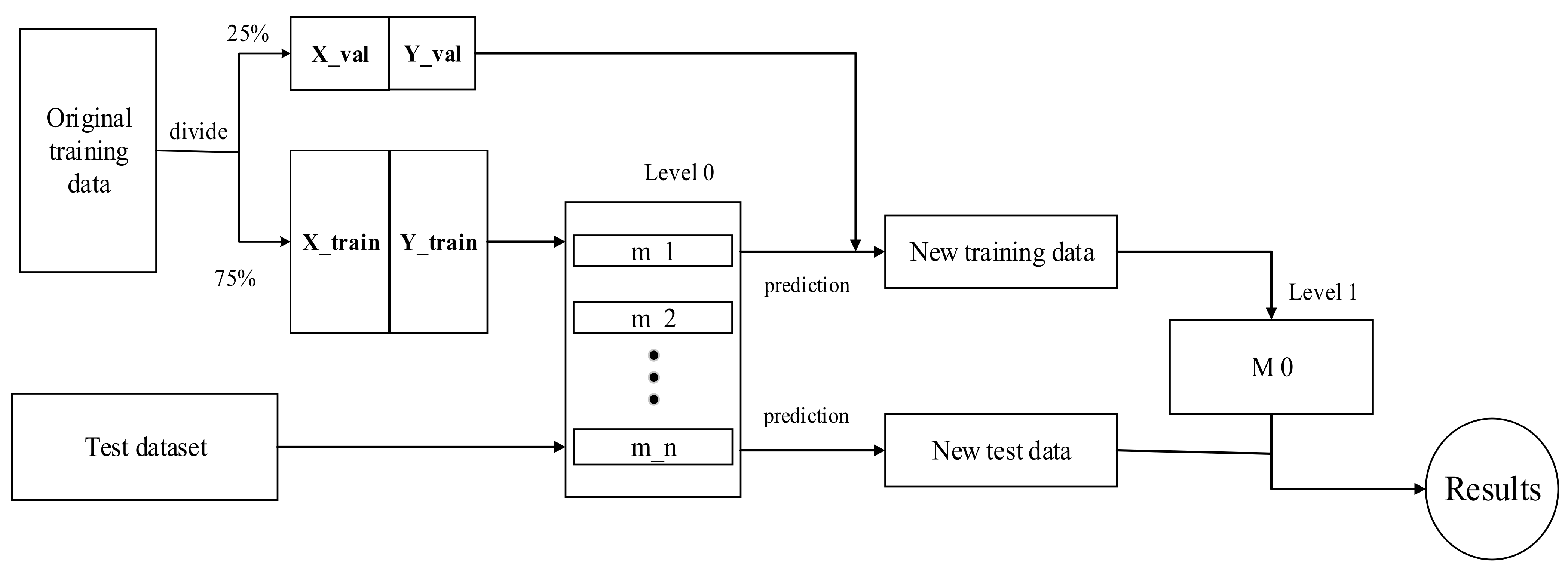
Blending is a technique for combining multiple sub-learners to form a model ensemble. The first layer of the Blending model involves partitioning the training set into a training set and a test set. Multiple models, homogeneous or heterogeneous, can be selected in the first layer. These models are trained using the training sets, and their performance is evaluated on a validation set to obtain the prediction features. These prediction features are then used as the training set for the second layer, where the meta-learner (M0) is directly based on the prediction results of the first level (Figure A1). In this study, the training set is further divided into a first-level training set and a first-level validation set, and sub-learner models such as CatBoost, XGBoost, LightGBM, GB, and KNN are trained on the first-level training set. The trained models are used to predict the validation and test sets. The prediction results of the validation set are used as new features to train the M0 model, while the prediction results of the first test set are used as the test set for the second input to obtain the final prediction results. The remaining 25% of the data is used for testing, while the original data is split 3:1 for training and testing.
Typically, targeting multiple disadvantaged learners g 1 , g 2 , g 3 g t , uniform fusion is suitable when individual learners have similar performance.
G x = 1 T t = 1 T g t x
When the performance of individual learners varies considerably, a weighted average is used to give each g i a different weight to achieve better results.
G x = s i g n t = 1 T α t g t x w i t h α t 0
Use the mean square error to determine α t .
min α t 0 1 n n = 1 N y n t = 1 T α t g t x n 2
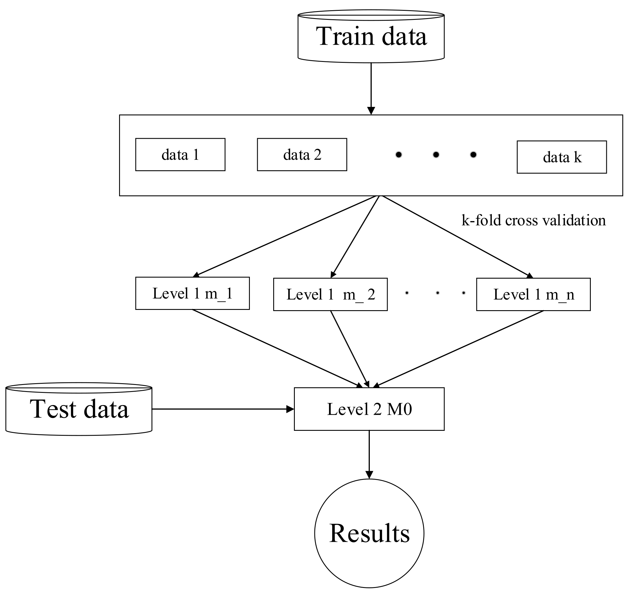
The implementation process of the stacking model (Figure A2) is similar to simple averaging and weighted averaging, in which multiple models are aggregated using a multi-layer structure. This multi-layer stacking architecture is trained layer by layer greedily, first training shallow learner parameters and then gradually training deep learner parameters [40]. The characteristic of the stacking architecture is that it does not directly train all training datasets, but instead it uses k-fold cross validation method to divide the entire training dataset into k equal subsets. In one training session, one of the subsets is used as the test set, while the remaining K-1 subsets are used to train the model. After K cross validation sessions, the output of the Level 1 model on the entire training dataset is obtained [41].

2.4. Model Accuracy Measure

The metrics used to evaluate the model fit and generalization ability are the coefficient of determination (R2), root mean squared error (RMSE), and mean absolute percentage error (MAPE).
R 2 = 1 i = 1 n y ^ i y i i = 1 n y i y ¯ 2
The determination coefficient is used to express the degree of correlation between the predicted value of the model and the measured value. The value is between 0 and 1. The closer the value is to 1, the higher the degree of correlation. On the contrary, the closer the value is to 0, the lower the degree of correlation.
RMSE = i = 1 n y i y ^ i 2 n
The root mean square error is a measure of the deviation of the model from the observed value to the true value. The smaller the RMSE value, the better the result.
MAPE = 1 n y ^ i y i y i
MAPE avoids the situation in which positive and negative errors cancel each other out, and it can reflect the difference between the predicted and measured values more realistically. Usually, MAPE ≤ 0.2 indicates good model robustness; 0.2 < MAPE ≤ 0.5 indicates average model robustness.

2.5. Feature Importance Measure

Assessing the degree of influence of features on prediction results can be achieved using feature importance. A higher importance value for a feature indicates a greater significance in the prediction result. The SHAP method is an effective way of explaining models by measuring the impact of features on model output results through the calculation of importance value for each feature in the sample. It is a versatile method that can be applied to various models [42].
The calculation process of this method is as follows: firstly, the feature subset S is obtained by arranging and combining from the feature set to determine the decision path of the samples. Then, calculate the internal node coverage value according to the sample number of leaf nodes, and then combine the decision path and the internal node coverage value to derive the edge weight. If the feature in the current node is in S, directly follow the path to the next node, and the edge weight is set to 1. If the current node feature is not in S, it needs to traverse its left and right nodes at the same time, and the weight is set to the number of samples of corresponding child nodes or the number of parent nodes. Finally, we return from the leaf node to the root node, and the final value taken at the root node is used as the estimate of f x S [43]. The SHAP value Φ i of feature i is expressed by the formula:
Φ i = S N \ i S ! M S 1 ! M ! f x S i f x S
where N is the set of all features in the training set with dimension M, and S is the subset drawn from N with dimension S .

2.6. Kriging

After predicting the heavy metal content of the sample points, the Kriging interpolation method was used to draw a spatial distribution map of Pb and Cd in the studied soil, with the weight being the average of the observed values based on the degree of spatial correlation. The Kriging method is a spatially localized interpolation method based on the theory of variational functions and structural analysis [44]. Unbiased optimal estimation of regional variables in a limited area is applicable to the spatial correlation of regionalized variables. The realization principle is to use the original data of regionalized variables and the structural characteristics of variogram to conduct linear unbiased optimal estimation of unknown samples [45]. That is, the attribute value of a point is related to the attribute value of its surrounding points, and it can be inferred from the attribute value of its surrounding points. The estimated value z 0 of an unknown issue x 0 , y 0 is a weighted sum of some known points.
z 0 = i = 1 n z i w i
where n is the number of points that can determine the attribute value of the point, z i is the attribute value of the i known point, and w i is the weight of the i known point.

3. Results

3.1. Statistical Characteristics of Heavy Metal Content of Sample Soil

Descriptive statistical data for heavy metals in soil are as follows (Table 1), which includes the mean value, standard deviation, minimum value, maximum value, and coefficient of variation. The correlation coefficient between Pb and Cd is high, with a value of 0.866, indicating that they have a high degree of homology. The coefficient of variation (CV) of Pb is higher compared to Cd, suggesting that Pb concentrations are more variable across the sampled locations. The soil background values in Henan Province from the “Background Values of Elements in Chinese Soils” are taken as the reference values.

3.2. Spectral Feature Extraction

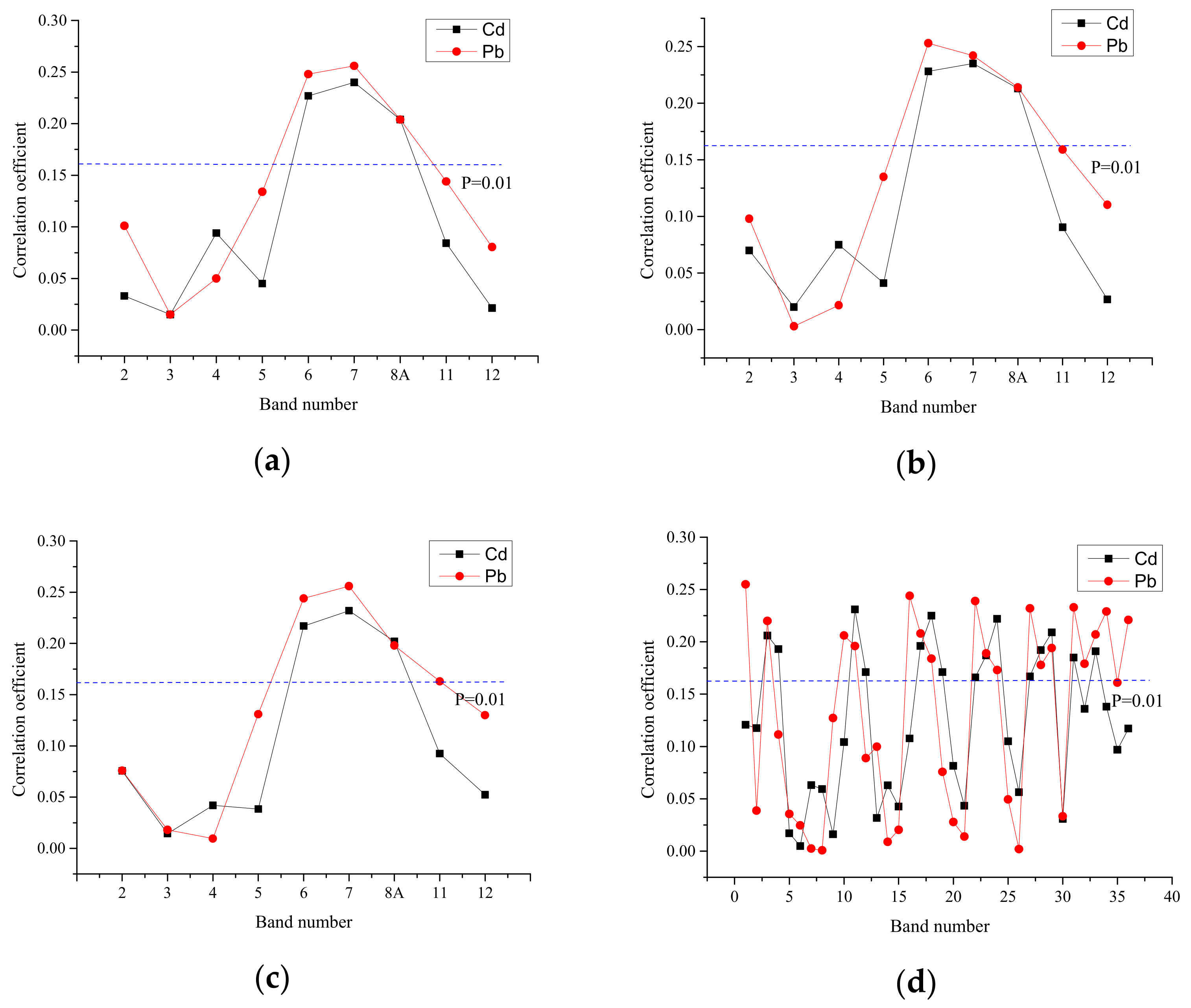
The correlation between the converted spectral bands and the measured values of Pb and Cd contents in soil heavy metals was analyzed using Pearson correlation. The absolute values of these results were used to evaluate the correlation between spectral bands and soil heavy metals (Figure 2).
When the significance level p is greater than 0.01, spectral bands highly correlated with heavy metal content are selected as the spectral characteristics of the model. In the original spectral segment of Sentinel-2A remote sensing image, the B6 to B8A bands are highly correlated with heavy metal content, with the highest correlation coefficient between the original spectral segment B7 and heavy metal content. After logarithmic transformation of spectral reflectance, the correlation coefficient has a slight improvement, and the spectral bands ln6~lnB8A have the highest correlation coefficient with heavy metal content. The overall correlation between the spectral factors and the contents of heavy metals Pb and Cd is negative after the reciprocal operation. However, neither of these conversion methods achieves additional spectral information for the reflection peak and absorption valley. The correlation coefficient band after the band ratio conversion fluctuates greatly between positive and negative values. After ratio calculation, there are 18 spectral factors with a significant level of Pb element greater than 0.01, and there are 13 spectral factors with a significant level of Cd element greater than 0.01.

3.3. Model Estimation and Comparisons

In this study, spectral parameters were selected as characteristic variables using correlation analysis. Spatial and topographical features were also introduced to develop a soil heavy metal content retrieval model based on ensemble learning. A total of 235 sampling points were measured, of which 176 were randomly selected for training, and the remaining 59 were used for prediction, with a ratio of 3:1. In addition to evaluating the proposed model, the results are also compared with traditional regression models such as SVM and RF. The heterogeneous integration learning model establishes an inversion model after adjusting the parameters of the training learner. First, adjust the parameters of the Level 0 learner, determine the parameters, and then adjust the Level 1 learner parameters. Finally, input the prediction dataset into the model to evaluate the model accuracy. Additionally, separately count the best performance of each sub learner.
The model evaluation results are summarized (Table 2). In the inversion model established using spectral characteristics, the R2 value of the Cd element SVM model is relatively low, which means that the model cannot quantitatively estimate the Cd concentration in soil. In addition, the MAPE values of lead and cadmium in all models are greater than 0.5, indicating that the inversion model constructed using Sentinel multispectral bands has low robustness and poor prediction accuracy. With the introduction of spatial and topographic features, various accuracy evaluation indicators have greatly improved. The R2, RMSE, and MAPE of the mixed model that performed best for Pb were 0.9486, 28.5708, and 0.1723, respectively. The R2, RMSE, and MAPE of the mixed model that performed best on Cd elements were 0.9489, 0.3169, and 0.1911, respectively. The MAPE values of the target elements are all less than 0.2, so the hybrid prediction model based on spectral, spatial, and topographic features has high accuracy and stability, and it can be well applied to the study area.

3.4. Feature Importance Analysis

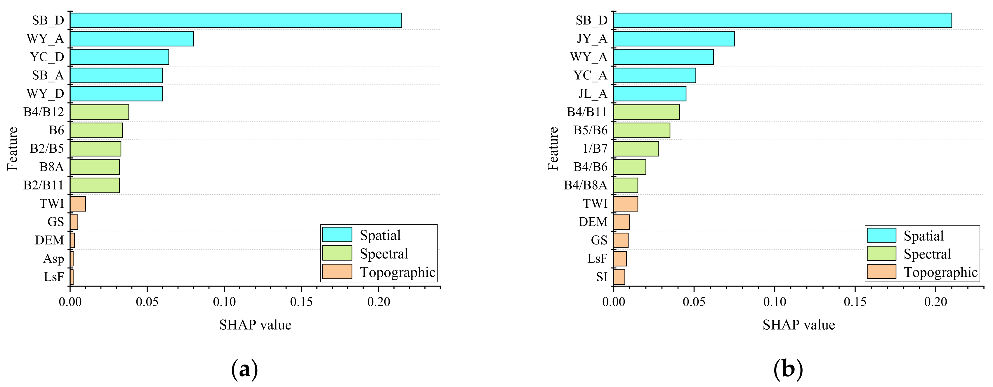
SHAP values are used to evaluate the contribution of spectral, topographic, and spatial characteristics to the construction of heavy metal content inversion models. The article provides the SHAP values of 15 features (Figure 3), which are the features with the highest importance among the three modeling features. The spatial distance feature (SB_D) between the pollution source Shibin smelter and the sampling point is the feature with the greatest contribution in heavy metal Pb and Cd modeling. In addition, the overall SHAP value of spatial features is significantly higher than spectral and topographic features, and topographic features also have a certain positive impact on the model, but their overall impact is weaker compared to spatial and spectral features.

3.5. Spatial Distribution of Heavy Metal Contamination

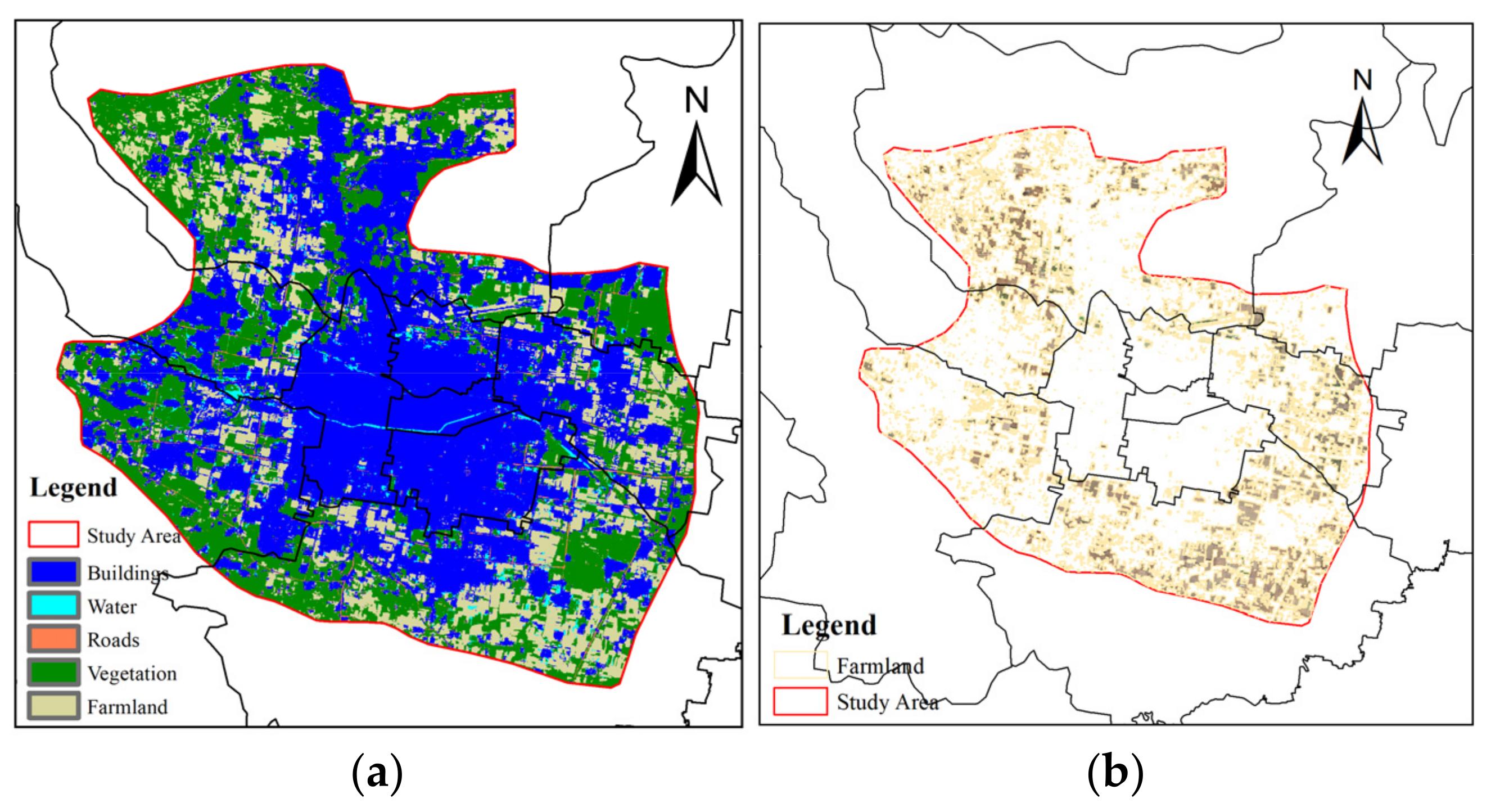
In addition to evaluating the accuracy of the model, it is essential to analyze the spatial trend of heavy metal concentration for a more comprehensive understanding of the distribution of heavy metals Pb and Cd. To achieve this, spatial interpolation of soil heavy metal distribution was performed in the study area. This method provided a visual representation of the heavy metal concentration and its spatial distribution in the study area. To obtain accurate data, the features of the image of the study area were classified using support vector machine (SVM) and artificial vision interpretation [46]. This classification process involved dividing the image into several categories such as vegetation, water, buildings, roads, and farmland (Figure 4). Through this process, the range of farmland in the image was determined, allowing us to conduct a more precise analysis of the distribution of heavy metals in farmland areas.
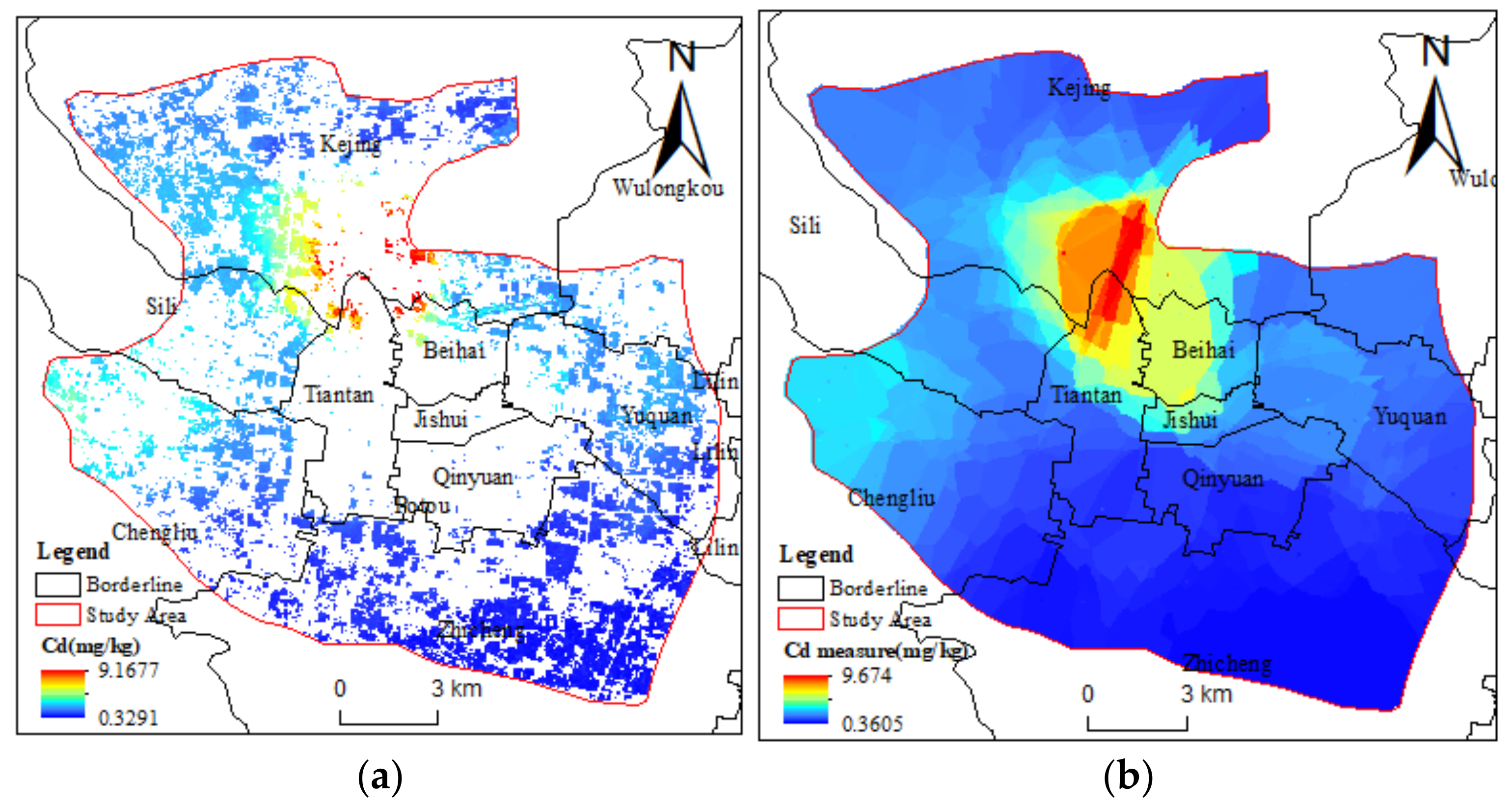
The present study utilized a comprehensive approach to analyze the spatial distribution of heavy metal content in the farmland of the study area. The extraction of spectral, spatial, and topographic features of farmland pixels, along with the robust blending ensemble learning model, proved to be effective in predicting heavy metal content in the farmland. To further evaluate the model performance, Kriging interpolation of measured heavy metal content was performed to obtain the spatial distribution of heavy metal content in the entire study area [47]. The spatial distribution of the predicted content of Pb and Cd based on Sentinel-2A (Figure 5a and Figure 6a) was in good agreement with the actual measured value (Figure 5b and Figure 6b), as verified by the comparison of the spatial distribution of measured and predicted heavy metal content. These findings suggest the feasibility of using Sentinel-2A remote sensing images to accurately predict heavy metal content in soils. Overall, the study provides an innovative and reliable approach for analyzing the spatial distribution of heavy metals in farmland using remote sensing images and machine learning models.
The correlation analysis results show that Pb and Cd have a high degree of homology, so the interpretation of Pb prediction results overlaps with the understanding of Cd prediction results. Based on the comparison between the measured heavy metal content and the spatial distribution of heavy metal content predicted by Sentinel-2A, it can be found that the soil heavy metal content in the northwest of the study area is relatively high, and the soil heavy metal content shows a downward trend from northwest to southeast.

4. Discussion

4.1. Soil Heavy Metal Contents

In this study, we aimed to map the spatial distribution of heavy metal concentrations in Jiyuan and its surrounding areas using Sentinel-2A data. Our results showed that the coefficients of variation for heavy metals Pb and Cd were 109 and 96%, respectively, indicating that the distribution of heavy metal concentration is heavily influenced by human activities. These findings are consistent with those of previous studies. For example, Wang et al. [48] investigated the spatial distribution and accumulation of heavy metals in Chinese soil, and they found that the content of cadmium in soil is generally lower than the average concentration of 2.155 mg/kg observed in our study. Similarly, the research results of Pan et al. [49] on heavy metals in cities showed that the median concentration of Pb was slightly lower than the minimum concentration range of Pb measured in our study. Our statistical analysis revealed a high correlation coefficient of 0.866 between Cd and Pb content, indicating their strong homology and potential for synergistic effects, which is consistent with existing research on heavy metal correlations [50]. By comparing the spatial distribution of Pb content derived from Sentinel-2A data with that of Cd content derived from Sentinel-2A data, we found that the distribution of Cd content is similar to that of Pb content.

4.2. Comparison Prediction Performance of Models

Comparing the performance of traditional regression models and integrated models in predicting heavy metal concentrations in soil, it was found that the integrated model outperforms RF and SVM in predicting heavy metal content. This is because there is a non-linear relationship between modeling factors and heavy metals, while SVM is a linear regression algorithm that has a slightly weaker ability to quantitatively estimate the content of heavy metals in soil [51]. On the other hand, the RF and gradient boosting (GB) models are both regression models based on decision trees and perform well in predicting heavy metal content [52]. Studies have shown that models based on heterogeneous integration can overcome various problems caused by small sample sets and unbalanced data [53]. The Stacking model may use global statistical features when training on part of the data, leading to a distorted model performance. The Blending model only needs to train different base models on non-overlapping data, and the output values are weighted averages, avoiding information leakage. Model prediction results show that the Blending model based on heterogeneous ensembles performs best among all models, with R2 values of 0.9486 and 0.9489 for the two heavy metals Pb and Cd, respectively.
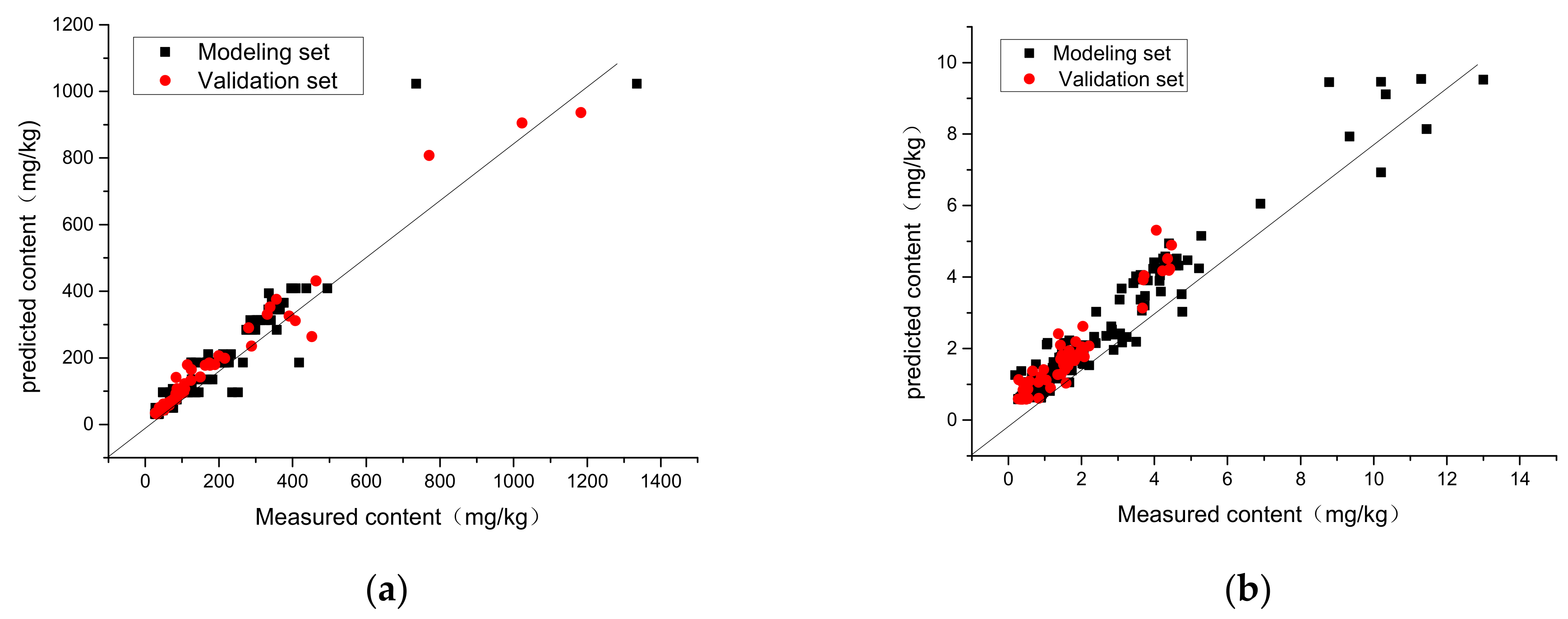
A regression analysis was conducted to evaluate the performance of the optimal model in predicting heavy metal Pb and Cd concentrations. A 1:1 relationship plot was generated by plotting the predicted values against the measured values. As demonstrated in Section 3.3, the hybrid models that integrate spectral, spatial, and topographic features achieved the best accuracy evaluation indicators for heavy metal inversion. The x-axis of the plot indicates the measured values of heavy metals at the sample point, while the y-axis represents the predicted values of the hybrid model (Figure 7).
In the heavy metal inversion scatter diagram, the predicted and measured values of the Blending model in the training and test sets are both almost a 1:1 straight line, indicating that the fitting effect is good [54], and the predicted values of soil Pb and Cd content obtained from inversion are relatively reasonable, which can be used to monitor the soil Pb and Cd content values in the study area and provide a basis for soil environmental monitoring.

4.3. Impact of Topography and Spatial Factors

After extracting spectral reflectance from sample points in Sentinel-2A multispectral remote sensing images, a soil heavy metal Pb and Cd content prediction model was developed by incorporating spatial and topographic characteristics of pollution sources and sinks. The model’s performance was significantly improved compared to using Sentinel spectral single features, which supports our hypothesis. Inorganic pollutants generated during mining and metal smelting are predominantly point source pollution that spreads due to natural factors such as wind direction, wind speed, terrain, and precipitation [55]. Previous studies have investigated the contribution of source landscapes using atmospheric sedimentation and surface runoff as diffusion paths to the accumulation of heavy metals in soil [56]. The spatial distribution of heavy metals typically follows the terrain [57], but the study area’s overall terrain is relatively flat, with no significant elevation fluctuations, and thus, topographic characteristics have a weak impact on the spatial heterogeneity of heavy metals. The spatial distribution of heavy metals in soil is influenced by a combination of environmental factors [58]. Soil samples were collected from cultivated land around towns in the study area, and the five metal smelters distributed in the area are the primary reasons for the high-value areas of heavy metals in the soil. Correlation analysis between heavy metal content and spatial and topographic features (Table A1 and Table A2) reveals that ten spatial features are negatively correlated with heavy metal content. As the distance from the pollution source increases, areas with high heavy metal content gradually disappear.

4.4. Heavy Metal Concentration Distribution

The accumulation of heavy metals in soil can result from various sources, including fertilization, agricultural chemicals, atmospheric sedimentation, sewage irrigation, mining, metal ore, sludge application, smelting operations of industrial waste, fossil fuel refining and combustion, and remodification [59]. China’s rapid industrialization and urbanization over the past three decades have been identified as the primary factor contributing to the increased presence of heavy metals in soil [60]. In particular, industrial emissions from heavy metal smelting are a significant source of heavy metal pollution in soil, as several metal smelters are distributed throughout the study area [61]. The spatial distribution of heavy metals in soil is characterized by diffusion around the center of metal smelters, likely resulting from atmospheric diffusion deposition and rainfall [62]. The target areas with high heavy metal content are located in the south of Kejing Town and the north of Chengliu Town, both of which are near metal smelters. During the smelting process of heavy metals, lead in wastewater, waste residue, and atmospheric dust gradually migrates to cultivated land and accumulates continuously, resulting in lead pollution of cultivated land soil [63]. According to a study by Zhang et al. [64], the pollution rate of heavy metals in farmland soils is the highest for Cd, followed by Hg, Cu, Ni, Zn, and Pb, while Cr has the lowest pollution rate. The total pollution rate of farmland soil is primarily attributed to Cd, Hg, Cu, and Ni. In the study area, sludge is being used for irrigation, gradually accumulating heavy metals such as Pb and Cd in the farmland. The use of pesticides, fertilizers, and plastic mulch can also cause the accumulation of heavy metals in soil [65,66]. Agricultural plastic films, for instance, contain heat stabilizers with heavy metals such as Cd and Pb, which can result in heavy metal pollution during their use in plastic greenhouses and mulching [67]. The widespread use of electronic equipment generates a substantial amount of electronic waste that contains heavy metals (Cd, Co, Ni, and Pb) [68]. In the main urban area of Jiyuan, human activities, domestic garbage, and industrial waste are the primary sources of heavy metal pollution. Pb and Cd in vehicle exhaust are deposited into road soil through the atmosphere, resulting in a zonal distribution of Pb content in soil on both sides of the road [69]. In the study area, low-value areas of heavy metal content are mainly distributed in the south of Chengliu Town, Yuquan Street, and Heji Town in the northeast of Kejing Town, which are far away from metal smelters and main urban areas and thus have high soil environmental quality.

5. Conclusions

This article takes the surrounding area of Jiyuan City, Henan Province, China as the research area, collects 235 soil sample data on the spot, conducts chemical analysis, obtains the heavy metal content of the samples, and constructs an inversion model using Sentinel-2A multi spectral images, spatial features of pollution source-sinks and topographic factors. Compared with many traditional models, the prediction accuracy of blending ensemble learning model is evaluated.
The experiments show that the model constructed by the blending method has obvious advantages, among which the test set R2 of Pb’s Blending model is 0.9486, the Blending model R2 of Cd is 0.9489, and the MAPE value is less than 0.2. The high estimation accuracy of the Blending soil heavy metal estimation model shows that this method is highly feasible for the inversion of soil heavy metal content. The paper proposes to construct the spatial features of potential pollution sources to quantify the spatial influence factors of pollutant diffusion, and the method is applicable to point source and line source pollution with clear sources of pollutants. Generally, soil heavy metal pollutants such as atmospheric dust and sewage discharge originate from mining activities, metallurgy, and industrial production, and the sources of pollution are clear. Therefore, the proposed method has high popularization and application potential.

Author Contributions

Conceptualization, H.Y. and S.X.; writing—original draft preparation, H.Y. and S.X.; writing—review and editing, P.L., P.J., C.S. and Z.H. All authors have read and agreed to the published version of the manuscript.

Funding

This research was funded by National Natural Science Foundation Program (U1304402, 41977284) and Natural Science and Technology Program of Henan Provincial Department of Natural Resources (2019-378-16).

Data Availability Statement

Not applicable.

Conflicts of Interest

The authors declare no conflict of interest.

Appendix A

Table A1. Correlation coefficient between Pb content and spatial and topographic characteristics.
Spatial FeatureCorrelation CoefficientTopography FeatureCorrelation Coefficient
JL_D−0.26 9 **DEM0.062
JL_A−0.502 **MF−0.063
JY_D−0.168 **GS0.061
JY_A−0.397 **Sl−0.139 *
SB_D−0.653 **Asp0.013
SB_A−0.370 **WE−0.091
WY_A−0.501 **LsF−0.044
WY_B−0.506 **TWI−0.096
YC_D−0.552 **
YC_A−0.259 **
**: extremely significant correlation markersstandard deviation; *: significant correlation markers.
Table A2. Correlation coefficient between Cd content and spatial and topographic characteristics.
Spatial FeatureCorrelation CoefficientTopography FeatureCorrelation Coefficient
JL_D−0.289 **DEM0.110
JL_A−0.482 **MF−0.072
JY_D−0.243 **GS0.109
JY_A−0.426 **Sl−0.094
SB_D−0.628 **Asp0.027
SB_A−0.209 **WE−0.053
WY_A−0.461 **LsF−0.041
WY_B−0.497 **TWI−0.140 *
YC_D−0.519 **
YC_A−0.141 **
**: extremely significant correlation markersstandard deviation; *: significant correlation markers.
Figure A1. Blending model.
Remotesensing 15 02299 g0a1
Figure A2. Stacking model.
Remotesensing 15 02299 g0a2

References

  1. Järup, L. Hazards of heavy metal contamination. Br. Med. Bull. 2003, 68, 167–182. [Google Scholar] [CrossRef]
  2. The Report on the National General Survey of Soil Contamination. Available online: http://www.gov.cn/foot/site1/20140417/782bcb88840814ba158d01.pdf (accessed on 14 January 2019).
  3. Zhong, X.; Chen, Z.; Li, Y.; Ding, K.; Liu, W.; Liu, Y.; Yuan, Y.; Zhang, M.; Baker, A.J.; Yang, W. Factors influencing heavy metal availability and risk assessment of soils at typical metal mines in Eastern China. J. Hazard. Mater. 2020, 400, 123289. [Google Scholar] [CrossRef] [PubMed]
  4. Chen, T.; Chang, Q.; Liu, J.; Clevers, J.; Kooistra, L. Identification of soil heavy metal sources and improvement in spatial mapping based on soil spectral information: A case study in northwest China. Sci. Total Environ. 2016, 565, 155–164. [Google Scholar] [CrossRef] [PubMed]
  5. Kooistra, L.; Wanders, J.; Epema, G.; Leuven, R.; Wehrens, R.; Buydens, L. The potential of field spectroscopy for the assessment of sediment properties in river floodplains. Anal. Chim. Acta 2003, 484, 189–200. [Google Scholar] [CrossRef]
  6. Fang, Y.; Xu, L.; Wong, A.; Clausi, D.A. Multi-Temporal Landsat-8 Images for Retrieval and Broad Scale Mapping of Soil Copper Concentration Using Empirical Models. Remote Sens. 2022, 14, 2311. [Google Scholar] [CrossRef]
  7. Govender, M.; Chetty, K.; Naiken, V.; Bulcock, H. A comparison of satellite hyperspectral and multispectral remote sensing imagery for improved classification and mapping of vegetation. Water SA 2008, 34, 147–154. [Google Scholar] [CrossRef]
  8. Khosravi, V.; Gholizadeh, A.; Saberioon, M. Soil toxic elements determination using integration of Sentinel-2 and Landsat-8 images: Effect of fusion techniques on model performance. Environ. Pollut. 2022, 310, 119828. [Google Scholar] [CrossRef]
  9. Soodan, R.K.; Pakade, Y.B.; Nagpal, A.; Katnoria, J.K. Analytical techniques for estimation of heavy metals in soil ecosystem: A tabulated review. Talanta 2014, 125, 405–410. [Google Scholar] [CrossRef]
  10. Yang, Y.; Cui, Q.; Jia, P.; Liu, J.; Bai, H. Estimating the heavy metal concentrations in topsoil in the Daxigou mining area, China, using multispectral satellite imagery. Sci. Rep. 2021, 11, 11718. [Google Scholar] [CrossRef]
  11. Gang, S.; Wenjiang, H.; Pengfei, C.; Shuai, G.; Xiu, W. Advances in UAV-based multispectral remote sensing applications. Nongye Jixie Xuebao/Trans. Chin. Soc. Agric. Mach. 2018, 49, 3. [Google Scholar]
  12. Kobayashi, N.; Tani, H.; Wang, X.; Sonobe, R. Crop classification using spectral indices derived from Sentinel-2A imagery. J. Inf. Telecommun. 2020, 4, 67–90. [Google Scholar] [CrossRef]
  13. Li, J.; Roy, D.P. A global analysis of Sentinel-2A, Sentinel-2B and Landsat-8 data revisit intervals and implications for terrestrial monitoring. Remote Sens. 2017, 9, 902. [Google Scholar] [CrossRef]
  14. Guo, M.; Yu, Z.; Xu, Y.; Huang, Y.; Li, C. ME-net: A deep convolutional neural network for extracting mangrove using sentinel-2A data. Remote Sens. 2021, 13, 1292. [Google Scholar] [CrossRef]
  15. Navarro, G.; Caballero, I.; Silva, G.; Parra, P.-C.; Vázquez, Á.; Caldeira, R. Evaluation of forest fire on Madeira Island using Sentinel-2A MSI imagery. Int. J. Appl. Earth Obs. Geoinf. 2017, 58, 97–106. [Google Scholar] [CrossRef]
  16. Zhao, H.; Liu, P.; Qiao, B.; Wu, K. The spatial distribution and prediction of soil heavy metals based on measured samples and multi-spectral images in Tai Lake of China. Land 2021, 10, 1227. [Google Scholar] [CrossRef]
  17. Zhiyuan, W.; Dengfeng, W.; Huiping, Z.; Zhiping, Q. Assessment of soil heavy metal pollution with principal component analysis and geoaccumulation index. Procedia Environ. Sci. 2011, 10, 1946–1952. [Google Scholar] [CrossRef]
  18. Zhou, W.; Yang, H.; Xie, L.; Li, H.; Huang, L.; Zhao, Y.; Yue, T. Hyperspectral inversion of soil heavy metals in Three-River Source Region based on random forest model. Catena 2021, 202, 105222. [Google Scholar] [CrossRef]
  19. Xian-Li, X.; Xian-Zhang, P.; Bo, S. Visible and near-infrared diffuse reflectance spectroscopy for prediction of soil properties near a copper smelter. Pedosphere 2012, 22, 351–366. [Google Scholar]
  20. Choe, E.; van der Meer, F.; van Ruitenbeek, F.; van der Werff, H.; de Smeth, B.; Kim, K.-W. Mapping of heavy metal pollution in stream sediments using combined geochemistry, field spectroscopy, and hyperspectral remote sensing: A case study of the Rodalquilar mining area, SE Spain. Remote Sens. Environ. 2008, 112, 3222–3233. [Google Scholar] [CrossRef]
  21. Kemper, T.; Sommer, S. Estimate of heavy metal contamination in soils after a mining accident using reflectance spectroscopy. Environ. Sci. Technol. 2002, 36, 2742–2747. [Google Scholar] [CrossRef]
  22. Goodarzi, R.; Mokhtarzade, M.; Valadan Zoej, M.J. A robust fuzzy neural network model for soil lead estimation from spectral features. Remote Sens. 2015, 7, 8416–8435. [Google Scholar] [CrossRef]
  23. Liu, H.; Xiong, Z.; Jiang, X.; Liu, G.; Liu, W. Heavy metal concentrations in riparian soils along the Han River, China: The importance of soil properties, topography and upland land use. Ecol. Eng. 2016, 97, 545–552. [Google Scholar] [CrossRef]
  24. Alloway, B.J. Sources of Heavy Metals and Metalloids in Soils. In Heavy Metals in Soils; Springer: Berlin/Heidelberg, Germany, 2013; pp. 11–50. [Google Scholar]
  25. Gascon, F.; Bouzinac, C.; Thépaut, O.; Jung, M.; Francesconi, B.; Louis, J.; Lonjou, V.; Lafrance, B.; Massera, S.; Gaudel-Vacaresse, A. Copernicus Sentinel-2A calibration and products validation status. Remote Sens. 2017, 9, 584. [Google Scholar] [CrossRef]
  26. Li, L.; Zhou, X.; Chen, L.; Chen, L.; Zhang, Y.; Liu, Y. Estimating urban vegetation biomass from Sentinel-2A image data. Forests 2020, 11, 125. [Google Scholar] [CrossRef]
  27. Djamai, N.; Fernandes, R. Comparison of SNAP-derived Sentinel-2A L2A product to ESA product over Europe. Remote Sens. 2018, 10, 926. [Google Scholar] [CrossRef]
  28. Gitahi, J.; Hahn, M.; Ramirez, A. High-resolution urban aerosol monitoring using Sentinel-2 satellite images. Earth Obs. Geomat. Eng. 2019, 3, 102–111. [Google Scholar]
  29. Li, Y.; Chen, J.; Ma, Q.; Zhang, H.K.; Liu, J. Evaluation of Sentinel-2A surface reflectance derived using Sen2Cor in North America. IEEE J. Sel. Top. Appl. Earth Obs. Remote Sens. 2018, 11, 1997–2021. [Google Scholar] [CrossRef]
  30. Warren, M.A.; Simis, S.G.; Martinez-Vicente, V.; Poser, K.; Bresciani, M.; Alikas, K.; Spyrakos, E.; Giardino, C.; Ansper, A. Assessment of atmospheric correction algorithms for the Sentinel-2A MultiSpectral Imager over coastal and inland waters. Remote Sens. Environ. 2019, 225, 267–289. [Google Scholar] [CrossRef]
  31. Zhang, M.; Zhang, M.; Yang, H.; Jin, Y.; Zhang, X.; Liu, H. Mapping regional soil organic matter based on sentinel-2a and modis imagery using machine learning algorithms and google earth engine. Remote Sens. 2021, 13, 2934. [Google Scholar] [CrossRef]
  32. Dokmanic, I.; Parhizkar, R.; Ranieri, J.; Vetterli, M. Euclidean distance matrices: Essential theory, algorithms, and applications. IEEE Signal Process. Mag. 2015, 32, 12–30. [Google Scholar] [CrossRef]
  33. Brümmer, G. Heavy Metal Species, Mobility and Availability in Soils. In The Importance of Chemical “Speciation” in Environmental Processes; Springer: Berlin/Heidelberg, Germany, 1986; pp. 169–192. [Google Scholar]
  34. Bolstad, P.V.; Stowe, T. An evaluation of DEM accuracy: Elevation, slope, and aspect. Photogramm. Eng. Remote Sens. 1994, 60, 1327–1332. [Google Scholar]
  35. Panagos, P.; Borrelli, P.; Meusburger, K. A new European slope length and steepness factor (LS-Factor) for modeling soil erosion by water. Geosciences 2015, 5, 117–126. [Google Scholar] [CrossRef]
  36. Wang, X.-C.; Klemeš, J.J.; Dong, X.; Fan, W.; Xu, Z.; Wang, Y.; Varbanov, P.S. Air pollution terrain nexus: A review considering energy generation and consumption. Renew. Sustain. Energy Rev. 2019, 105, 71–85. [Google Scholar] [CrossRef]
  37. Plaza, E.; Aamodt, A.; Ram, A.; Velde, W.; Someren, M.v. Integrated learning architectures. In Proceedings of the European Conference on Machine Learning, Vienna, Austria, 5–7 April 1993; pp. 427–441. [Google Scholar]
  38. Sutton, C.D. Classification and regression trees, bagging, and boosting. Handb. Stat. 2005, 24, 303–329. [Google Scholar]
  39. Huang, J.-C.; Ko, K.-M.; Shu, M.-H.; Hsu, B.-M. Application and comparison of several machine learning algorithms and their integration models in regression problems. Neural Comput. Appl. 2020, 32, 5461–5469. [Google Scholar] [CrossRef]
  40. Breiman, L. Stacked regressions. Mach. Learn. 1996, 24, 49–64. [Google Scholar] [CrossRef]
  41. Seewald, A.K. How to make stacking better and faster while also taking care of an unknown weakness. In Proceedings of the Proceedings of the Nineteenth International Conference on Machine Learning, San Francisco, CA, USA, 8–12 July 2002; pp. 554–561.
  42. Van den Broeck, G.; Lykov, A.; Schleich, M.; Suciu, D. On the tractability of SHAP explanations. J. Artif. Intell. Res. 2022, 74, 851–886. [Google Scholar] [CrossRef]
  43. Hu, M.; Zhang, H.; Wu, B.; Li, G.; Zhou, L. Interpretable predictive model for shield attitude control performance based on XGboost and SHAP. Sci. Rep. 2022, 12, 1–14. [Google Scholar] [CrossRef]
  44. da Silveira, H.L.F.; Galvão, L.S.; Sanches, I.D.A.; de Sá, I.B.; Taura, T.A. Use of MSI/Sentinel-2 and airborne LiDAR data for mapping vegetation and studying the relationships with soil attributes in the Brazilian semi-arid region. Int. J. Appl. Earth Obs. Geoinf. 2018, 73, 179–190. [Google Scholar] [CrossRef]
  45. Baltas, H.; Yesilkanat, C.M.; Kiris, E.; Sirin, M. A study of the radiological baseline conditions around the planned Sinop (Turkey) nuclear power plant using the mapping method. Environ. Monit. Assess. 2019, 191, 1–14. [Google Scholar] [CrossRef]
  46. Li, X.; Liu, L.; Huang, L. Comparison of several remote sensing image classification methods based on envi. Int. Arch. Photogramm. Remote Sens. Spat. Inf. Sci. 2020, 42, 605–611. [Google Scholar] [CrossRef]
  47. Liao, Y.; Li, D.; Zhang, N. Comparison of interpolation models for estimating heavy metals in soils under various spatial characteristics and sampling methods. Trans. GIS 2018, 22, 409–434. [Google Scholar] [CrossRef]
  48. Dong, W.Q.Y.; Cui, Y.; Liu, X. Instances of soil and crop heavy metal contamination in China. Soil Sediment Contam. 2001, 10, 497–510. [Google Scholar] [CrossRef]
  49. Pan, L.; Wang, Y.; Ma, J.; Hu, Y.; Su, B.; Fang, G.; Wang, L.; Xiang, B. A review of heavy metal pollution levels and health risk assessment of urban soils in Chinese cities. Environ. Sci. Pollut. Res. 2018, 25, 1055–1069. [Google Scholar] [CrossRef] [PubMed]
  50. Cai, L.; Xu, Z.; Ren, M.; Guo, Q.; Hu, X.; Hu, G.; Wan, H.; Peng, P. Source identification of eight hazardous heavy metals in agricultural soils of Huizhou, Guangdong Province, China. Ecotoxicol. Environ. Saf. 2012, 78, 2–8. [Google Scholar] [CrossRef]
  51. Smola, A.J.; Schölkopf, B. A tutorial on support vector regression. Stat. Comput. 2004, 14, 199–222. [Google Scholar] [CrossRef]
  52. Biau, G. Analysis of a random forests model. J. Mach. Learn. Res. 2012, 13, 1063–1095. [Google Scholar]
  53. Tan, K.; Ma, W.; Chen, L.; Wang, H.; Du, Q.; Du, P.; Yan, B.; Liu, R.; Li, H. Estimating the distribution trend of soil heavy metals in mining area from HyMap airborne hyperspectral imagery based on ensemble learning. J. Hazard. Mater. 2021, 401, 123288. [Google Scholar] [CrossRef]
  54. Su, Y.; Guo, B.; Lei, Y.; Zhang, D.; Guo, X.; Suo, L.; Zhao, Y.; Bian, Y. An Indirect Inversion Scheme for Retrieving Toxic Metal Concentrations Using Ground-Based Spectral Data in a Reclamation Coal Mine, China. Water 2022, 14, 2784. [Google Scholar] [CrossRef]
  55. Ding, Q.; Cheng, G.; Wang, Y.; Zhuang, D. Effects of natural factors on the spatial distribution of heavy metals in soils surrounding mining regions. Sci. Total Environ. 2017, 578, 577–585. [Google Scholar] [CrossRef]
  56. Yang, X.; Yang, Y.; Wan, Y.; Wu, R.; Feng, D.; Li, K. Source identification and comprehensive apportionment of the accumulation of soil heavy metals by integrating pollution landscapes, pathways, and receptors. Sci. Total Environ. 2021, 786, 147436. [Google Scholar] [CrossRef]
  57. Zhao, D.; Xie, D.; Yin, F.; Liu, L.; Feng, J.; Ashraf, T. Estimation of Pb Content Using Reflectance Spectroscopy in Farmland Soil near Metal Mines, Central China. Remote Sens. 2022, 14, 2420. [Google Scholar] [CrossRef]
  58. Hou, D.; O’Connor, D.; Nathanail, P.; Tian, L.; Ma, Y. Integrated GIS and multivariate statistical analysis for regional scale assessment of heavy metal soil contamination: A critical review. Environ. Pollut. 2017, 231, 1188–1200. [Google Scholar] [CrossRef]
  59. Zhao, F.-J.; Ma, Y.; Zhu, Y.-G.; Tang, Z.; McGrath, S.P. Soil contamination in China: Current status and mitigation strategies. Environ. Sci. Technol. 2015, 49, 750–759. [Google Scholar] [CrossRef]
  60. Sodango, T.H.; Li, X.; Sha, J.; Bao, Z. Review of the spatial distribution, source and extent of heavy metal pollution of soil in China: Impacts and mitigation approaches. J. Health Pollut. 2018, 8, 53–70. [Google Scholar] [CrossRef]
  61. Pelfrêne, A.; Waterlot, C.; Mazzuca, M.; Nisse, C.; Cuny, D.; Richard, A.; Denys, S.; Heyman, C.; Roussel, H.; Bidar, G. Bioaccessibility of trace elements as affected by soil parameters in smelter-contaminated agricultural soils: A statistical modeling approach. Environ. Pollut. 2012, 160, 130–138. [Google Scholar] [CrossRef]
  62. Li, P.; Wu, T.; Jiang, G.; Pu, L.; Li, Y.; Zhang, J.; Xu, F.; Xie, X. An integrated approach for source apportionment and health risk assessment of heavy metals in subtropical agricultural soils, Eastern China. Land 2021, 10, 1016. [Google Scholar] [CrossRef]
  63. Yan, W.; Liu, D.; Peng, D.; Mahmood, Q.; Chen, T.; Wang, Y.; Li, S.; Chen, J. Spatial distribution and risk assessment of heavy metals in the farmland along mineral product transportation routes in Zhejiang, China. Soil Use Manag. 2016, 32, 338–349. [Google Scholar] [CrossRef]
  64. Cheng, H.; Li, M.; Zhao, C.; Li, K.; Peng, M.; Qin, A.; Cheng, X. Overview of trace metals in the urban soil of 31 metropolises in China. J. Geochem. Explor. 2014, 139, 31–52. [Google Scholar] [CrossRef]
  65. Zeng, X.-B.; Li, L.-F.; Mei, X.-R. Heavy metal content in Chinese vegetable plantation land soils and related source analysis. Agric. Sci. China 2008, 7, 1115–1126. [Google Scholar] [CrossRef]
  66. Atafar, Z.; Mesdaghinia, A.; Nouri, J.; Homaee, M.; Yunesian, M.; Ahmadimoghaddam, M.; Mahvi, A.H. Effect of fertilizer application on soil heavy metal concentration. Environ. Monit. Assess. 2010, 160, 83–89. [Google Scholar] [CrossRef] [PubMed]
  67. Yu, H.; Hou, J.; Dang, Q.; Cui, D.; Xi, B.; Tan, W. Decrease in bioavailability of soil heavy metals caused by the presence of microplastics varies across aggregate levels. J. Hazard. Mater. 2020, 395, 122690. [Google Scholar] [CrossRef] [PubMed]
  68. Zhong, T.; Chen, D.; Zhang, X. Identification of potential sources of mercury (Hg) in farmland soil using a decision tree method in China. Int. J. Environ. Res. Public Health 2016, 13, 1111. [Google Scholar] [CrossRef] [PubMed]
  69. He, L.; Gao, X. Assessment of potential ecological risk for soil heavy metals in Sanjiang Source Region: A case study of Yushu County, Qinghai Province. J. Agro-Environ. Sci 2016, 35, 1071–1080. [Google Scholar]
Figure 1. Study area location and sample distribution (red dots). Green triangles represent towns. Yellow triangles represent metal smelters.
Remotesensing 15 02299 g001
Figure 2. Correlation coefficients of heavy metal content with transformed spectra: (a) raw reflectance; (b) logarithmic operation; (c) inverse operation; (d) band ratio.
Remotesensing 15 02299 g002
Figure 3. Assessment of the importance of spectral, spatial, and topographic features: (a) Results of Pb feature evaluation; (b) Results of Cd feature evaluation.
Remotesensing 15 02299 g003
Figure 4. Study area mask extraction: (a) Classification results of surface features in the study area; (b) Farmland extraction results in the study area.
Remotesensing 15 02299 g004
Figure 5. Spatial distribution of predicted and measured interpolated values of heavy metals: (a) Pb content of Sentinel-2A remote sensing inversions in the study area; (b) Spatial interpolation distribution of measured Pb content.
Remotesensing 15 02299 g005
Figure 6. Spatial distribution of predicted and measured interpolated values of heavy metals: (a) Cd content of Sentinel-2A remote sensing inversions in the study area; (b) Spatial interpolation distribution of measured Cd content.
Remotesensing 15 02299 g006
Figure 7. Scatter plot of the measured and predicted value. (a) Soil Pb content; (b) soil Cd content.
Remotesensing 15 02299 g007
Table 1. Descriptive statistics of soil heavy Pb and Cd Concentration (Unit: mg/kg).
MetalNumberMinMaxMeanSD 1CV 2SBV 3
Pb23526.541335158.6174.21.0919.6
Cd2350.19132.1552.0710.960.074
1 SD: standard deviation; 2 CV: coefficient of variation; 3 SBV: the soil background value.
Table 2. Comparison of model accuracy based on spectral features.
FeatureModelPbCd
RMSER2MAPERMSER2MAPE
SpectrumRF80.68730.59020.73071.05790.43070.8403
SVM152.94960.20170.71632.09680.09780.8107
KNN98.26690.67970.69741.38830.49950.6620
GBR92.56420.71580.64911.24120.60000.5388
XGBoost88.56360.73980.53431.25680.58980.5436
LightGBM93.50860.71000.70191.34560.52980.6201
CatBoost86.35910.75260.58581.21390.61740.5694
Stacking85.11860.75970.50931.44500.45780.6747
Blending83.80550.76700.58581.18450.63560.5471
Spectrum +
Topography
+ Spatial
RF35.53210.92050.18680.42590.90770.2812
SVM119.52490.36090.31600.80750.62840.3695
KNN29.86340.94390.16500.33680.94230.1634
GBR34.05590.92700.23390.47660.88440.3218
XGBoost30.72700.94060.20200.35830.93470.1952
LightGBM35.59110.92030.21270.43610.90330.3199
CatBoost38.46220.90690.26990.43130.90540.2986
Stacking36.19740.91750.17260.43000.90600.2774
Blending28.57080.94860.17230.31690.94890.1911
Disclaimer/Publisher’s Note: The statements, opinions and data contained in all publications are solely those of the individual author(s) and contributor(s) and not of MDPI and/or the editor(s). MDPI and/or the editor(s) disclaim responsibility for any injury to people or property resulting from any ideas, methods, instructions or products referred to in the content.