Article

Thermal Discharge Temperature Retrieval and Monitoring of NPPs Based on SDGSAT-1 Images

1
Hangzhou Institute for Advanced Study, University of Chinese Academy of Sciences, Hangzhou 310024, China
2
University of Chinese Academy of Sciences, Beijing 100049, China
3
State Key Laboratory of Infrared Physics, Shanghai Institute of Technical Physics, Chinese Academy of Sciences, 500 Yu Tian Road, Shanghai 200083, China
4
International Research Center of Big Data for Sustainable Development Goals (CBAS), Beijing 100094, China
*
Author to whom correspondence should be addressed.
Remote Sens. 2023, 15(9), 2298; https://doi.org/10.3390/rs15092298
Submission received: 22 February 2023 / Revised: 15 April 2023 / Accepted: 25 April 2023 / Published: 27 April 2023

Abstract

:
High-accuracy sea surface temperature (SST) retrieval near nuclear power plants (NPPs) is one of the most significant indicators for evaluating marine ecological environment quality, monitoring the real-time situation of thermal discharge, and supporting planning decisions. However, complex computations, the inaccessible real-time vertical profile of the atmosphere, and the uncertainty of atmospheric profile data increase the error of SST retrieval. Additionally, influenced by their low spatial resolution, the widely used AVHRR/MODIS remote sensing images (RSIs) are unable to retrieve the detailed distribution of SST in small scale regions such as coastal NPPs. In this paper, we propose a simplified split-window-based temperature retrieval method (the SW method) suitable for SDGSAT-1 30 m thermal infrared spectrometer (TIS) RSIs. Specially, this method only needs atmospheric transmittance and surface emissivity by counteracting the average atmospheric temperature to monitor the thermal discharge of offshore NPPs. First, the geometric and radiometric calibrated thermal infrared and multi-spectral cloudless data of the target regions are selected to obtain the corresponding apparent radiance of the RSIs. Second, in accordance with the red and near-infrared (NIR) bands of multi-spectral RSIs, the surface emissivity is calculated to distinguish water from land. Next, we determine the atmospheric profile parameters from the weather conditions of the target region at the imaging time. Finally, according to the theory of surface-atmosphere radiative transfer, the SST of target regions is retrieved with the proposed SW method, and the results are compared with those of the conventional radiative transfer equation (RTE), mono-window (MW), and the nonlinear sea surface temperature (NLSST) algorithms. The experimental results indicate that the SST retrieved from the split-window algorithms (i.e., SW and NLSST) are generally higher than those of the single-channel algorithms (i.e., RTE and MW). The SST difference between the SW algorithm and the NLSST algorithm is within 0.5 °C. In addition, SDGSAT-1 can monitor the seasonal detailed variation of the thermal discharge near coastal NPPs. This article is the first to attempt to quantitative small-scale SST retrieval based on thermal infrared and multi-spectral images obtained from the SDGSAT-1 TIS and a multispectral imager (MII), and therefore, provide an effective reference for marine environment monitoring.

1. Introduction

The rapid development of nuclear power has alleviated the greenhouse effect resulting from traditional thermal power fuels, but the marine thermal pollution caused by the transfer of waste heat from nuclear power plants (NPPs) cannot be ignored [1]. Sea surface temperature (SST) refers to the seawater temperature below the ocean surface with a depth of less than 0.5 m [2,3], which is one of the important indicators used to evaluate an ecological environment [4]. The thermal discharge from NPPs influences SST which could increase dramatically and cause the death of fish, coral, and other coastal organisms [5]. Retrieval of SST has been of great importance in thermal contamination monitoring and has also become conducive to protecting the marine environment and maintaining ecological balance [6].
Many investigations and studies on monitoring and evaluating thermal discharge near NPPs have been conducted based on field observations [7] and satellite remote sensing technology [6,8]. Due to the restricted direct-measure range and limited number of discrete oceanographic stations, conducting dynamic and successive thermal discharge monitoring through high-cost field observations is challenging, which significantly hinders intuitively displaying the spatiotemporal variation of thermal discharge. Satellite remote sensing technology provides a new means for monitoring the thermal discharge of NPPs by detecting the sea’s surface thermal radiation and calculating the SST indirectly. Compared with a single field-based measurement, satellite remote sensing technology has the advantages of abundant global data, fast update speed, and wide spatiotemporal monitoring range. According to the electromagnetic wavelength of the data, satellite remote sensing technology can be divided into microwave [9] and infrared remote sensing [10], as shown in Table 1. Although microwave remote sensing can penetrate the clouds to obtain sea surface radiation, the low spatial resolution and underdeveloped retrieval algorithms significantly limit its application. SST retrieval based on infrared remote sensing can reduce costs and improve the efficiency of thermal discharge monitoring, as well as intuitively display the spatial diffusion and temporal variability of the thermal discharge.
So far, a large number of thermal infrared remote sensing images (RSIs) have been widely used for surface temperature retrieval such as moderate-resolution imaging spectroradiometer (MODIS) [11], advanced very high resolution radiometer (AVHRR) [12], and Landsat-8 thermal infrared sensor (TIRS) [13] images. MODIS and AVHRR data are pioneers in achieving mass production of free SST products on websites, which have become the underlying supporting data in the world. Tang examined AVHRR SST and shipboard measurements of the thermal plume from the Daya Bay [7]. Nie employed higher resolution Landsat data to monitor the thermal discharge near the Tianwan NPP [14]. However, frequent cloud coverage [15], missing strip photograph, and low temporal resolution can severely affect the actual effect of thermal discharge dynamic monitoring. Cloud coverage creates many difficulties for subsequent target detection and identification, and also directly reduces the accuracy of surface temperature retrieval.
According to the band number and characteristics of infrared RSIs, researchers have proposed a variety of surface temperature retrieval algorithms [16,17,18,19] which can be divided into two categories: single-channel algorithms such as the radiative transfer equation (RTE) algorithm [20,21] and the mono-window (MW) algorithm [22,23], and multi-channel algorithms such as the split-window algorithm [24,25] and the nonlinear sea surface temperature (NLSST) algorithm [12,26]. In 2001, according to the surface heat radiation conduction equation, Qin linearized the Planck function and put forward an MW algorithm [27] that simplified the calculation of the upward and downward atmospheric radiation and was applied to SST retrieval of Landsat TM6 thermal infrared RSIs. Chen evaluated and compared the performance of the RTE and MW algorithms [22,27,28] on SST retrieval from Landsat-8 TIRS RSIs in the coastal water of the Hongyan River NPP [28]. Considering various atmospheric influences, the RTE method is the most comprehensive and rational algorithm, but the complex computation, inaccessible real-time atmospheric vertical profile, and uncertainty of atmospheric profile parameters increase the error of SST retrieval. Jimenez-Munoz proposed a generalized single-channel method that depended only on the vapor content [23]. In terms of AVHRR, McMillin proposed a two-channel linear correction method, namely the split-window algorithm, to obtain the SST quantitatively by eliminating atmospheric influence [25,29]. Subsequently, associated scholars have put forward many improved, different types of split-window algorithms according to the surface heat radiation conduction equation and the discrepant atmospheric absorption theory of the split-window channels. In 2020, Fu proposed a new split-window algorithm for retrieving SST from Landsat-8 TIRS thermal infrared RSIs based on the variation of atmospheric water vapor content [24]. Additionally, multi-channel algorithms also include the day/night algorithm for MODIS data and the temperature emissivity separation algorithm applicable for ASTER RSIs [13,30,31].
With the expansion of maritime military and civil demands, people’s requirements for SST detailed distribution in small scale regions are increasingly stringent and it is especially urgent to manufacture high-resolution SST retrieval products [32]. Aiming at elaborating the interaction between human activities and the natural environment, SDGSAT-1 was launched in November 2021, with the core payloads being a thermal infrared spectrometer (TIS) and a multispectral imager (MII) that can acquire three spectral thermal infrared images and multispectral RSIs of the Earth’s surface at an orbit altitude of 505 km to provide higher precision, dynamic, multi-scale, and periodic rich information for SST retrieval. The detailed specifications of the TIS and MII are shown in Table 2. To achieve fine monitoring of thermal discharge of NPPs, in this paper, we propose a simplified split-window-based temperature retrieval method (SW) suitable for SDGSAT-1 30 m TIS RSIs. Specially, this method only requires atmospheric transmittance and surface emissivity by counteracting the average atmospheric temperature to monitor the thermal discharge of offshore NPPs.
The remainder of this paper is organized as follows: First, in Section 2, we describe the methodology for thermal discharge monitoring including data preprocess (geometric and radiometric calibration), surface emissivity calculation, atmospheric transmissivity calculation, and four different SST retrieval algorithms (RTE, MW, SW, and NLSST). In Section 3, we analyze and discuss the experimental results from the four algorithms. Then, we conclude the methods and its application in Section 4. Finally, some interferences in SST retrieval and the prospects for future optimization are pointed out.

2. Methodology

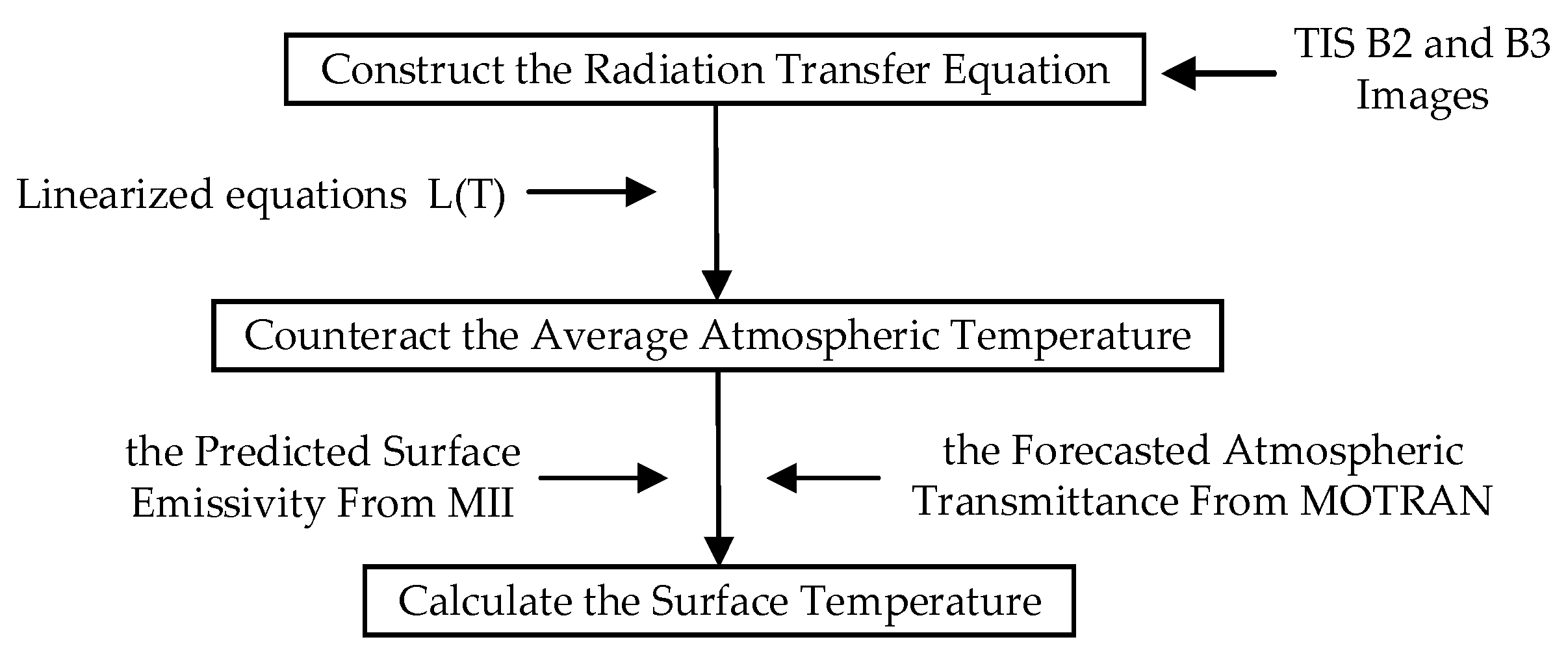
SST retrieval is one of the indispensable steps in the study of thermal effluent distribution. In this section, we introduce the conventional RTE, MW, and NLSST algorithms and we propose the SW method based on 30 m TIS thermal infrared RSIs and 10 m MII multi-spectral images of SDGSAT-1, as shown in Figure 1. First, the thermal infrared and multi-spectral cloudless RSIs of the target regions after geometric and radiometric calibration are selected to obtain the corresponding apparent radiance of the RSIs. Second, in accordance with the red and near-infrared (NIR) bands of multi-spectral data, surface emissivity is calculated to distinguish water from land. Then, we determine the atmospheric profile parameters from the weather conditions of the target region at the imaging time. Finally, according to the theory of surface-atmosphere radiative transfer, the SST of target regions is retrieved using the four methods mentioned above.

2.1. Data Preprocess

2.1.1. Geometric Correction

The cloudless images covering the target NPPs should be geometrically corrected based on the ground control points or digital elevation model, and the small geometric positioning error will be helpful for subsequent processing. In this paper, the geometric correction process for the SDGSAT-1 TIS/MII and Landsat-8 TIRS RSIs employed in the experiment had been previously completed [15,33].

2.1.2. Radiometric Calibration

Ground objects at different temperatures are reflected on the obvious gray discrepancy in the infrared images. As shown in Equation (1), the apparent radiance L λ of thermal infrared and multi-spectral images can be calculated by using the calibration coefficients provided by the official website:
L λ = g a i n × D N + b i a s
where gain and bias, respectively, represent the absolute calibration gain and offset, and can be obtained from the meta-files, as shown in Table 3. DN is the gray value of the pixels. The temperature (T) of thermal infrared images can be deduced from Planck’ law [34], as shown in Equation (2):
T = k 2 l n [ k 1 L λ ( T ) + 1 ]
where k1 and k2 are the specific thermal conversion coefficients depending on the wavelength λ ( μ m ) , as shown in Table 3.

2.2. Surface Emissivity Calculation

Surface emissivity ( ε ) is one of the most important parameters in earth surface temperature retrieval [35], which affects the radiation emitted from the Earth’s diverse surface. The emissivity of a surface mainly depends on the material structure of the target surface, the spectral range of the detector, and the pixel resolution. Surface emissivity varies slightly with the wavelength and can be replaced by the surface emissivity at the channel’s central wavelength. Generally, the Earth’s surface can be divided into water, towns, and bare land, and their emissivity can be calculated by using the NDVI threshold method as Equations (3)–(5) [13,36]. The spectral characteristics of water are obviously distinct from others, whose surface emissivity can be estimated as 0.995 in surface temperature retrieval (8–12 μm). Compared to land surface temperature retrieval, water pixels account for a larger proportion in SST retrieval. Water-land separation is employed in SST retrieval to independently retrieve the water surface temperature. For areas that are easily affected by tides, the NDVI threshold method is often used for water-land separation. For areas that are not easily affected by tides, the water surface can be directly extracted according to fixed shoreline boundaries.
{ ε w a t e r = 0.995 ε t o w n s = 0.9589 + 0.086 × F v 0.0671 × F v × F v ε b a r e - l a n d = 0.9625 + 0.0614 × F v 0.0461 × F v × F v
F v = [ N D V I N D V I min N D V I N D V I max ] 2
N D V I = P ( Re d ) P ( N I R ) P ( Re d ) + P ( N I R )
where F v is the fractional vegetation. NDVI is the normalized difference vegetation index and can be deduced from Equation (5). N D V I min / max is the minimum/maximum of NDVI in the target region, which represents the pure soil/vegetation. Generally, N D V I min = 0.05 and N D V I max = 0.7 . P is the pixel value of the radiometric calibrated red/NIR images and can be calculated using Equation (1).

2.3. Atmospheric Transmissivity Calculation

Atmospheric transmissivity, which is affected by fluctuations in meteorological conditions such as atmospheric pressure, humidity, and gas density, can change significantly, and therefore, can have an obvious impact on infrared radiation transmission [37] and the accuracy of SST retrieval. In view of the difficulties in obtaining real-time atmospheric profile data, researchers have typically used MODTRAN, LOWTRAN, 6S, and other software to simulate atmospheric transmittance τ [37]. For the MODIS, NIR images (B2/B19) can be used to retrieve atmospheric water vapor content w ( g / c m 2 ) ; thus, some researchers haved also estimated τ by simulating the relationship between w and the band-31/32 atmospheric transmissivity τ 31 / 32 , as shown in Equations (6) and (7) [38]:
w = [ 0.02 ln ( r e f 19 / r e f 2 ) ] / 0.651
{ τ 31 = 5.72 4.69 e w / 42.05 , R 2 = 1.00 τ 31 = 1.25 + 2.28 e w / 12.44 , R 2 = 0.99
where r e f 19 / 2 is the band-19/2 surface emissivity of MODIS.

2.4. SST Retrieval

In the process of surface-atmosphere radiative transfer [39], the thermal energy mainly radiates outward through two atmospheric windows: 3–5 µm and 8–14 µm [40]. The energy received by a thermal infrared sensor includes three parts: the surface heat radiation after atmospheric weakening, the upward atmospheric radiation received by the sensor, and the surface-reflecting energy of the downward atmospheric radiation. Therefore, the apparent radiance of RSIs is inevitably affected by surface temperature, surface emissivity, and atmospheric transmission. Due to the influence of atmospheric absorption (especially, water and gas absorption) and scattering, the total radiation received by the sensor does not reflect the true radiation of the Earth’s surface, and therefore, atmospheric correction is used to eliminate these radiation errors. It is necessary for SST retrieval to remove the atmospheric radiation from thermal infrared RSIs to obtain the real reflectance, radiation, and temperature of the surface. Surface temperature retrieval is essentially a type of special atmospheric correction.

2.4.1. RTE Algorithm

Considering the various atmospheric influences, the RTE method is the most comprehensive and rational algorithm. Assuming that there is uniform atmosphere without cloud interference, when the actual surface temperature is T S (K), the top atmospheric radiation obtained by the thermal infrared imager is the apparent radiance L λ , which is composed of the upward atmospheric radiance L λ a t m , the energy ε λ τ λ L λ ( T S ) from the actual ground radiance passing through the atmosphere and finally reaching the detector, and the reflected energy of the downward radiance ( 1 ε λ ) τ λ L λ a t m . The corresponding blackbody radiation L λ ( T S ) of the object is as shown in Equation (8) and the actual surface temperature T S can be obtained by using Equation (2):
L λ ( T S ) = L λ L λ a t m ε λ τ λ ( 1 ε λ ) L λ a t m ε λ
where ε λ is the surface emissivity and τ λ is the atmospheric transmissivity. L λ a t m is the downward atmospheric radiance. In order to obtain the actual surface temperature T S by employing the RTE algorithm, the surface specific emissivity ε λ , atmospheric transmittance τ λ , L λ a t m , and L λ a t m should be estimated in advance. The abovementioned atmospheric parameters can be simulated in MODTRAN if the air temperature, pressure, relative humidity, elevation, and other meteorological data are known.

2.4.2. MW Algorithm

The MW algorithm can avoid calculation of the upward and downward atmospheric radiation, according to Qin [27]. The calculation formula of the MW algorithm is shown as Equation (9):
T S = { a ( 1 C D ) + T s e n s o r [ b ( 1 C D ) + C + D ] D T a v e } / C
where T S is the actual surface temperature (K). Tsensor is the brightness temperature, which can be obtained by Equation (2). The coefficients a and b should be modified according to the spectral response function if the spectrum changes. When 0 ° C T S 70 ° C , a = 66.2795 , a = 66.2795 and b = 0.4461 for Landsat-8 TIRS band-10 (10.60~11.19 µm) RSIs. C = ε λ τ λ , D = ( 1 τ λ ) [ 1 + ( 1 ε λ ) τ λ ] are the intermediate variables. ε λ is the surface emissivity and τ λ is the atmospheric transmissivity. T a v e is the average atmospheric temperature (K), which can be divided into three cases: tropic, summer in mid-latitudes, and winter in mid-latitudes, as shown in Equation (10). The temperature near the ground ( T 0 ) is usually replaced by the brightness temperature. The MW algorithm needs to calculate the brightness temperature (Tsensor), surface emissivity ( ε λ ), and atmospheric transmissivity ( τ λ ) to obtain the actual surface temperature T S :
{ T a v e - s u m m e r = 16.0110 + 0.92621 T 0 T a v e - wint e r = 19.2704 + 0.91118 T 0 T t r o p i c = 17.9769 + 0.91715 T 0

2.4.3. SW Algorithm

The split-window algorithm, applied mainly for AVHRR SST retrieval, can correct the atmospheric radiation through the combination of two adjacent thermal infrared channels with obviously different atmospheric absorption [41,42]. Currently, there are nearly twenty publicly published split-window algorithms and their basic form is shown as Equation (11), representing surface temperature through a linear/nonlinear combination of brightness temperatures in multiple bands [16]:
T S = A 0 + A 1 T i + A 2 T j
where T S (K) is the actual surface temperature; T i , T j are, respectively, the brightness temperature of band-i and band-j; A 0 , A 1 , A 2 are the parameters determined by the atmospheric transmissivity and surface emissivity.
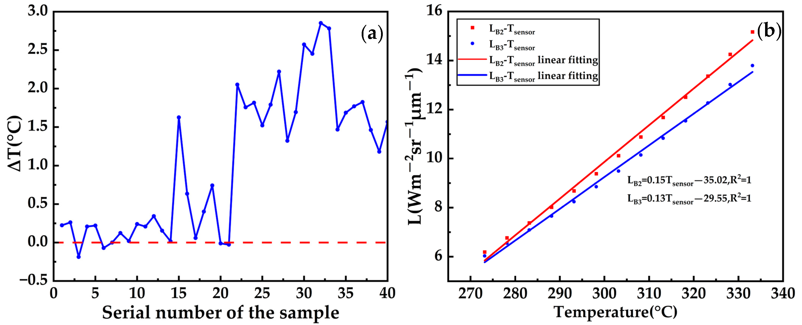
SDGSAT-1 TIS, containing three thermal infrared bands with a spatial resolution of 30 m, has the advantages of more thermal channels and higher spatial resolution which is suitable for surface temperature retrieval in the offshore sea. The brightness temperature difference between TIS B2 and B3 of forty samples are calculated by using Equations (1) and (2). As shown in Figure 2a, there are seven samples less than zero and thirty-three samples greater than zero. It is obvious that the radiation of the two adjacent bands is actually different. In this paper, we select the TIS B2 images as the data source for the RTE and MW algorithms and take the combination of the TIS B2 and B3 images as the input for the SW and NLSST algorithms.
The SW algorithm that is suitable for SDGSAT-1 images is derived as shown in Figure 3, which needs fewer parameters and facilitates its quantitative application by counteracting the average atmospheric temperature.
First, we construct the radiative transfer equation for TIS B2 and B3 images as Equation (12).
{ L 2 ( T 2 ) = ε τ 2 ( θ ) L 2 ( T S ) + [ 1 τ 2 ( θ ) ] × [ 1 + ( 1 ε ) τ 2 ( θ ) ] L 2 ( T T ) L 3 ( T 3 ) = ε τ 3 ( θ ) L 3 ( T S ) + [ 1 τ 3 ( θ ) ] × [ 1 + ( 1 ε ) τ 3 ( θ ) ] L 3 ( T T )
where T 2 , T 3 (K) are the brightness temperature of the TIS B2 and B3 RSIs, respectively. T S (K) is the actual surface temperature and T T (K) is the average atmospheric temperature. ε is the surface emissivity (8–12 μm) and τ 2 ( θ ) , τ 3 ( θ ) are the atmospheric transmissivity when the zenith angle of TIS is θ . L 2 ( T 2 ) , L 3 ( T 3 ) are the apparent radiance received by the sensor and L 2 ( T T ) , L 3 ( T T ) are the apparent radiance corresponding to the average atmospheric temperature. It is difficult to directly calculate the surface temperature because of the complex nonlinear properties of the Planck equation [34]. We provide the scatter plot between temperature and apparent radiance based on the TIS B2 and B3 images, as shown in Figure 2b. It is found that the relationship between temperature and apparent radiance is approximately linear in 0–50 °C, as Equation (13). Then, Equation (12) can be reduced to Equation (14) by counteracting T T . Finally, T S can be estimated only if ε and τ 2 ( θ ) , τ 3 ( θ ) are predicted according to Section 2.2 and Section 2.3.
{ L 2 = a 2 T b 2 = 0.15 T 35.02 , R 2 = 1 L 3 = a 3 T b 3 = 0.13 T 29.55 , R 2 = 1
T s = M 3 M 2 ( b 2 a 2 b 3 a 3 ) + M 3 ( a 2 T 2 b 2 ) M 2 ( a 3 T 3 b 3 ) + P b 2 Q b 3 ( P a 2 Q a 3 )
{ M 3 = { a 3 ( 1 τ 3 ) [ 1 + τ 3 ( 1 ε ) ] } M 2 = { a 2 ( 1 τ 2 ) [ 1 + τ 2 ( 1 ε ) ] } P = M 3 τ 2 ε Q = M 2 τ 3 ε
where a 2 = 0.15 , b 2 = 35.02 , a 3 = 0.13 , b 3 = 29.55 and M 2 , M 3 , P , Q are the intermediate parameters determined by the atmospheric transmissivity and surface emissivity.

2.4.4. NLSST Algorithm

The relative spectral response functions for different channels of the TIS, AVHRR, MODIS, and TIRS sensors are shown in Figure 4 and the setting of the two thermal infrared bands (B2: 10.30–11.3 μm and B3:11.5–12.5 μm) of SDGSAT-1 TIS is consistent with the CH4 (10.30–11.3 μm) and CH5 (11.5–12.5 μm) of NOAA AVHRR, as shown in Table 1 and Table 2. The NLSST algorithm is specially designed for AVHHR CH4 and CH5. The SST results retrieved from the SSW algorithm should be theoretically similar to those of the NLSST algorithm for the same RSIs.
Here, we take the NLSST algorithm [12] as a contrast to evaluate the accuracy of the SW algorithm, as Equation (16):
T S = C 1 T 4 + C 2 ( T 4 T 5 ) + C 3 ( T 4 T 5 ) ( s e c θ 1 ) + C 4
where T S (K) is the actual surface temperature and T 4 , T 5 are the brightness temperature (K) of the AVHRR CH4 and CH5 RSIs, respectively. θ is the zenith angle of the sensor. c 1 = 1.0222 , c 2 = 2.31 , c 3 = 0.83 , c 4 = 280.39 , which are regressed by the drifting and fixed buoys data in the tropical Pacific.

3. Results and Discussion

3.1. Experimental Data

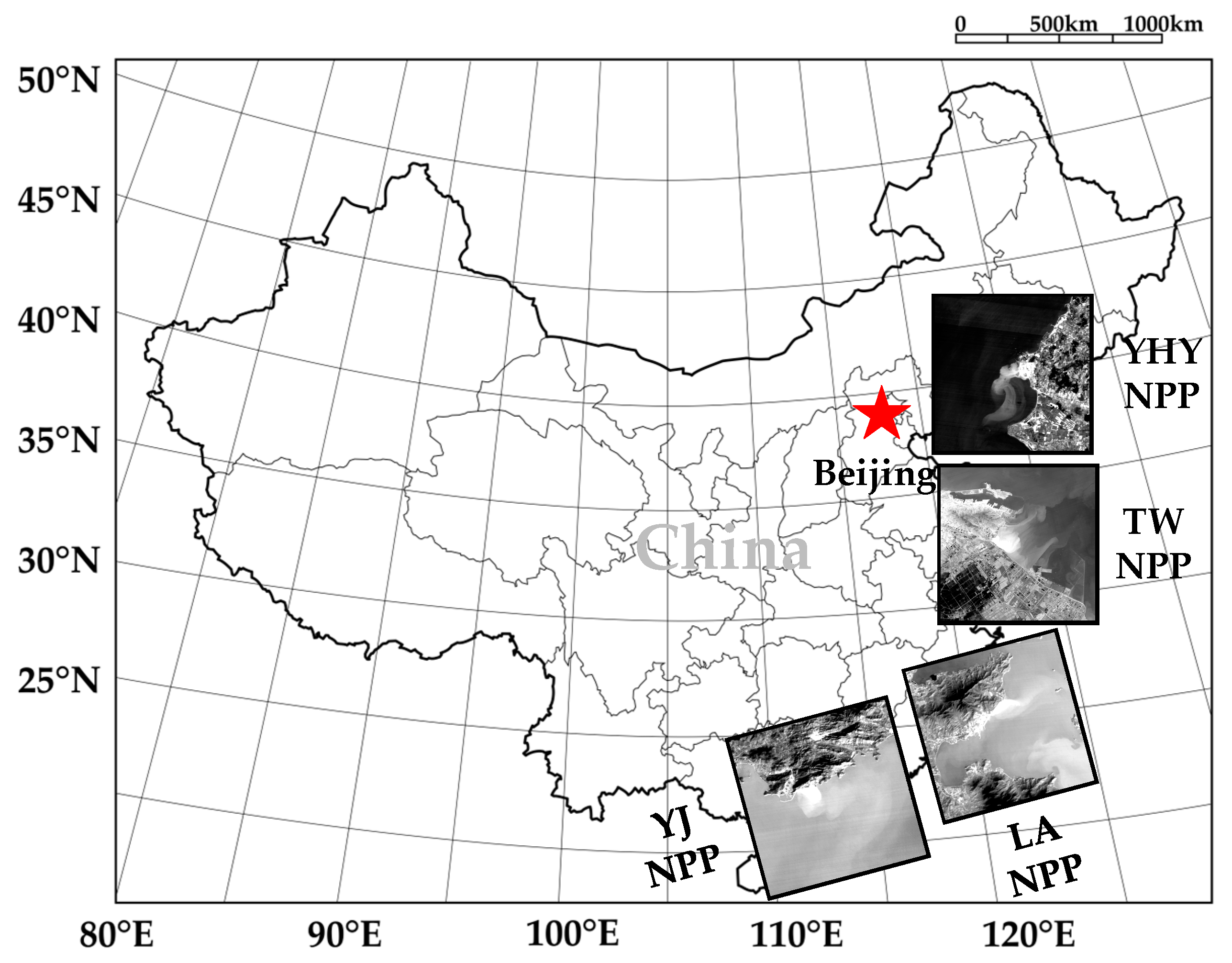
In this study, the Tianwan (TW), Ling’ao (LA), Yangjiang (YJ), and Hongyan River (HY) NPPs and their adjacent sea areas are taken as our experimental areas, and their geographical distribution is shown in Figure 5. The TW NPP, located in Lianyungang City, Jiangsu Province, is the largest single capacity NPP which can accommodate eight nuclear power generation units in the order of megawatts with a total installed capacity of 8–10 million kilowatts and an annual power generation of 60–70 billion kilowatt hours. The LA NPP is China’s first large commercial NPP with a total of six megawatt class pressurized water reactor nuclear power units, located in Dapeng New District, Shenzhen City, Guangdong Province. It has an annual generating capacity of about 45 billion kilowatt hours. The YJ NPP, located in Dongping Town, Yangjiang City, Guangdong Province, is the only private NPP in southern China with a total installed capacity of 1100 megawatts. The HY NPP, located in Hongyan River Town, Wafangdian City, Liaoning Province, is the first NPP in northeast China with a total of six million kilowatts pressurized water reactor nuclear power units.
Eighteen TIS images and thirteen MII images, with less than 5% cloud cover, of the four NPPs are selected and the corresponding Landsat-8 TIRS images in the same place are picked out as the contrast. The images’ detailed information is shown in Table 4 and all the experimental images have been geometric corrected and cropped to the same size (1000 pixels × 1000 pixels). ‘Image Name’ in Table 4 is in the form ‘NPP-sensor-time’. ‘TW-TIS-220517’ represents the TIS image of the Tianwan Nuclear Power Plant taken on 17 May 2022.

3.2. Results and Discussion

In this paper, twenty-two thermal infrared RSIs that originated from the TIS/TIRS at the TW, LA, YJ, and HY NPPs are selected to quantitatively retrieve SST. As shown in Figure 1, first, we crop the selected images to obtain experimental images that fully cover the potential temperature rising area. Then, four SST retrieval algorithms (RTE, MW, NLSST, and SW) are employed to retrieve SST. Next, we grade the SST distribution and mark the temperature rise levels with different colors. Finally, we count the distribution acreage at every level.
The SST that is not affected by thermal pollution is called the datum T 0 . Objective and accurate T 0 is of great significance for evaluating the thermal contamination of NPPs and methods for obtaining T0 must avoid the influence of potential thermal discharge. Additionally, T0 should represent the average temperature in the measurement area at different times as much as possible. For open seas, SST in the same area before the NPPs’ operation can be taken as T 0 . For semi-closed seas, the average SST of the area not polluted by thermal discharge can be used as T 0 . In this experiment, all four NPPs are semi-closed seas and the average SST of the area away from temperature rising area is defined as datum T 0 . After obtaining the SST and datum T 0 , the temperature rising area is determined. In this paper, we formulate the specification and mapping for temperature rise levels, as shown in Table 5, and different colors are used to mark the temperature rise levels. According to the number of pixels occupied by each temperature rising level and the spatial resolution of RSIs, the distribution acreage and area proportions of different temperature rise levels can be derived.

3.2.1. SST Distribution

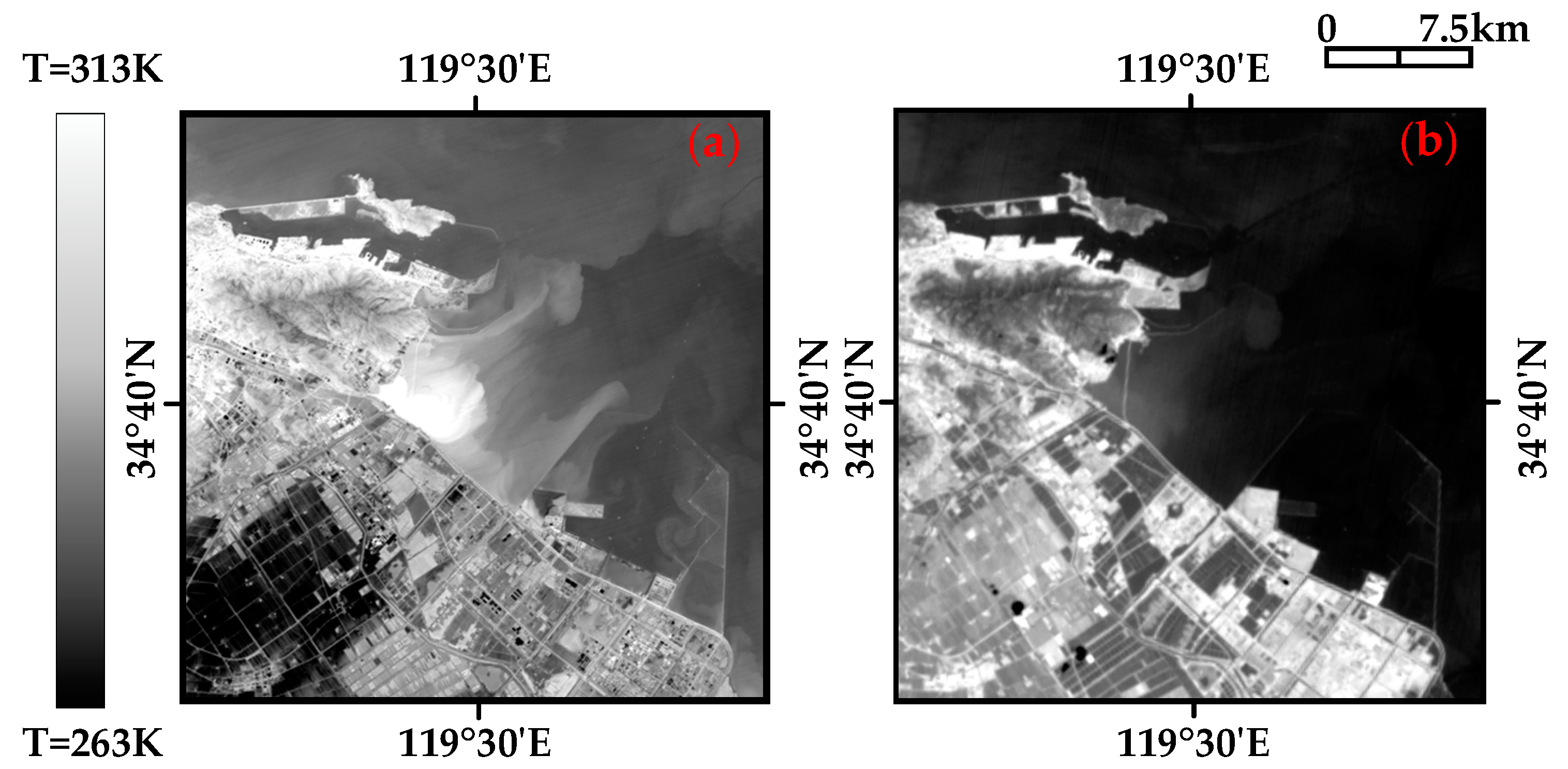
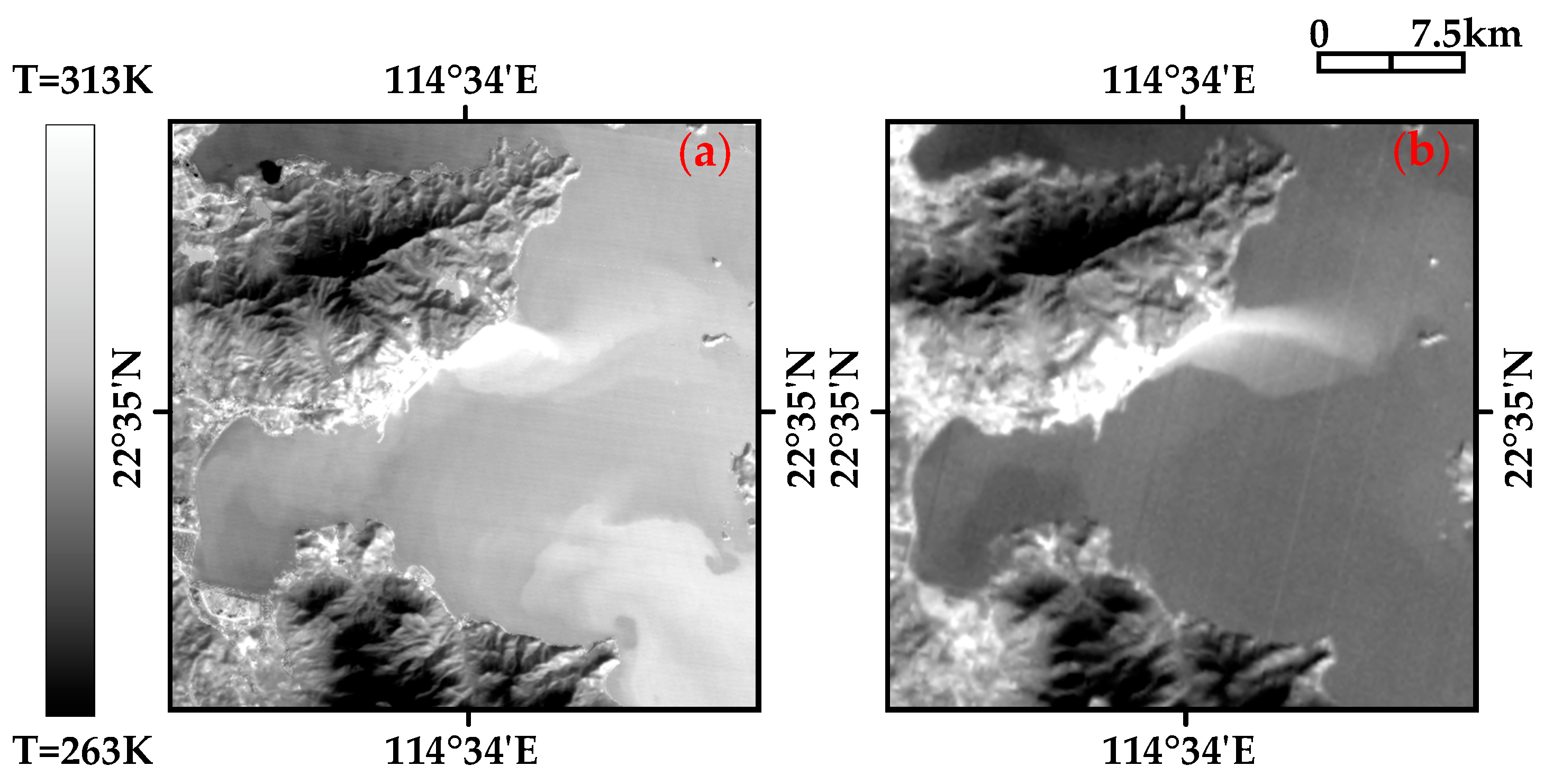
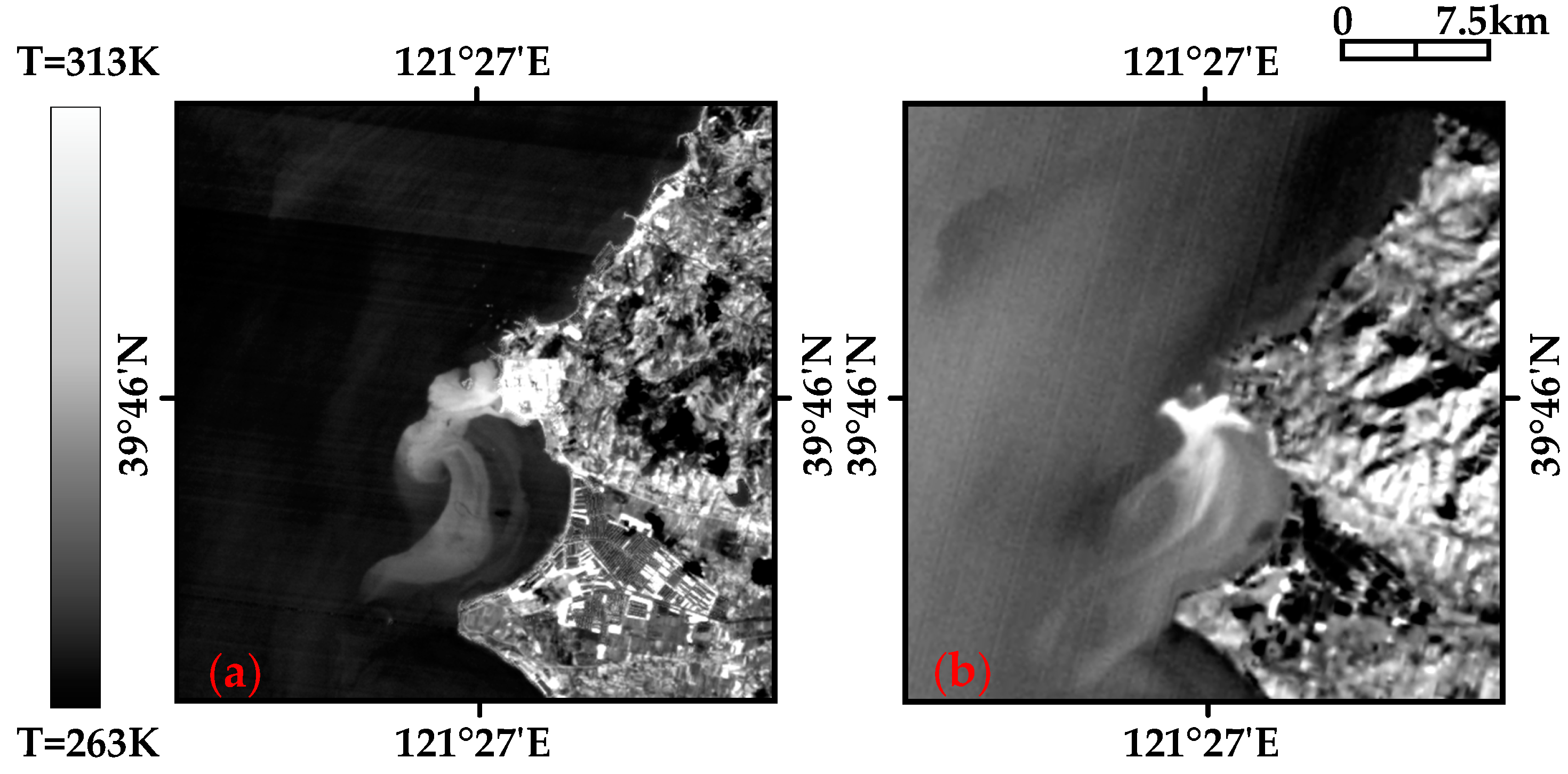
The SST retrieved from the SDGSAT-1 TIS and Landsat-8 TIRS images of the TW NPP, LA NPP, YJ NPP, and HY NPP are, respectively, displayed in Figure 6, Figure 7, Figure 8 and Figure 9. It is obvious that the TIS images can depict more prominent boundary and clearer details than TIRS images because of higher spatial resolution (30 m). Considering that the distribution of thermal discharge is easily influenced by the season, tides, and geographical location, the multi-temporal and higher spatial-resolution TIS data are more suitable for describing the subtle changes in thermal discharge than that of Landsat-8 TIRS, MODIS, and AVHRR data. Therefore, TIS data are a better option for monitoring subtle variations in thermal discharge and for evaluating marine environments.

3.2.2. SST Comparison

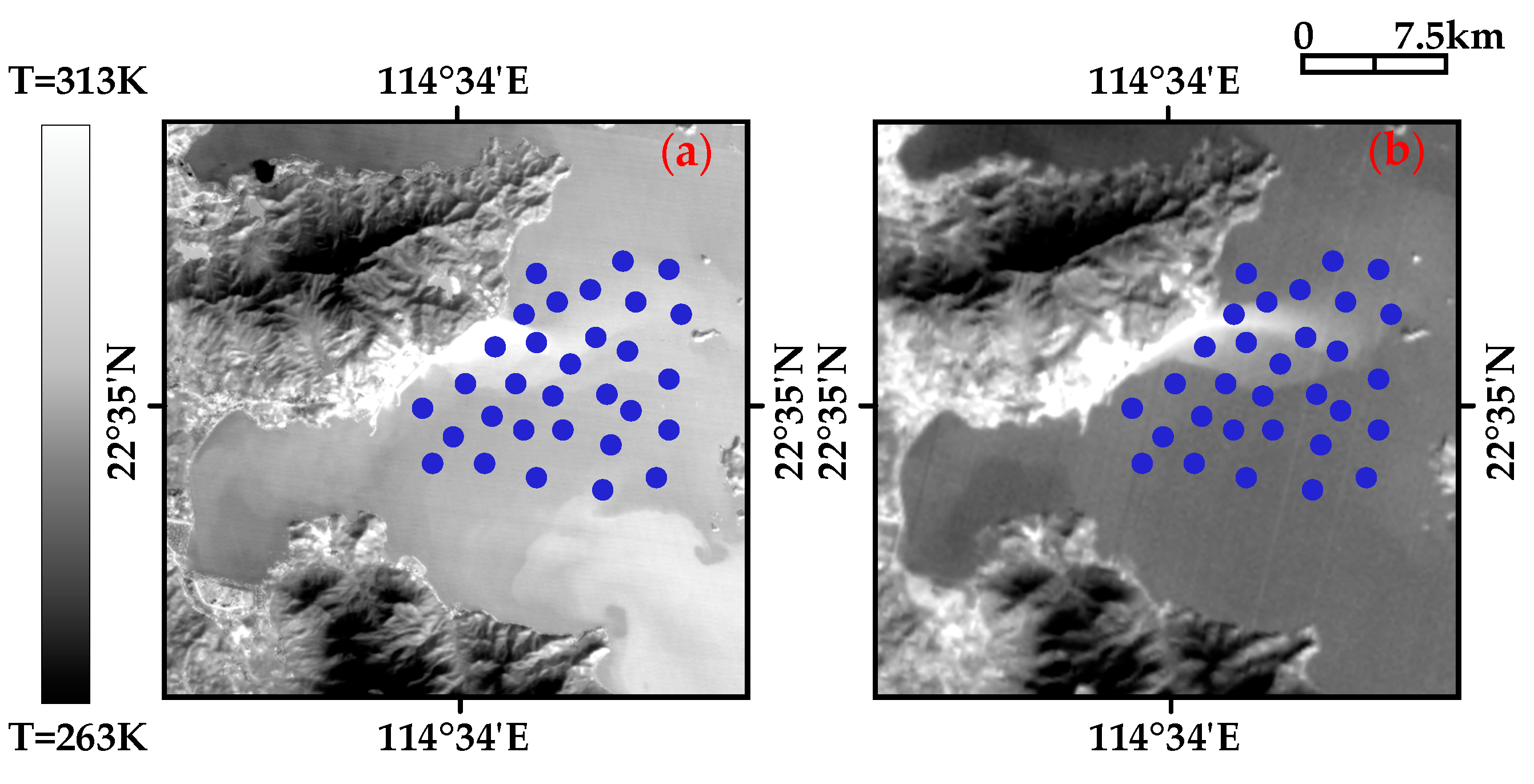
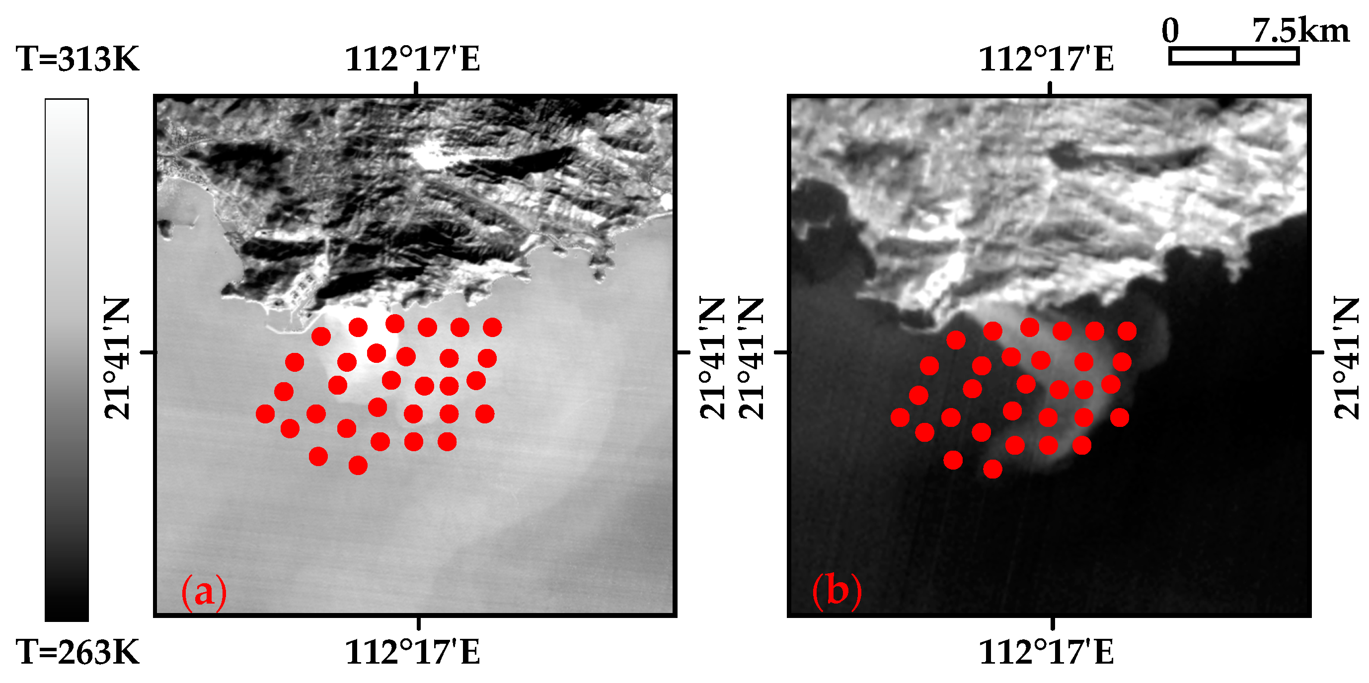
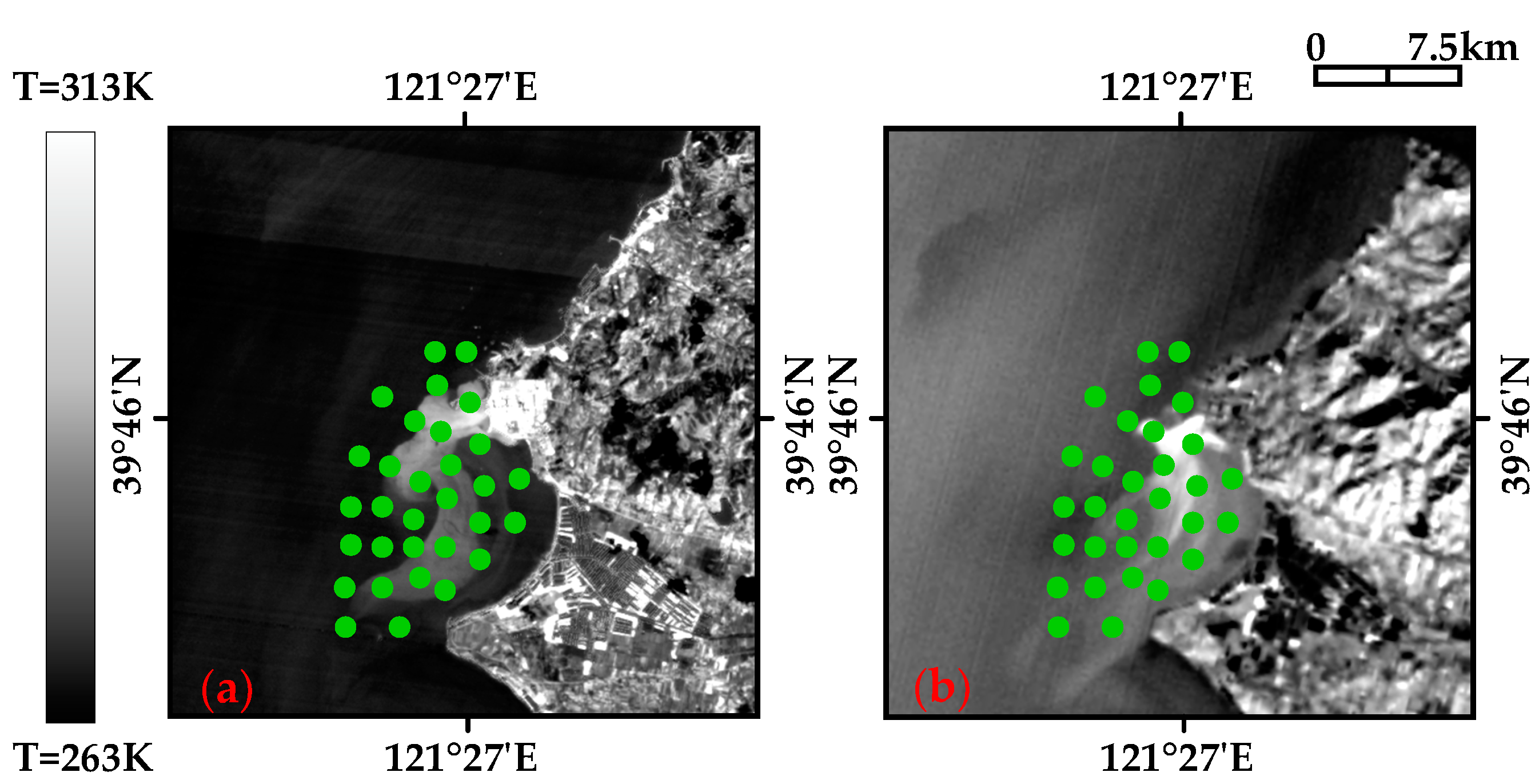
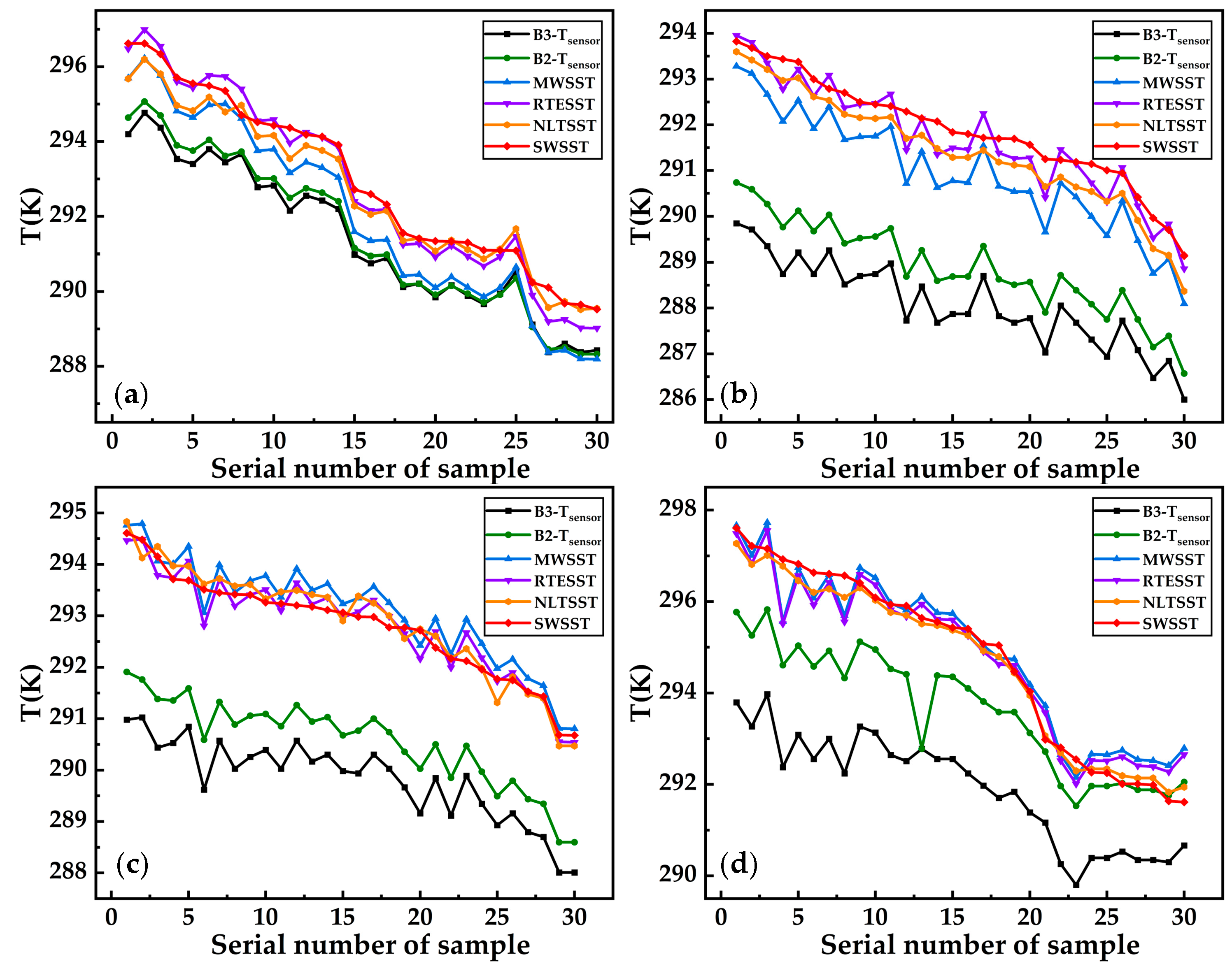
In Figure 10, Figure 11, Figure 12 and Figure 13, thirty-one points are uniformly sampled from the SST results retrieved from the TW NPP, LA NPP, YJ NPP, and HY NPP TIS images, respectively. The brightness temperature of B2 (B2-Tsensor), brightness temperature of B3 (B3-Tsensor), SST retrieved by the MW algorithm (MWSST), SST retrieved by the RTE algorithm (RTESST), SST retrieved by the NLSST algorithm (NLSST), and SST retrieved by the SW algorithm (SWSST) of the 31 sampling points are statistically shown in Figure 14.
The Experimental results show the following:
(1)
MWSST, RTESST, NLSST, and SWSST are all higher than B2/B3-Tsensor by about 3–5 °C.
(2)
The SST retrieved from the split-window algorithms (SWSST and NLSST) is generally higher than that of the single-channel algorithms (MWSST and RTESST), which is largely related to the fact that the split-window algorithms can correct atmospheric effect and obtain more accurate SST.
(3)
The values of SWSST and NLSST are close to each other, with a small difference of 0.5 °C. It is inferred that the small difference is relevant to the NLSST algorithm’s empirical coefficients, which have not been updated for a long time. The small difference also confirms the theoretical hypothesis stated in Section 2.4.4, which relatively verifies the accuracy of the SW algorithm.

3.2.3. Thermal Discharge Monitoring

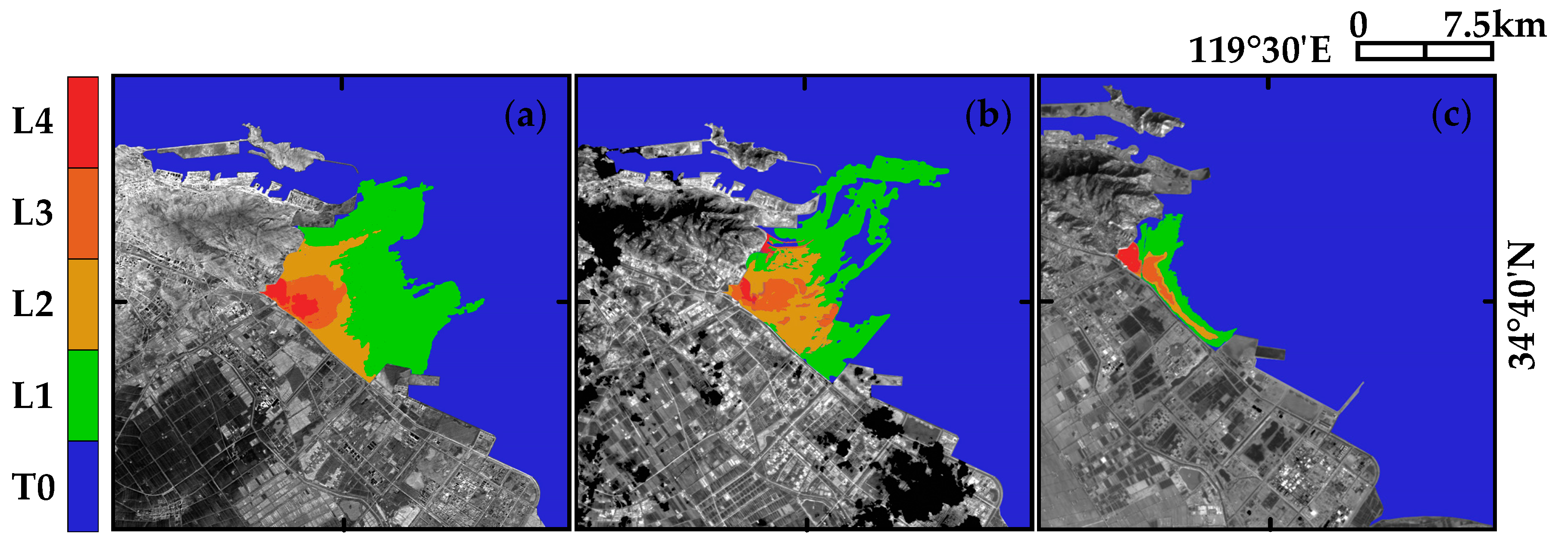
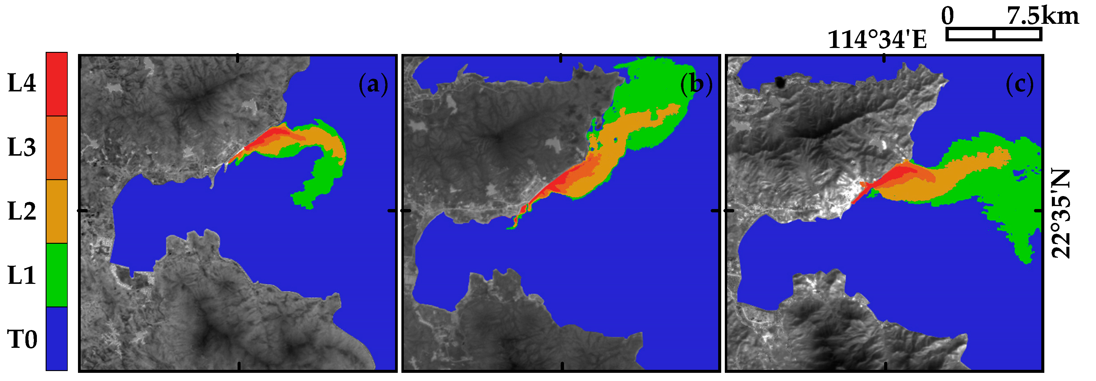
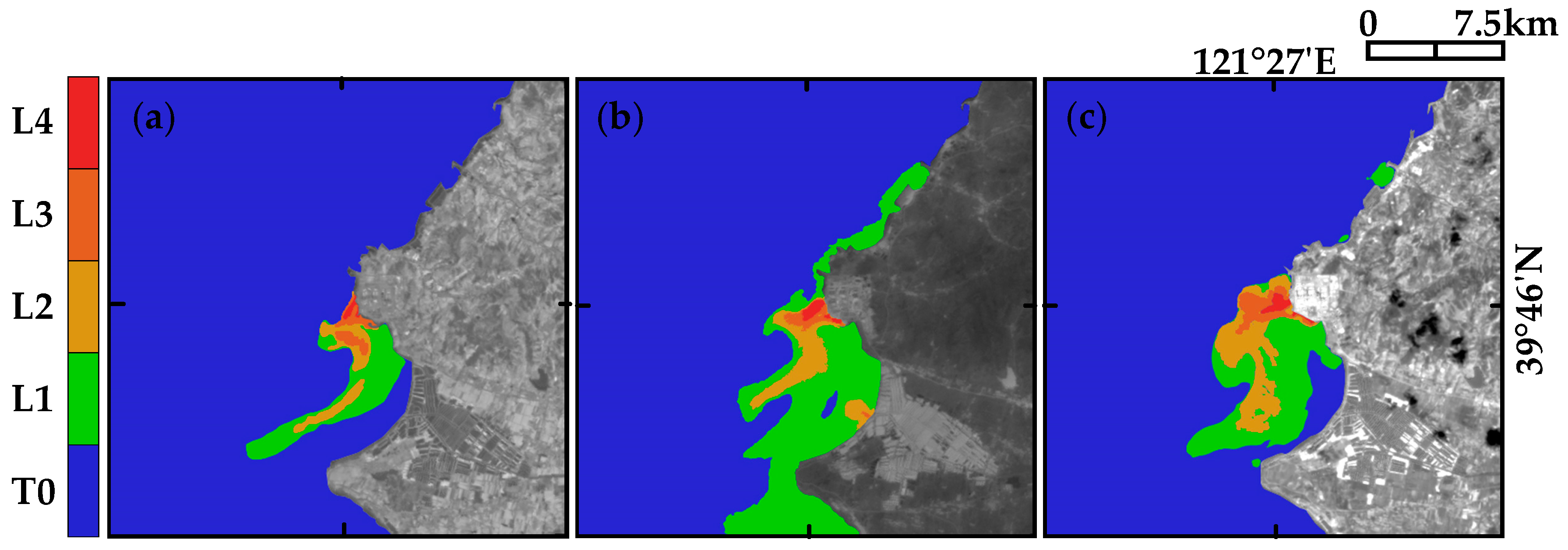
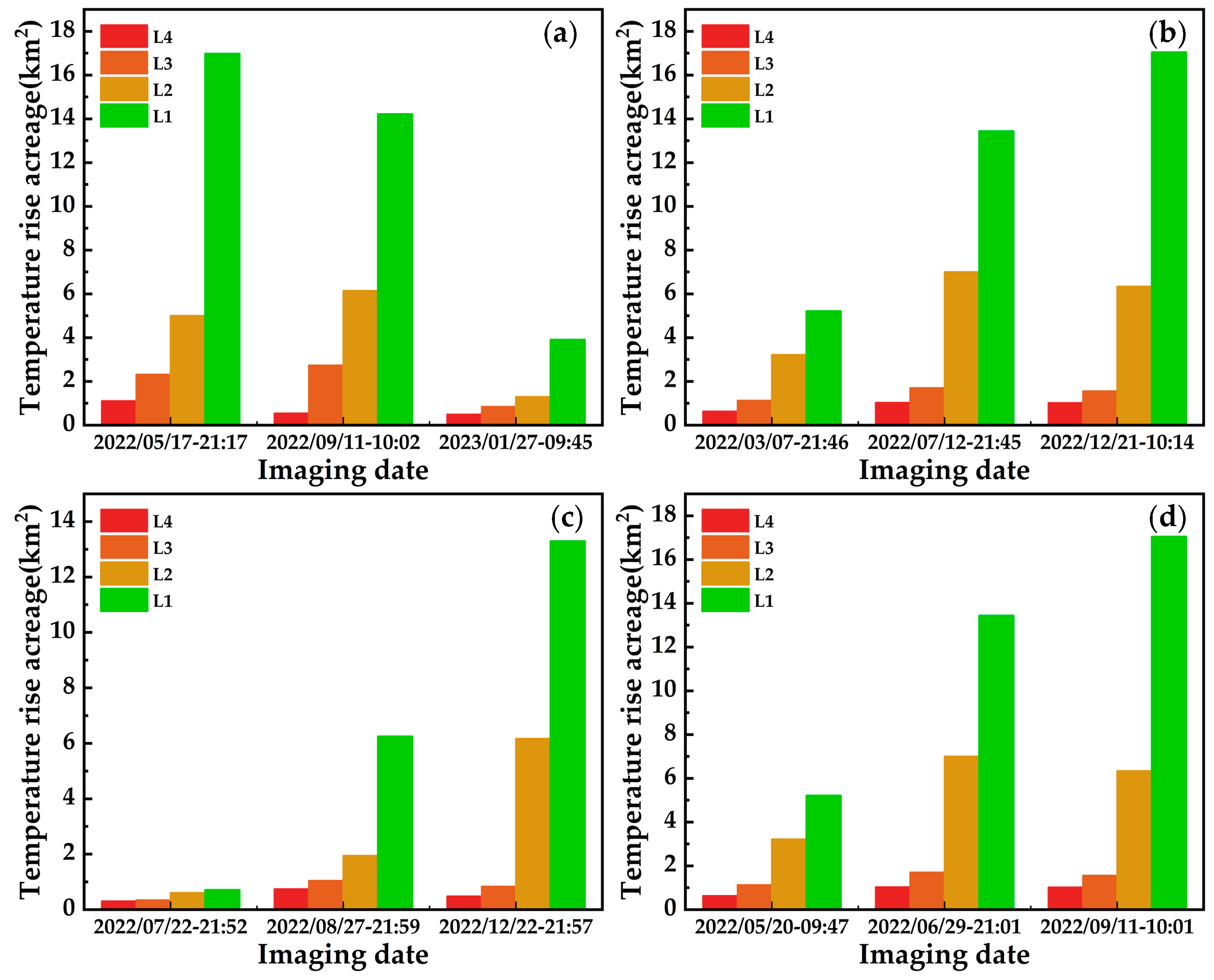
As shown in Figure 15, Figure 16, Figure 17 and Figure 18, five different colors are used to mark the temperature rise levels retrieved from the TW NPP, LA NPP, YJ NPP, and HY NPP TIS images under different months. Afterwards, the number of pixels and the acreage occupied by different temperature rise levels are calculated (the corresponding acreage of a single pixel is 30 m × 30 m). As shown in Figure 19, the statistical analysis shows that:
(1)
Obvious seasonal variation of the temperature rise area is monitored near the outfall of the four NPPs. The proportion of L1 temperature rise area is the largest (about 15 km2 in winter and 5 km2 in summer) and the smallest proportion is the L4 area (about 2 km2 in winter and 0.5 km2 in summer).
(2)
The highest temperature difference is about 4 °C, and the total acreage of temperature rise area is about 25 km2, diffusing in a feather-shape to distant natural seas.
(3)
The temperature rise areas of different NPPs have obvious distinctions influenced by terrain, climate, wind direction, tides, and geographical location.

4. Conclusions

In this paper, we propose a simplified split-window-based temperature retrieval method (SW method) that is suitable for SDGSAT-1 TIS RSIs and which needs only atmospheric transmissivity and surface emissivity by counteracting the average atmospheric temperature. We quantitatively retrieve the SST of the TW NPP, LA NPP, YJ NPP, and HY NPP with thermal infrared RSIs from the SDGSAT-1 TIS and Landsat-8 TIRS. The TIS images (30 m) can depict more prominent boundary and clearer details than the TIRS images (100 m) because of higher spatial resolution. The SST retrieved from the split-window algorithms (SSWSST and NLSST) is generally higher than that of the single-channel algorithms (MWSST and RTESST), which is largely related to the fact that the split-window algorithms can correct atmospheric effect and obtain more accurate SST. The obvious seasonal variations in the temperature rise area are monitored near the outfall of the four NPPs. Through the above research, we find that the SDGSAT-1 TIS images can better describe the detailed distribution of thermal discharge based on the SW method, which provides a feasible and efficient method to monitor thermal pollution in small-scale regions. However, there are some uncertain factors in the retrieval process, including water and gas absorption, cloud coverage, mixed pixels, and proximity effect, which may cause some deviations in the retrieval results. Preprocessing of thin clouds can restore real surface information and reduce retrieval errors, which is an essential link in remote sensing analysis and application. Therefore, accurate atmospheric correction and cloud detection preprocessing are also important steps in the future optimization of thermal discharge monitoring.

Author Contributions

Conceptualization, W.H. and X.P.; methodology, W.H.; software, W.H. and L.Y.; validation, X.P. and W.H.; formal analysis, W.H.; investigation, W.H. and L.Z.; resources, F.C. and. X.L.; data curation, Z.H. and X.L.; writing—original draft preparation, W.H.; writing—review and editing, W.H. and J.J.; visualization, W.H.; supervision, Z.H. and X.L.; project administration, F.C.; funding acquisition, F.C. All authors have read and agreed to the published version of the manuscript.

Funding

This research was funded by the Strategic Priority Research Program of the Chinese Academy of Sciences, grant number XDA19010102, and the National Natural Science Foundation of China under grant number 61975222.

Data Availability Statement

Not applicable.

Acknowledgments

The authors would like to thank the SDG BIGDATA Center and National Space Science Center for providing us with data.

Conflicts of Interest

The authors declare no conflict of interest.

References

  1. Gaeta, M.G.; Samaras, A.G.; Archetti, R. Numerical investigation of thermal discharge to coastal areas: A case study in South Italy. Environ. Model. Softw. 2020, 124, 104596. [Google Scholar] [CrossRef]
  2. Donlon, C.; Minnett, P.; Gentemann, C.; Nightingale, T.; Barton, I.; Ward, B.; Murray, M. Toward improved validation of satellite sea surface skin temperature measurements for climate research. J. Clim. 2002, 15, 353–369. [Google Scholar] [CrossRef]
  3. Schluessel, P.; Emery, W.J.; Grassl, H.; Mammen, T. On the bulk-skin temperature difference and its impact on satellite remote sensing of sea surface temperature. J. Geophys. Res. Ocean. 1990, 95, 13341–13356. [Google Scholar] [CrossRef]
  4. Fox-Kemper, B.; Hewitt, H.; Xiao, C.; Aðalgeirsdóttir, G.; Drijfhout, S.; Edwards, T.; Golledge, N.; Hemer, M.; Kopp, R.; Krinner, G. Ocean, cryosphere and sea level change. AGU Fall Meet. Abstr. 2021, 2021, U13B-09. [Google Scholar]
  5. Zhang, Z.; Wang, D.; Cheng, Y.; Gong, F. Long-term changes and factors that influence changes in thermal discharge from nuclear power plants in Daya Bay, China. Remote Sens. 2022, 14, 763. [Google Scholar] [CrossRef]
  6. Wang, X.; Gong, C.; Hu, Y.; Wang, X.; Li, L.; He, Z. Retrieval of sea surface temperature and thermal discharge monitoring in nuclear power plant using Gaofen-5 satellite remote sensing imagery. J. Appl. Remote Sens. 2022, 16, 012013. [Google Scholar] [CrossRef]
  7. Tang, D.; Kester, D.R.; Wang, Z.; Lian, J.; Kawamura, H. AVHRR satellite remote sensing and shipboard measurements of the thermal plume from the Daya Bay, nuclear power station, China. Remote Sens. Environ. 2003, 84, 506–515. [Google Scholar] [CrossRef]
  8. Chen, C.; Shi, P.; Mao, Q. Application of remote sensing techniques for monitoring the thermal pollution of cooling-water discharge from nuclear power plant. J. Environ. Sci. Health Part A 2003, 38, 1659–1668. [Google Scholar] [CrossRef]
  9. Chelton, D.B.; Wentz, F.J. Global microwave satellite observations of sea surface temperature for numerical weather prediction and climate research. Bull. Am. Meteorol. Soc. 2005, 86, 1097–1116. [Google Scholar] [CrossRef]
  10. Minnett, P.J.; Barton, I.J. Remote sensing of the earth’s surface temperature. Radiom. Temp. Meas. Ii Appl. 2010, 43, 333–391. [Google Scholar]
  11. Szczodrak, M.D.; Minnett, P.J. Relative Merits of Optimal Estimation and Non-Linear Retrievals of Sea-Surface Temperature from MODIS. Remote Sens. 2022, 14, 2249. [Google Scholar] [CrossRef]
  12. Walton, C.C. Nonlinear multichannel algorithms for estimating sea surface temperature with AVHRR satellite data. J. Appl. Meteorol. Climatol. 1988, 27, 115–124. [Google Scholar] [CrossRef]
  13. Dash, P.; Göttsche, F.-M.; Olesen, F.-S.; Fischer, H. Separating surface emissivity and temperature using two-channel spectral indices and emissivity composites and comparison with a vegetation fraction method. Remote Sens. Environ. 2005, 96, 1–17. [Google Scholar] [CrossRef]
  14. Nie, P.; Zhu, H.; Xu, H.; Huang, Y.; Hua, W. Monitoring of Tianwan Nuclear Power Plant Thermal Pollution Based on Remotely Sensed Landsat Data. In Proceedings of the IGARSS 2020-2020 IEEE International Geoscience and Remote Sensing Symposium, Waikoloa, HI, USA, 26 September–2 October 2020; pp. 5624–5627. [Google Scholar]
  15. Zhang, J.; Li, X.; Li, L.; Sun, P.; Su, X.; Hu, T.; Chen, F. Lightweight U-Net for cloud detection of visible and thermal infrared remote sensing images. Opt. Quantum Electron. 2020, 52, 397. [Google Scholar] [CrossRef]
  16. Minnett, P.; Alvera-Azcárate, A.; Chin, T.; Corlett, G.; Gentemann, C.; Karagali, I.; Li, X.; Marsouin, A.; Marullo, S.; Maturi, E. Half a century of satellite remote sensing of sea-surface temperature. Remote Sens. Environ. 2019, 233, 111366. [Google Scholar] [CrossRef]
  17. Wick, G.A.; Jackson, D.L.; Castro, S.L. Assessing the ability of satellite sea surface temperature analyses to resolve spatial variability–The northwest tropical Atlantic ATOMIC region. Remote Sens. Environ. 2023, 284, 113377. [Google Scholar] [CrossRef]
  18. Tanahashi, S.; Kawamura, H.; Matsuura, T.; Takahashi, T.; Yusa, H. Improved estimates of wide-ranging sea surface temperature from GMS S-VISSR data. J. Oceanogr. 2000, 56, 345–358. [Google Scholar] [CrossRef]
  19. Wu, Y.; Tang, F.; Dai, Y.; Wang, F.; Shi, Y.; Zhang, S. Blend with the Sea Surface Temperature from Different Satellites and Their Comparison in the Southeast Pacific Ocean. J. Ocean Univ. China 2023, 22, 452–458. [Google Scholar] [CrossRef]
  20. Merchant, C.J.; Le Borgne, P. Retrieval of sea surface temperature from space, based on modeling of infrared radiative transfer: Capabilities and limitations. J. Atmos. Ocean. Technol. 2004, 21, 1734–1746. [Google Scholar] [CrossRef]
  21. Embury, O.; Merchant, C.J.; Filipiak, M.J. A reprocessing for climate of sea surface temperature from the along-track scanning radiometers: Basis in radiative transfer. Remote Sens. Environ. 2012, 116, 32–46. [Google Scholar] [CrossRef]
  22. Xuejiao, C.; Yunzhi, C. Mono-window Algorithm Applicability in Fujian Sea and Its Surrounding Areas Sea Surface Temperature Retrieval. Remote Sens. Technol. Appl. 2017, 32, 773–779. [Google Scholar]
  23. Jiménez-Muñoz, J.C.; Sobrino, J.A. A generalized single-channel method for retrieving land surface temperature from remote sensing data. J. Geophys. Res. Atmos. 2003, 108, 4688. [Google Scholar] [CrossRef]
  24. Fu, J.; Chen, C.; Guo, B.; Chu, Y.; Zheng, H. A split-window method to retrieving sea surface temperature from Landsat 8 thermal infrared remote sensing data in offshore waters. Estuar. Coast. Shelf Sci. 2020, 236, 106626. [Google Scholar] [CrossRef]
  25. McMillin, L.M. Estimation of sea surface temperatures from two infrared window measurements with different absorption. J. Geophys. Res. 1975, 80, 5113–5117. [Google Scholar] [CrossRef]
  26. McMillin, L.; Crosby, D. Theory and validation of the multiple window sea surface temperature technique. J. Geophys. Res. Ocean. 1984, 89, 3655–3661. [Google Scholar] [CrossRef]
  27. Qin, Z.-H.; Zhang, M.-H.; Karnieli, A.; Berliner, P. Mono-window algorithm for retrieving land surface temperature from Landsat TM6 data. Acta Geogr. Sin. 2001, 56, 456–466. [Google Scholar]
  28. Hanyue, C.; Li, Z.; Jiaguo, L.; Xieyu, F. A comparison of two mono-window algorithms for retrieving sea surface temperature from Landsat8 data in coastal water of Hongyan River nuclear power station. Remote Sens. Nat. Resour. 2018, 30, 45–53. [Google Scholar]
  29. Kleespies, T.J.; McMillin, L.M. Determination of Precipitable Water with the AVHRR (Advanced Very High Resolution Radiometer); Air Force Geophysics Lab Hanscom AFB MA: Bedford, MA, USA, 1988. [Google Scholar]
  30. Hulley, G.C.; Hook, S.J. Generating Consistent Land Surface Temperature and Emissivity Products between ASTER and MODIS Data for Earth Science Research. Geosci. Remote Sens. IEEE Trans. 2011, 49, 1304–1315. [Google Scholar] [CrossRef]
  31. Gillespie, A.; Rokugawa, S.; Matsunaga, T.; Cothern, J.S.; Hook, S.; Kahle, A.B. A temperature and emissivity separation algorithm for Advanced Spaceborne Thermal Emission and Reflection Radiometer (ASTER) images. IEEE Trans. Geosci. Remote Sens. 1998, 36, 1113–1126. [Google Scholar] [CrossRef]
  32. Li, L.; Jiang, L.; Zhang, J.; Wang, S.; Chen, F. A complete YOLO-based ship detection method for thermal infrared remote sensing images under complex backgrounds. Remote Sens. 2022, 14, 1534. [Google Scholar] [CrossRef]
  33. Li, X.; Yang, L.; Su, X.; Hu, Z.; Chen, F. A correction method for thermal deformation positioning error of geostationary optical payloads. IEEE Trans. Geosci. Remote Sens. 2019, 57, 7986–7994. [Google Scholar] [CrossRef]
  34. Planck, M. The Theory of Heat Radiation. 1914. Available online: https://archive.org/details/theoryofheatradi00planrich (accessed on 21 February 2023).
  35. Marcq, S.; Delogu, E.; Chapelier, M.; Vidal, T.H. DirecTES: A Direct Method for Land and Sea Surface Temperature and Emissivity Separation for Thermal Infrared Sensors—Application to TRISHNA and ECOSTRESS. Remote Sens. 2023, 15, 517. [Google Scholar] [CrossRef]
  36. Verdin, J.; Funk, C.; Klaver, R.; Roberts, D. Exploring the correlation between Southern Africa NDVI and Pacific sea surface temperatures: Results for the 1998 maize growing season. Int. J. Remote Sens. 1999, 20, 2117–2124. [Google Scholar] [CrossRef]
  37. Srivastava, A.; Rodriguez, J.F.; Saco, P.M.; Kumari, N.; Yetemen, O. Global Analysis of Atmospheric Transmissivity Using Cloud Cover, Aridity and Flux Network Datasets. Remote Sens. 2021, 13, 1716. [Google Scholar] [CrossRef]
  38. Wan, Z.; Li, Z.-L. A physics-based algorithm for retrieving land-surface emissivity and temperature from EOS/MODIS data. IEEE Trans. Geosci. Remote Sens. 1997, 35, 980–996. [Google Scholar]
  39. Shi, H.; Xiao, Z.; Wen, J.; Wu, S. An Optical–Thermal Surface–Atmosphere Radiative Transfer Model Coupling Framework with Topographic Effects. IEEE Trans. Geosci. Remote Sens. 2020, 60, 1–12. [Google Scholar] [CrossRef]
  40. Zhu, H.; Li, Q.; Zheng, C.; Hong, Y.; Xu, Z.; Wang, H.; Shen, W.; Kaur, S.; Ghosh, P.; Qiu, M. High-temperature infrared camouflage with efficient thermal management. Light Sci. Appl. 2020, 9, 60. [Google Scholar] [CrossRef] [PubMed]
  41. Petrenko, B.; Ignatov, A.; Kihai, Y.; Stroup, J.; Dash, P. Evaluation and selection of SST regression algorithms for JPSS VIIRS. J. Geophys. Res. Atmos. 2014, 119, 4580–4599. [Google Scholar] [CrossRef]
  42. Chen, Y.; Duan, S.-B.; Labed, J.; Li, Z.-L. Development of a split-window algorithm for estimating sea surface temperature from the Chinese Gaofen-5 data. Int. J. Remote Sens. 2019, 40, 1621–1639. [Google Scholar] [CrossRef]
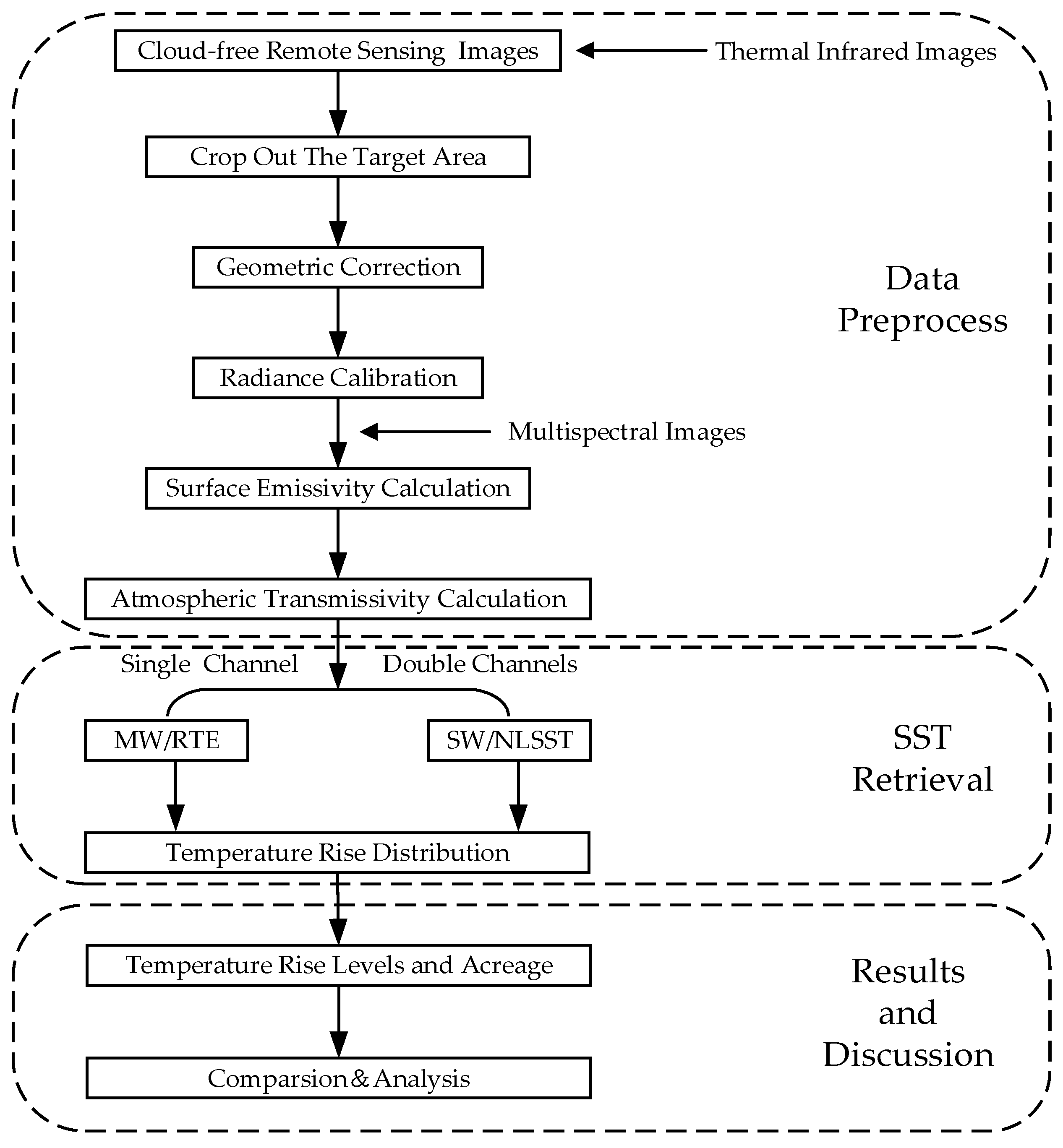
Figure 1. Flowchart of the thermal discharge temperature retrieval and monitoring of the NPPs.
Remotesensing 15 02298 g001
Figure 2. (a) The brightness temperature difference between TIS B2 and B3; (b) the linear fitting between the temperature and radiance for TIS B2 and B3.
Remotesensing 15 02298 g002
Figure 3. Flowchart of the SW algorithm for SDGSAT-1 images.
Remotesensing 15 02298 g003
Figure 4. The relative spectral response function for different channels of the sensors: (a) TIS-B1/B2/B3; (b) AVHRR-CH4/CH5; (c) MODIS-B31/B32; (d) TIRS-B10/B11.
Remotesensing 15 02298 g004
Figure 5. The geographical distribution of the experimental data.
Remotesensing 15 02298 g005
Figure 6. The retrieved SST from the TIS and TIRS images of the TW NPP: (a) TIS; (b) TIRS.
Remotesensing 15 02298 g006
Figure 7. The retrieved SST from the TIS and TIRS images of the LA NPP: (a) TIS; (b) TIRS.
Remotesensing 15 02298 g007
Figure 8. The retrieved SST from the TIS and TIRS images of the YJ NPP: (a) TIS; (b) TIRS.
Remotesensing 15 02298 g008
Figure 9. The retrieved SST from the TIS and TIRS images of the HY NPP: (a) TIS; (b) TIRS.
Remotesensing 15 02298 g009
Figure 10. Spatial distribution of the 31 sampling points from the TW NPP: (a) TIS; (b) TIRS.
Remotesensing 15 02298 g010
Figure 11. Spatial distribution of the 31 sampling points from the LA NPP (a) TIS (b) TIRS.
Remotesensing 15 02298 g011
Figure 12. Spatial distribution of the 31 sampling points from the YJ NPP (a) TIS (b) TIRS.
Remotesensing 15 02298 g012
Figure 13. Spatial distribution of the 31 sampling points from the HY NPP (a) TIS (b) TIRS.
Remotesensing 15 02298 g013
Figure 14. The comparisons of B2/B3 bright temperature, MWSST, RTESST, NLSST, and SWSST of the 31 sampling points around the four NPPs: (a) TW NPP; (b) LA NPP; (c) YJ NPP; (d) HY NPP.
Remotesensing 15 02298 g014
Figure 15. The temperature rise distribution of the TW NPP under different months: (a) 17 May 2022; (b) 11 September 2022; (c) 27 January 2023.
Remotesensing 15 02298 g015
Figure 16. The temperature rise distribution of the LA NPP under different months: (a) 7 March 2022; (b) 12 July 2022; (c) 21 December 2022.
Remotesensing 15 02298 g016
Figure 17. The temperature rise distribution of the YJ NPP under different months: (a) 22 July 2022 (b) 27 August 2022; (c) 11 December 2022.
Remotesensing 15 02298 g017
Figure 18. The temperature rise distribution of the HY NPP under different months: (a) 2 May 2022; (b) 29 June 2022; (c) 11 September 2022.
Remotesensing 15 02298 g018
Figure 19. Column chart of acreage occupied by different temperature rise levels at the four NPPs: (a) TW NPP; (b) LA NPP; (c) YJ NPP; (d) HY NPP.
Remotesensing 15 02298 g019
Table 1. Remote sensing data for SST retrieval.
ItemsPayloadsWavelengthRevisitResolution
MicrowaveFY-3B MWRI10.65/18.7/23.8/36.5/89.0 GHz1 day15–85 km
TRMM TMI10.7/19.4/21.3/37.0/85.5 GHz1–2 days25–50 km
GCOM-W1 AMSR26–89 GHz1–3 days31.25 km
DMSP SSM/I19.36/22.23/37.0/85.5 GHz1 day12.5–25 km
InfraredGOES ABI10.5–12.5 µm0.5–1 h3–10 km
FY2S VISSR10.3–11.3/11.5–12.5 µm
Terra MODIS10.78–11.28/11.77–12.27 µm12 h1 km
NOAA AVHRR10.3–11.3/11.5–12.512 h1.1 km
ERS-2 ATSR-210.35–11.35/11.5–12.5 µm1–2 days1–2 km
FY-3 VIRR10.3–11.3/11.5–12.5 µm1–4 days1.1 km
Sentinel-3 SLSTR10.8–12.02 µm2 days1 km
S-NPP VIIRS8–12 µm16 days750 m
Landsat-7 ETM+10.4–12.5 µm1–16 days100 m
Landsat-8 TIRS10.6–11.19/11.5–12.51 µm16 days
Terra ASTER8.125–8.475/8.475–8.825/8.925–9.275/10.25–10.95/10.95–11.65 µm16 days90 m
Table 2. Technical and performance index of the SDGSAT-1 TIS and MII.
PayloadsSpectrum (μm)Resolution (m)NETD/SNRRadio-Calibration Precision
TISB1:8–10.5300.2 K@300 KRelative: 5%
Absolute: 1 K@300 K
B2:10.30–11.3
B3:11.5–12.5
MIIb1:0.374–0.42710≥130Relative: 2%
Absolute: 5%
b2:0.410–0.467≥150
b3:0.457–0.529
b4:0.510–0.597
b5:0.618–0.696
b6:0.744–0.813
b7:0.798–0.911
Table 3. Parameters for the radiometric calibration of the TIS/MII/TIRS.
ParametersTIS-B1TIS-B2TIS-B3TIRS-B10TIRS-B11MII-RedMII-NIR
gain0.0039470.0039460.0053290.0003420.0003420.0160960.019719
bias0.1671260.1246220.2225300.10.100
k11655.628838.706543.058774.89480.89
k21542.7621342.7191232.0211321.081201.14
Table 4. Detailed information about the selected images.
RegionsImage NameAcquisition TimeSolar Zenith Angle (°)
TW NPPTW-TIS-22051721:17113.602
TW-TIS-22061509:5429.476
TW-TIS-22062510:0329.749
TW-TIS-22091110:0241.492
TW-TIS-23011109:5664.582
TW-TIS-23012709:5461.806
TW-MII-220504
TW-MII-220615
TW-MII-220625
TW-MII-220911
TW-MII-230111
TW-MII-230127
TW-TIRS-20052608:36
LA NPPLA-TIS-22030721:46135.027
LA-TIS-22062510:0631.078
LA-TIS-22071221:45120.520
LA-TIS-22122110:1456.250
LA-MII-220625
LA-MII-221221
LA-TIRS-21123010:46
YJ NPPYJ-TIS-22072221:52122.796
YJ-TIS-22082721:59130.618
YJ-TIS-22121110:1454.269
YJ-MII-220406
YJ-TIRS-21121210:59
HY NPPHY-TIS-22052009:4731.565
HY-TIS-22062921:01104.302
HY-TIS-22091110:0143.620
HY-TIS-22111709:4863.627
HY-TIS-23011109:4568.855
HY-MII-220520
HY-MII-220911
HY-MII-221117
HY-MII-230111
HY-TIRS-21120708:35
Table 5. Specification and mapping for temperature rise levels.
Temperature Rise Levels Δ T = T S T 0 ( ° C ) RGB
Datum   T 0 Δ T = 0 4040204
L1 0 < Δ T 1 4020440
L2 1 < Δ T 2 20414940
L3 2 < Δ T 3 2049540
L4 3 < Δ T 4 2044040
Disclaimer/Publisher’s Note: The statements, opinions and data contained in all publications are solely those of the individual author(s) and contributor(s) and not of MDPI and/or the editor(s). MDPI and/or the editor(s) disclaim responsibility for any injury to people or property resulting from any ideas, methods, instructions or products referred to in the content.