High-Resolution and Efficient Neural Dual Contouring for Surface Reconstruction from Point Clouds

Abstract

The surface mesh reconstruction from point clouds has been a fundamental research topic in Computer Vision and Computer Graphics. Recently, the Neural Implicit Representation (NIR)-based reconstruction has revolutionized this research topic. This work summarizes and analyzes representative works on NIR-based reconstruction and highlights several important insights. However, one major problem with existing works is that they struggle to handle high-resolution meshes. To address this, this paper introduces HRE-NDC, a novel High-Resolution and Efficient Neural Dual Contouring approach for mesh reconstruction from point clouds, which takes the previous state-of-the-art as a baseline and adopts a coarse-to-fine network structure design, along with feature-preserving downsampling and other improvements. HRE-NDC significantly reduces training time and memory usage while achieving better surface reconstruction results. Experimental results demonstrate the superiority of our method in both visualization and quantitative results, and it shows excellent generalization performance on various data including large indoor scenes, real-scanned urban buildings, clothing, and human bodies.

1. Introduction

Reconstructing high-quality meshes from 3D point clouds has always been a fundamental research topic in Computer Vision and Computer Graphics [1,2,3]. This research has gained increased importance in various fields such as autonomous driving, robot vision, reverse modeling, virtual reality, and augmented reality.

In recent years, reconstruction approaches based on Neural Implicit Representation (NIR) [4,5,6,7,8,9,10] have revolutionized this research topic. Unlike classical explicit representations such as point clouds [11], voxels [12], and meshes [13], the original NIR [4,5,6] utilizes a neural network to represent the object’s shape implicitly. Essentially, the neural network serves as a discriminator that determines whether a query point in space is inside/outside the object (Occupancy) or the point’s signed distance function (SDF) to the object’s surface through supervised learning. When generating an explicit mesh, a grid of target resolution is employed, with the grid cells serving as query points. The occupancy or SDF value of each cell can be determined sequentially, and an isosurface extraction algorithm such as Marching Cubes [14,15] can be used to extract an explicit mesh.

Compared to traditional methods, NIR-based approaches have the advantage of achieving better generalization performance, which enables them to easily handle point clouds containing holes or missing data [4,5], which is something that is difficult for traditional methods to achieve. Additionally, they eliminate the tedious task of manually tuning parameters for each object.

Subsequent research has proposed some key insights to improve the reconstruction performance: local information or local features are crucial in reconstruction tasks [8,16], and convolutional networks (CNN) [17,18,19,20] have better capabilities for extracting and aggregating local information [9,10,21] compared to the previously used fully connected networks (FCN) [22,23]; please refer to the detailed introduction and discussion in Section 2. In general, recent state-of-the-art methods [9,10] tend to adopt a design that combines “local feature grid” and “3D-CNN” to produce reconstruction results.

However, the feature grid-based approaches have long been plagued by resolution issues: while a high-resolution feature grid can produce high-quality meshes with fewer artifacts, it comes with a significant increase in complexity (cubic complexity) as well as memory and computation challenges. Learning-based methods are not exempt from this issue, or even worse, as they usually require a large amount of data for training.

For example, the recent work Unsigned NDC (UNDC) [10] has demonstrated impressive reconstruction results; it trains a 3D-CNN to predict the vertices and boundary occupancy of Dual Contouring [24] in a fixed-resolution feature grid. However, as shown in Figure 1 and

Table 1. The efficiency comparison between UNDC and HRE-NDC on an NVIDIA A100 80G GPU.

Method	Resolution	Epochs	Time/Epoch	Total Time	GPU Memory/Batch
UNDC	${64}^3$	250	≈12 min	≈2 days	≈4 G
	${256}^3$	100	≈150 min	≈10.4 days	≈70 G
	${256}^3$	250	≈150 min	$\approx 26$ days	≈70 G
HRE-NDC	${64}^3$	60	≈12 min	$\approx 12$ h	≈3 G
	${128}^3$	30	≈39 min	≈19.5 h	≈11 G
	${256}^3$	10	≈150 min	$\approx 25$ h	≈41 G
	${256}^3$ + ${128}^3$ + ${64}^3$	100		$\approx 2.4$ days

, when the resolution is increased from ${64}^3$ to ${256}^3$, the memory cost and training time become prohibitively expensive. Training an epoch on an NVIDIA A100 80G GPU requires 150 min, and the memory usage reaches 70G.

This paper presents HRE-NDC, a novel High-Resolution and Efficient Neural Dual Contouring approach for mesh reconstruction from point clouds. Our approach employs a coarse-to-fine structure and a series of optimizations to reduce both memory and time costs. Compared to UNDC, which requires training on an NVIDIA A100 80G GPU for about 26 days for a resolution of ${256}^3$, HRE-NDC offers a 4x improvement in memory efficiency and more than 10x acceleration in time, allowing users to complete training in a reasonable amount of time on home-grade GPUs ($2.5$ days on two NVIDIA 3090 24G GPUs).

In addition, more experiments show that our HRE-NDC enhances both reconstruction quality and generalization performance. As depicted in Figure 1, UNDC may produce meshes with holes and artifacts at high resolution. To combat this, HRE-NDC adopts a strategy of predicting residuals from coarse to fine instead of directly predicting the supervised signal, and it is equipped with a downsampling method specially designed for Dual Contouring-based reconstruction tasks to ensure that the network captures surface features from coarse to fine. In addition, appropriate activation functions are utilized to enhance the network’s ability to learn high-frequency details, ultimately leading to better reconstruction results.

In conclusion, this work presents the following contributions:

• We systematically summarize the related work on Neural Implicit Representation-based reconstruction, as detailed in Section 2. We also provide important insights in this topic from our perspective, including latent vector, local feature, network backbone, sharp boundary, and large-scale scenes. We also highlight the issue of “high-resolution” faced by existing works.
• To address the “high-resolution” problem, we introduce HRE-NDC, which is a highly efficient multiscale network structure for reconstructing mesh surfaces from point clouds. It incorporates a coarse-to-fine strategy and a series of effective techniques, significantly improving memory and time efficiency compared to prior works.
• HRE-NDC also raises the reconstruction quality by predicting residuals in our coarse-to-fine manner and using tailored activation functions to increase the network’s detail learning capacity. Our results surpass previous work in both quantitative and qualitative evaluations, providing results closest to the ground truth.
• We introduce a novel feature-preserving downsampling operation. Conventional downsampling operations such as MaxPool, AvgPool, nearest neighbor sampling, and bilinear sampling have a tendency to blur sharp features. Our downsampling algorithm focuses on preserving features at sharp edges and corners while downsampling only in smooth areas. By generating pseudo-targets at various scales using this downsampling, HRE-NDC is provided with effective supervision, leading to high-quality reconstruction results.

This paper first summarizes and provides important insights on NIR-based works in Section 2, and it further introduces the baseline and improvements of HRE-NDC in Section 3. Finally, the effectiveness and exceptional performance of HRE-NDC are confirmed through experiments in Section 4.

2. Related Work

The topic most relevant to our work is the recent trend of Neural Implicit Representation-based reconstruction. We will introduce related works in Section 2.1 and summarize important insights and challenges from our perspective. Additionally, to clarify the impact of isosurface extraction algorithms on the sharp boundaries of reconstructed models and facilitate the introduction of our work, we review the classic mesh surface extraction algorithms in Section 2.2.

2.1. Neural Implicit Representation-Based Reconstruction

Traditional surface reconstruction algorithms use heuristic iterative optimization to generate dense triangle meshes based on the input point cloud locally. However, traditional methods do not have the ability to perceive and understand 3D objects or scenes. Therefore, the quality of their reconstruction is easily affected by point cloud defects, and it often requires careful and tedious parameter tuning for each input, such as the commonly used algorithm Screened Poisson (SCP) [25].

Neural Implicit Representation-based (NIR) reconstruction utilizes a learnable function to represent a 3D object or scene. For any query point x in space, this function outputs either whether the point is inside or outside of the object (Occupancy) [4,6] or the signed distance value from the point to the surface of the object (SDF) [5]. NIR is essentially a discriminator that implicitly represents the continuous surface of an object and is trained through supervised learning with discretization. To infer the explicit mesh, they take each cell in the target resolution grid as a query point, predict the occupancy or SDF value for each point through the trained network, and then use isosurface extraction algorithms such as Marching Cubes to obtain the explicit mesh.

NIR-based reconstruction was initially introduced in IM-Net [4], DeepSDF [5] and Occupancy Networks [6]. Its remarkable generalization ability has gained the interest of many researchers. NIR-based reconstruction can handle inputs with holes or missing data [4,5], which has been a challenging task for traditional mesh reconstruction methods. In this regard, we introduce the latest relevant works and summarize the most important insights from our perspective.

Latent vector. The introduction to NIR above provides limited practicality, as it involves using a network to fit only one object. Therefore, to enhance the NIR’s generalization performance, early works proposed using a pre-trained encoder (usually trained through an autoencoder [26,27]) to extract a latent vector from each input and then concatenating the latent vector and coordinates as input to train the NIR network. With this approach, the trained network can generalize to reconstruct a class of objects (such as cars, planes, tables, chairs, etc. in ShapeNet [28]), and it can generate new instances of the same class by fine-tuning the latent vector. Equipping the NIR with a latent vector allows it to perform well in generation tasks and completion reconstruction, which are difficult for traditional surface mesh reconstruction methods.

Local feature. However, later works suggest that using a global latent vector to represent an object has limited generalization performance, and one trained network can only represent one certain type of object rather than any object. Instead, an important insight is that different from perception or recognition tasks, local information is more critical for reconstruction tasks, and subsequent works have focused on extracting and aggregating local features in their network design.

Points2Surf [7] utilizes two branches for global and local feature extraction, respectively, and concatenates the two latent vectors with coordinates for prediction. IF-Net [16] incorporates a multiscale feature grid structure and uses interpolation to interpolate features to each cell, allowing the network to consider features at multiple resolutions. Local Implicit Grid (LIG) [8] enhances generalization performance by learning to represent parts with latent vectors instead of the entire object. LIG’s ability to complete the reconstruction of any object after training on a dataset composed of parts [29] has shown significant improvement in the network’s generalization performance.

Network backbone. There have also been research studies exploring the performance of the network backbone in NIR-based reconstruction. Earlier works such as IM-Net, DeepSDF, Occupancy Networks, and Points2Surf mainly utilized a fully connected network (FCN) [22,23] as the backbone. However, ConvONet [9] proposed that the ability of FCN to extract and aggregate features is limited. They suggested projecting the encoder’s extracted features onto a 2D feature plane or 3D feature grid, which was followed by further feature aggregation using 2D-CNN or 3D-CNN, and finally, predicting the output through an NIR prediction head. Experimental results showed that CNNs have advantages in performance, and the feature plane/grid + 2D/3D-CNN setting also helps the network learn more local information, thereby improving the quality of reconstruction. Later works such as NMC [21] and NDC [10] continued this setting, using 3D-CNN and feature grid, and stating that shallower CNN layers are more conducive to capturing and learning local features.

Sharp boundary. The quality of a reconstructed model heavily relies on preserving the sharp boundary features, which is similar to images in that sharp boundaries often contain more information and their reconstruction is more challenging as well as prone to artifacts and jagged edges. Previously, researchers utilized Marching Cubes (MC) [14,15] to convert the output occupancy grid or SDF grid of a trained NIR network into an explicit mesh. However, recent works has shown that Marching Cubes is inherently unsuitable for representing sharp boundaries, therefore requiring high-resolution grids and dense triangle meshes to approximate sharp edges. We will discuss this issue in detail in Section 2.2.

NMC [21] proposed an improved Marching Cubes template by expanding the original 15 MC templates to 33, to increase its ability to represent sharp edges, and proposed an end-to-end network to directly predict the improved template on a fixed resolution grid. NDC [10] also based on the same insight; they believe that Dual Contouring (DC) [24] is more suitable for representing sharp boundaries than MC and proposed an end-to-end training network to predict the vertices and boundary occupancy (oriented or unoriented) required by the DC reconstruction algorithm in each cell of the grid. This approach avoids the trouble of using handcrafted Quadratic Error Functions (QEFs) [30] to calculate the vertices in the classic DC algorithm, greatly improving usability, and achieving a reconstruction performance that surpasses previous methods based on MC algorithms.

Unsigned prediction. Many previous NIR methods predict occupancy fields or signed distance fields (SDF), which assume objects are watertight to differentiate inside from outside. However, these methods are only appropriate for reconstructing single objects and cannot handle large scenes, which may have open surfaces, manifolds, or thin structures that occupancy or SDF cannot represent.

Neural distance fields (NDFs) [31] suggest predicting unsigned distance fields (UDF) instead, which can be applied to large scenes. However, existing isosurface extraction algorithms cannot directly extract simplified meshes from UDF. The NDF approach can only obtain dense point clouds or render them into 2D images using ray tracing. ConvONet addresses this issue by projecting features onto a 2D feature plane or 3D feature grid, dispersing features in local space, and setting a reference plane for large scenes. For example, in indoor building scenes, they assume the ground plane is the reference plane and predict the distance of each point to the ground or overhead surface’s inside/outside. While ConvONet [9] achieves good reconstruction results, there is still room for improvement in details. In contrast, NDC [10] introduces a submodel called Unsigned NDC (UNDC) to train the network to predict the vertices and occupancy of boundaries (without orientation) for each cell in the grid. They then use the orientation-free DC algorithm to obtain the explicit mesh, making their method suitable for large scenes and achieving better performance than ConvONet.

To summarize, these important insights from previous works suggest that the NIR reconstruction network should prioritize local and sharp boundaries and use backbones with strong local information aggregation capabilities such as 3D-CNN. For large scenes, unsigned predictions are preferable.

However, we found that the NIR reconstruction network with the above advantages still faces a significant challenge. Local and CNN lead to high computational and memory costs, making it difficult to cope with high-resolution reconstructions.

Therefore, our proposed HRE-NDC introduces a novel coarse-to-fine structure that significantly improves training efficiency and reduces average memory usage, making it suitable for high-resolution reconstructions. We also employ several effective techniques to enable the network to learn more details of high-frequency boundaries, leading to better reconstruction results.

2.2. Isosurface Extraction

Isosurface extraction is a critical fundamental technology for 3D surface reconstruction. It discretizes an implicit representation of an occupancy field or a signed distance field into a grid and converts it into an explicit triangle mesh.

Marching Cubes (MC) [14], a classic isosurface extraction algorithm, is widely used due to its simplicity and ease of implementation. MC starts by discretizing the known 3D implicit field into a cube grid of a specified resolution. It then determines if a cell cube straddles the implicit surface based on the positive or negative values of its 8 vertices. There are $2^8$ possible straddled cube configurations, which can be reduced to 15 unique templates. The explicit mesh is finally generated through trilinear interpolation and template matching. However, as shown in Figure 2, MC and its variants are not ideal for sharp features and can result in artifacts near boundaries.

Ju et al. [24] introduced a method called Dual Contouring (DC). Unlike MC, DC uses Hermite data which includes both the position and normal of the surface as input (as seen in Figure 2). To obtain the discretized implicit surfaces, Dual Contouring also requires a fixed-resolution cube grid and utilizes trilinear interpolation to find the intersection points. A vertex is then created within each cell by minimizing a customized Quadratic Error Function [30] (QEF). To create the mesh surface, vertices from the four adjacent cubes must be connected for each intersection edge, resulting in either a quadrilateral face or two triangular faces. By traversing all cells, an explicit mesh surface is finally obtained.

In comparison to MC, DC overcomes the limitation of MC in representing sharp corners. However, DC is not as straightforward to use, since obtaining the surface normal can be challenging. To address this issue, the recent development of Neural Dual Contouring (NDC) [10] utilizes data-driven priors to directly infer the vertices of DC from unoriented point clouds, eliminating the need for the QEFs. This significantly enhances the ease of use compared to traditional DC. Our work adopts the same strategy, and a more detailed introduction to Unsigned NDC (UNDC) can be found in Section 3.1.

3. Method

In this section, we first briefly introduce Unsigned NDC (UNDC) [10] as our baseline in Section 3.1 and establish the notations used in this paper. While Unsigned NDC combines advanced insights in Neural Implicit Representations-based reconstruction that were introduced in Section 2.1, it faces the challenge of handling “high-resolution” reconstructions. In Section 3.2, we introduce our proposed HRE-NDC model, including its network architecture and key designs. Lastly, in Section 3.3, we describe our training strategy and loss functions.

3.1. Baseline

The goal of mesh surface reconstruction from point clouds is to convert an input point cloud $\mathcal{I}$ into a triangular (or polygonal) mesh $\mathcal{M}=(\mathcal{V},\mathcal{F})$, where $\mathcal{V}$ represents the vertices of the triangles, and $\mathcal{F}$ represents the faces connected by these vertices.

NDC or UNDC [10], as the most recent state-of-the-art method, basically follows the insights summarized in Section 2.1. Its network structure is shown in Figure 3, which uses a PointNet++-like [32,33] encoder to extract local neighborhood features from the point cloud. These features are then projected into a fixed-resolution cubic feature grid represented as $\mathcal{G}$. The authors default to using a 32 or 64-grid resolution, which means that the cubic grid $\mathcal{G}$ has ${32}^3$ or ${64}^3$ cells. To further aggregate and extract features from $\mathcal{G}$, NDC uses a 3-layer 3D-CNN followed by a 2-layer fully connected layer, serving as the prediction head. This head predicts a vertex $\mathcal{V}$ and a signed edge $\overrightarrow{\mathcal{E}}$ in Figure 2 (bottom) within each cell, which is represented as $\mathcal{P}=\left(\mathcal{V},\overrightarrow{\mathcal{E}}\right)$. Through supervised training, the network is able to make its predictions $\mathcal{P}$ approach the targets ${\mathcal{T}}_{gt}$. Finally, the resulting discrete grid $\mathcal{P}$ with predicted $\mathcal{V}$ and $\overrightarrow{\mathcal{E}}$ values can be transformed into an explicit mesh $\mathcal{M}=(\mathcal{V},\mathcal{F})$ using the Dual Contouring (DC) algorithm outlined in Section 2.2 and Figure 2.

It is worth noting that the original DC algorithm requires surface gradients or normals as input. These normals are utilized to employ Quadratic Error Functions (QEFs) in order to calculate vertices in each cell and to determine signed grid edges, as shown in Figure 2 bottom. Although the normals can be approximately estimated by some heuristic algorithms [34,35], obtaining consistently oriented, high-quality normals is often challenging, and it can significantly impact the quality of reconstruction. This is why the DC algorithm is not easily utilized.

UNDC contends that surface normal or gradient information may be latent within point information, and that this latent information can be learned directly from unoriented point clouds through neural networks. Additionally, this learning-based prediction is also suitable for predicting unsigned outputs directly, as referenced in Section 2.1. The ability to predict unsigned outputs enables the algorithm to be applied to more scenarios, such as large-scale scenes and open surfaces. As depicted in Figure 4, UNDC utilizes two networks to directly predict the unsigned edge occupancy and a vertex of each cell from unoriented input points, eliminating the reliance on QEFs and achieving unsigned prediction:

$$UNDC\left(\mathcal{I}\right)=\left\{\begin{array}{c}\mathcal{V}=f_{\mathcal{V}}(\mathcal{I},\mathcal{G})\hfill \\ \\ \overline{\mathcal{E}}=f_{\overline{\mathcal{E}}}(\mathcal{I},\mathcal{G})\hfill \end{array}\right.$$

(1)

where $f_{\mathcal{V}}$ and $f_{\overline{\mathcal{E}}}$ represent learnable networks. Experiments [10] have demonstrated that the neural network can learn functions $f_{\mathcal{V}}$ and $f_{\overline{\mathcal{E}}}$ from a large dataset and achieve outstanding generalization, resulting in reconstructions of quality similar to those produced from oriented inputs.

3.2. Hre-Ndc

NDC and its variant UNDC have achieved state-of-the-art performance in Neural Implicit Representations-based reconstruction. However, like previous methods [9,21] using feature grids and 3D-CNN, they face high computational complexity, making it difficult to apply to high resolutions.

Specifically, the $f_{\mathcal{V}}$ and $f_{\overline{\mathcal{E}}}$ in Equation (1) are trained under supervision at a fixed and predetermined resolution. The authors’ results mostly demonstrate performance at low-resolution grids (${32}^3$ or ${64}^3$). However, increasing the resolution to ${256}^3$ leads to a significant increase in memory usage and training time. Training UNDC for one epoch at a resolution of ${256}^3$ on an NVIDIA A100 80G GPU requires at least 150 min and 70 G of memory, with full training taking over a month. This is not feasible for a network with not a large number of parameters.

To address this challenge, we propose HRE-NDC, a novel High-Resolution and Efficient Neural Dual Contouring approach. We identify the 3D-CNN as the main source of inefficiency in the forward process of NDC or UNDC. To solve this problem, NDC proposed a solution of calculating a binary mask based on the position of each input point cloud in the grid. The mask is slightly wider than the grid occupied by the input point cloud, so that 3D-CNN is only applied to the mask area, i.e., the area close to the surface of the input. This approach improves efficiency but limits the batch size to 1, becoming another bottleneck in efficiency at low resolution.

Our method follows a coarse-to-fine strategy, starting from a low-resolution and upsampling to the target resolution, reducing the training time and improving the reconstruction results. To accurately supervise each scale, we present a novel downsampling algorithm that preserves sharp features to generate pseudo-targets at various low resolutions from the high-resolution ground truth. In the following section, we will further discuss our network structure, feature-preserving downsampling algorithm, and other key designs.

3.2.1. Network Architecture

In Figure 5, the input point cloud is denoted as $\mathcal{I}$, and the high-resolution of the target is $r_0$. Our objective is to train the network to predict ${\mathcal{P}}_0$, which has the same size as the grid ${\mathcal{G}}_0$ at the $r_0$ resolution, including the vertices $V_0$ and edge occupation ${\overline{\mathcal{E}}}_0$, which are denoted as ${\mathcal{P}}_0=({\mathcal{V}}_0,{\overline{\mathcal{E}}}_0)$. The known ground truth is the training target at high resolution, which is represented by ${\mathcal{T}}_0$. Let $u_{\mathcal{P}}$ be a specific operator for upsampling the signal $\mathcal{P}$, which includes $u_{\mathcal{V}}$ and $u_{\overline{\mathcal{E}}}$, denoting upsampling of $\mathcal{V}$ and $\overline{\mathcal{E}}$, respectively. In addition, let $d_{\mathcal{V}}$ and $d_{\overline{\mathcal{E}}}$ be specific operators for downsampling the ground truth ${\mathcal{V}}_{gt}$ and ${\overline{\mathcal{E}}}_{gt}$, respectively.

HRE-NDC employs a multiscale structure as illustrated in the Figure 5, with three scales as an example. Some prior multiscale networks used for classification or recognition tasks extract features at multiple scales and then concatenate them into one, which is then fed into the subsequent branch to produce the predictions. During back-propagation, all scales are updated simultaneously, resulting in increased computation and memory usage.

Our objective is to enhance efficiency and minimize network computation at high-resolution scales. To do this, we first downsample the ground truth ${\mathcal{T}}_{gt}=\left({\mathcal{V}}_{gt},{\overline{\mathcal{E}}}_{gt}\right)$ to various scales to generate corresponding pseudo-targets. Let us assume that each downsampling reduces the grid by half of its current resolution, and j represents the number of times it has been downsampled. In Figure 5, the lowest scale has been downsampled $j=2$ times. The generated pseudo-targets ${\mathcal{T}}_1,\dots ,{\mathcal{T}}_j$ can be expressed as:

$${\mathcal{T}}_j=\left\{\begin{array}{c}{{\mathcal{V}}_{gt}}_j=d_{\mathcal{V}}^j\left({\mathcal{V}}_{gt}\right)\hfill \\ \\ {{\overline{\mathcal{E}}}_{gt}}_j=d_{\overline{\mathcal{E}}}^j\left({\overline{\mathcal{E}}}_{gt}\right)\hfill \end{array}\right.$$

(2)

Next, we train multiple networks from coarse to fine, starting from the coarsest scale ${\mathcal{S}}_j$ (${\mathcal{S}}_2$ in Figure 5). We employ Pointnet++ as a point cloud encoder to extract features from $\mathcal{I}$ and project these features onto a grid ${\mathcal{G}}_j$ within the current scale resolution. Then, a 3-layer sparse 3D-CNN with $3\times 3$ filters is utilized to further extract and process local features, which is followed by a 2-layer fully connected network as a prediction head to predict the prediction ${\mathcal{P}}_j$ (vertices ${\mathcal{V}}_j$ and edge occupancy ${\overline{\mathcal{E}}}_j$), which is supervised by the corresponding pseudo-target ${\mathcal{T}}_j$. This ${\mathcal{P}}_j$ at the coarsest scale can be denoted as:

$${\mathcal{P}}_j=f_j(\mathcal{I},{\mathcal{G}}_j)=\left\{\begin{array}{c}{{\mathcal{P}}_{\mathcal{V}}}_j={f_{\mathcal{V}}}_j(\mathcal{I},{\mathcal{G}}_j)\hfill \\ \\ {{\mathcal{P}}_{\overline{\mathcal{E}}}}_j={f_{\overline{\mathcal{E}}}}_j(\mathcal{I},{\mathcal{G}}_j)\hfill \end{array}\right.$$

(3)

After training the coarsest scale ${\mathcal{S}}_j$, we train the finer scales ${\mathcal{S}}_{j-1},\dots ,{\mathcal{S}}_0$ in turn (${\mathcal{S}}_1$ and ${\mathcal{S}}_0$ in Figure 5), using the same network structure as the coarsest scale but with different resolutions. Unlike ${\mathcal{S}}_j$, these finer scales are modeling the residual signals (denoted as $f^{\prime }$) instead of pseudo-targets (denoted as f). This is noted as:

$${\mathcal{P}}_{j-1}=f_{j-1}^{\prime }(\mathcal{I},{\mathcal{G}}_j)\cong {\mathcal{T}}_j-u_{\mathcal{P}}\left({\mathcal{P}}_j\right)$$

(4)

In this way, scale by scale from low resolution to high resolution, the final prediction ${\mathcal{P}}_0$ can be written as:

$$\begin{array}{ccc}{\mathcal{P}}_0\hfill & =f_0^{\prime }(\mathcal{I},{\mathcal{G}}_0)\hfill & +u_{\mathcal{P}}\left({\mathcal{P}}_1\right)\hfill \\ \hfill & =f_0^{\prime }(\mathcal{I},{\mathcal{G}}_0)\hfill & +u_{\mathcal{P}}(f_1^{\prime }(\mathcal{I},{\mathcal{G}}_1)+u_{\mathcal{P}}\left({\mathcal{P}}_2\right))\hfill \\ \hfill & \hfill =f_0^{\prime }(\mathcal{I},{\mathcal{G}}_0)& +u_{\mathcal{P}}\left(f_1^{\prime }(\mathcal{I},{\mathcal{G}}_1)\right)+\dots \hfill \\ \hfill & \hfill & +u_{\mathcal{P}}^{j-1}\left(f_{j-1}^{\prime }(\mathcal{I},{\mathcal{G}}_{j-1})\right)+u_{\mathcal{P}}^j\left(f_j(\mathcal{I},{\mathcal{G}}_j)\right)\hfill \end{array}$$

(5)

The multiscale network structure combined with a coarse-to-fine approach provides several benefits. The network can learn surface features at a low resolution, which assists in training the high-resolution network. By inheriting information from the low-resolution scale, the high-resolution network focuses only on the residuals and details at its current resolution, leading to efficient training with fewer iterations. This improves overall efficiency and enhances reconstruction quality.

3.2.2. Feature Preserving Downsampling

As depicted in Figure 5 and Equation (2), the downsampling operations $d_{\mathcal{V}}$ and $d_{\overline{\mathcal{E}}}$ generate pseudo-targets ${\mathcal{T}}_1,\dots ,{\mathcal{T}}_j$ from the ground truth ${\mathcal{T}}_{gt}=\left({\mathcal{V}}_{gt},{\overline{\mathcal{E}}}_{gt}\right)$ for each coarse resolution, which is essential for our coarse-to-fine network architecture. In reconstruction tasks, sharp boundaries and corners are deemed the most crucial features for high-quality reconstruction, while smooth surfaces contain redundant information. Our aim is for the downsampling operations to preserve sharp edges and corners as much as possible and only compress information in smooth areas. Therefore, commonly used downsampling methods such as MaxPool [36], AvgPool, Nearest and Bilinear Sampling are not suitable for reconstruction problems, as they inevitably smooth sharp features.

We propose a novel downsampling algorithm for coarse-to-fine neural mesh reconstruction that guarantees the preservation of sharp edges and corners in the pseudo-ground truth at each resolution.

As illustrated in Figure 6, a 2D grid is used for demonstration, with a downsampling rate of 2. For the edge occupation downsampling $d_{\overline{\mathcal{E}}}$, we compare and take the maximum of the outer boundaries of each $2\times 2$ subgrid ($2\times 2\times 2$ for 3D grid) at high resolution to obtain the low-resolution edge occupation. For the vertex downsampling $d_{\mathcal{V}}$, we first calculate the occupied voxels of the input point cloud $\mathcal{I}$ and select a reference point $\widehat{o}$ in each $2\times 2$ subgrid, which is always located in the occupied part and guaranteed to be inside the shape. We then calculate the distances from $\widehat{o}$ to each vertex ${\mathcal{V}}_i$ and its neighbors ${\mathcal{V}}_{i-1}$ and ${\mathcal{V}}_{i+1}$, which are denoted as $dis(\widehat{o},{\mathcal{V}}_i)$, $dis(\widehat{o},{\mathcal{V}}_{i-1})$, and $dis(\widehat{o},{\mathcal{V}}_{i+1})$. Finally, we keep one vertex ${\mathcal{V}}^{{}^{\prime }}$ in each $2\times 2$ subgrid as the downsampled vertex. For each $\mathcal{V}$, if $dis(\widehat{o},{\mathcal{V}}_i)$ is greater than $dis(\widehat{o},{\mathcal{V}}_{i-1})$ and $dis(\widehat{o},{\mathcal{V}}_{i+1})$, $\mathcal{V}$ is selected as ${\mathcal{V}}^{{}^{\prime }}$. If there is no such $\mathcal{V}$, we choose the vertex with the largest $dis(\widehat{o},{\mathcal{V}}_i)$ in the subgrid as ${\mathcal{V}}^{{}^{\prime }}$.

Our downsampling algorithm operates on each subgrid, making it easy to parallelize and accelerate on GPUs and compatible with popular deep learning frameworks such as Pytorch [37] and Tensorflow [38]. Additionally, both $d_{\overline{\mathcal{E}}}$ and $d_{\mathcal{V}}$ can be performed offline before training, making it harmless to the efficiency of training and inference. The additional pseudo-targets generated by downsampling are generally smaller than the original dataset and do not significantly increase memory usage.

3.2.3. Upsampling without Interpolation

The forward process of HRE-NDC, as shown in Figure 5 and Equation (5), converts the lower-scale prediction to current resolution via the upsampling operation $u_{\mathcal{P}}$ (which includes $u_{\mathcal{V}}$ and $u_{\overline{\mathcal{E}}}$). The network then combines the upsampled prediction with the residual of the current resolution to generate the output for that scale.

Our approach to upsampling differs from conventional upsampling algorithms that typically add new information or points through interpolation. Instead, our upsampling strategy merely adjusts the resolution of the grid without introducing any new information. This approach encourages the network $f_j^{\prime }(\mathcal{I},{\mathcal{G}}_i)$ at the current scale to learn more local information to close the gap between the upsampled grid $u_{\mathcal{P}}\left({\mathcal{P}}_{i+1}\right)$ and the pseudo-target ${\mathcal{T}}_i$.

The $u_{\overline{\mathcal{E}}}$ and $u_{\mathcal{V}}$ in Figure 7 represent the upsampling operations for edge occupation $\overline{\mathcal{E}}$ and vertex $\mathcal{V}$ with a rate of 2, we demonstrate using a 2D grid as an example, and the process for a 3D grid is analogous. For $u_{\overline{\mathcal{E}}}$, the edge occupation of each $1\times 1$ subgrid is repeated to the outer edge of the corresponding $2\times 2$ subgrid after upsampling, with the middle edge filled with a value of 0. For $u_{\mathcal{V}}$, the vertices in each $1\times 1$ subgrid of the current resolution are repositioned into the corresponding upsampled $2\times 2$ subgrid based on their relative position without adding any new vertices.

Same as the downsampling operations, the upsampling operations $u_{\overline{\mathcal{E}}}$ and $u_{\mathcal{V}}$ are also applied to each subgrid, making them easily parallelizable by GPUs and compatible with commonly used deep learning toolkits.

3.2.4. Activation Functions

In HRE-NDC, only the coarsest resolution scale ${\mathcal{S}}_j$ predicts the pseudo-target directly, while the other scales ${\mathcal{S}}_{j-1},\dots ,{\mathcal{S}}_0$ predict residuals. To this end, different activation functions are employed for these different scales.

For the coarsest scale ${\mathcal{S}}_j$, the prediction head of $\mathcal{V}$ at the output layer is the output of the fully connected layers without an activation function, while the prediction head of $\overline{\mathcal{E}}$ has a sigmoid activation. For $\mathcal{S}j-1,\dots ,{\mathcal{S}}_0$, we use sin activation for the prediction head of $\mathcal{V}$, which is suitable for residual prediction and enhances high-frequency information perception. The prediction head of $\overline{\mathcal{E}}$ has a tanh activation. For all other layers in the network, we maintain the baseline settings and use leaky ReLU [39] as activation.

3.2.5. Masks and Sparse 3D-CNN

To reduce the high cost of processing features in a 3D grid ($O\left(N^3\right)$), the baseline UNDC supervises the prediction of its network in a narrow band around the input surface. This is achieved through a binary mask, which restricts the 3D-CNN to only computing features for cells close to $\mathcal{I}$. This reduces memory usage and improves training efficiency but also limits the batch size to 1, as each mask is unique to each input.

For high efficiency, in HRE-NDC, it is best to avoid using masks for lower resolution scales (less than ${128}^3$) and instead employ a sparse 3D-CNN [40,41], which reduces memory usage and enables us to employ larger batch sizes. For higher resolution scales (greater than ${128}^3$), a combination of masks and sparse 3D-CNN is recommended, with the batch size set to 1.

3.3. Training Strategy and Losses

In UNDC, two separate networks are trained to predict $\overline{\mathcal{E}}$ and $\mathcal{V}$ independently. However, in HRE-NDC, we found that predicting $\overline{\mathcal{E}}$ and $\mathcal{V}$ together as a multi-task process is a more efficient and accurate approach, as it reduces training time without compromising on training accuracy.

Specifically, for each scale, we employ an L2 loss to supervise the prediction of $\mathcal{V}$ and a BCE loss to supervise the prediction of the boundary occupancy $\overline{\mathcal{E}}$, and we combine the two losses with adjustable coefficients to form a unified loss function for training and updating the network parameters:

$$\mathcal{L}\left(\theta \right)={\mathcal{L}}_{\mathcal{V}}\left(\theta \right)+\lambda {\mathcal{L}}_{\overline{\mathcal{E}}}\left(\theta \right)$$

(6)

where

$${\mathcal{L}}_{\mathcal{V}}\left(\theta \right)=\mathbb{E}\sim \sum _{M,N,K}[\parallel {f_{\mathcal{V}}}_j(\mathcal{I},{\mathcal{G}}_j)-{{\mathcal{V}}_{gt}}_j{\parallel }_2^2]$$

(7)

$${\mathcal{L}}_{\overline{\mathcal{E}}}\left(\theta \right)=\mathbb{E}\sim \sum _{M,N,K}\left[BCE({f_{\overline{\mathcal{E}}}}_j(\mathcal{I},{\mathcal{G}}_j),{{\overline{\mathcal{E}}}_{gt}}_j)\right]$$

(8)

4. Results

4.1. Datasets

In all the experiments in this work, we basically followed the protocols in UNDC [10] and conducted training on the ABC [42] dataset. The ABC dataset consists of more than 30,000 CAD mesh models, with sharp boundaries and diverse curve surfaces that are suitable for examining high-quality, high-resolution reconstruction tasks. We used the first chunk of the dataset and split the set into $80\%$ training (4280 shapes) and $20\%$ testing (1071 shapes). Unlike UNDC, during data preparation, they placed each mesh in a ${32}^3$ or ${64}^3$ grid, while we chose ${64}^3$ and ${256}^3$ grids to test high-resolution performance.

In addition to the training dataset, to test the generalization performance, we demonstrated the performance of pre-trained network models on other datasets, including:

• The Thingi10K [43] dataset, which contains over 10k 3D printing models uploaded by users, which is more challenging than ABC.
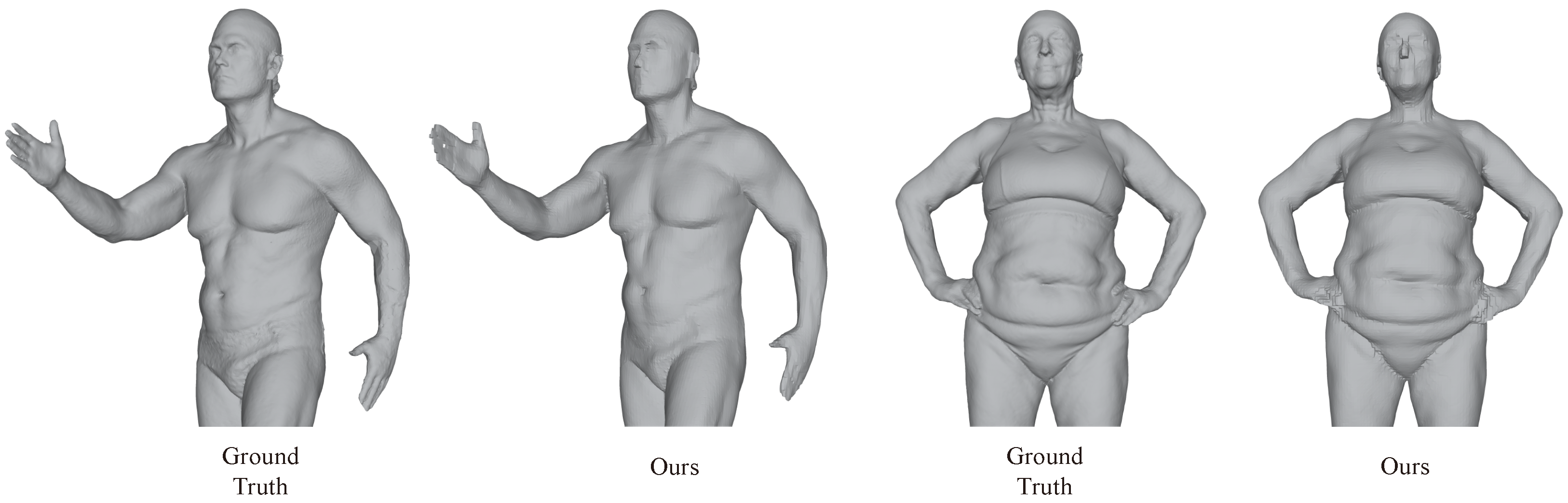
• The FAUST [44] dataset, which contains 100 human body models.
• The MGN dataset, a dataset containing clothes and open surfaces provided by MGN [45].
• Several rooms in the Matterport3D [46] dataset, which is used to test large indoor scan scenes.
• Some real-scanned urban building data that we colllected ourselves.

4.2. Metircs

We quantitatively evaluate surface reconstructions by taking a uniform sample of 100,000 points from both the ground truth and predicted meshes and calculated the following metrics, which were used to evaluate surface reconstruction accuracy, sharp feature preservation, and algorithm efficiency.

Reconstruction accuracy. We used commonly used metrics such as Chamfer distance (CD) and F-Score (F1) to evaluate the overall mesh reconstruction accuracy. These metrics are commonly used to measure the fit of the surface and can reflect significant reconstruction errors. However, they may not be able to measure the visual effect and details, such as sharp features that have a significant impact on the visual effect. Therefore, we followed NDC’s approach and added the following two metrics to measure the reconstruction effect of sharp features and boundary details.

Sharp feature preservation. To measure the quality of boundary reconstruction, we used Edge Chamfer Distance (ECD) and Edge F-score (EF1). We replaced the uniform sampling with dense sampling near the boundary on both the ground truth and predicted shapes to calculate the above two metrics.

Algorithm efficiency. For learning-based methods, we used training time (per epoch/total time), training memory usage, and inference time to evaluate the efficiency of the algorithm. These metrics can reflect the training cost of users when using these methods and thus reflect the usability of the algorithm. For non-learning based methods such as Poisson reconstruction, we only evaluated their inference time. All timings were tested on a desktop computer equipped with one NVIDIA A100 80G GPU and a 16-core Intel i7 @2.8GHz CPU.

4.3. Comparison with Baseline

We first demonstrate the comparison results with the baseline to verify the efficiency and improvement of HRE-NDC for sharp edge details. Figure 8 and

Table 2. Quantitative results on the ABC test set, 16,384 points as input.

Method	CD $\downarrow \left({10}^5\right)$	F1↑	EDC$\downarrow \left({10}^2\right)$	EF1↑	Inference Time
UNDC (baseline)	0.827	0.873	0.411	0.757	$1.281$ s
HRE-NDC (ours)	0.747	0.768	0.379	0.856	$2.934$ s

show the reconstruction results of three scales (${256}^3+{128}^3+{64}^3$) of HRE-NDC and UNDC (${256}^3$) with the same resolution; the objects shown in Figure 8 are all from the test set of the ABC dataset. It can be seen that although UNDC has produced decent reconstruction models, there are still issues with holes, artifacts and jagged edges on the boundary (as indicated in the red box in the figure; please zoom in to examine the specifics). Due to the coarse-to-fine structure of HRE-NDC and improvements targeting boundary details (residuals + activation), our method achieves better reconstruction quality, especially in sharp edge reconstruction. More importantly, our method significantly shortens training time.

Table 1 records the training strategies and durations of the results in Figure 8. It can be seen that HRE-NDC greatly reduces training time and GPU memory usage compared to the baseline. Taking the ${256}^3$ resolution training as an example, for fair comparison, the batch size of all methods in the table is set to 1 and trained and tested on the same NVIDIA A100 80G GPU. HRE-NDC in Figure 8 is trained according to the recommended strategy in Table 1, which is 60 epochs for ${64}^3$ resolution, 30 epochs for ${128}^3$ resolution, and 10 epochs for ${256}^3$ resolution, with a total training time of about $2.4$ days. However, according to the recommended strategy of UNDC, training 250 epochs takes about 26 days. Even if it is reduced to 100 epochs, as with our method, it still takes about $10.4$ days. Therefore, our method shortens the training time by 5–10× compared to the baseline.

Furthermore, our network uses sparse 3D-CNN instead of the “3DCNN + Mask” approach of NDC. HRE-NDC occupies 41 G of GPU memory when training at the highest resolution, and more than half of the remaining time, the GPU memory usage is no more than 12 G. This is a significant reduction compared to the baseline, which requires more than 70 G of GPU memory throughout the training process. Moreover, this allows for the use of larger batch sizes at lower resolution, further reducing the overall training time.

4.4. Comparison with Other NIR-Based Methods

We conducted a comparison between our method and other state-of-the-art Neural Implicit Representation (NIR)-based techniques, as presented in Figure 9 and

Table 3. Quantitative results on the Thingi10k dataset, 16,384 points as input.

Method	CD $\downarrow \left({10}^5\right)$	F1 ↑	EDC ↓	EF1 $\uparrow \left({10}^2\right)$	Inference Time
Points2Surf	7.954	0.428	8.686	0.042	$32.647$ s
LIG	4.642	0.768	11.652	0.025	$66.835$ s
ConvONet-3p	18.134	0.536	4.113	0.105	$2.692$ s
ConvONet-grid32	8.844	0.488	9.701	0.036	$2.404$ s
UNDC	0.753	0.873	0.822	0.757	$1.694$ s
HRE-NDC(ours)	0.726	0.832	0.752	0.856	$2.505$ s

. To ensure a fair assessment of their generalization performance, we trained these methods on their respective datasets according to the recommended settings of their authors and tested them on a new dataset, Thingi10k [43]. Our model was trained on the ABC train set according to the strategy recommended in Table 1.

For more details about these methods, please refer to Section 2.1. Figure 9 illustrates that these learning-based approaches have more or less limitations in generalization performance when making predictions on new datasets, and their performance is inferior to that of their original training datasets.

Specifically, Points2Surf [7] utilizes both “global” and “local” latent vectors to learn the occupancy of each point based on query points. However, its surface may have artifacts or jagged textures, as indicated by the red boxes, and the “occupancy + global latent vector” approach may not be conducive to learning and representing open surfaces or hollow holes, as shown by the blue box.

LIG [8] represents “parts” with latent vectors instead of the entire object, resulting in a more “local” approach with better generalization performance. However, since it relies on Marching Cubes [14,15] to reconstruct the mesh, it cannot produce sharper boundaries. Moreover, it may have “back-face” issues, as mentioned in their paper. Although they proposed a post-processing method to mitigate this problem, it still exists in some shapes, as shown by the yellow boxes.

Convolutional Occupancy Networks (ConvONet) [9] proposes two networks that use 2D-CNN and 3D-CNN, respectively named ConvONet-3plane (shown as ConvONet-3p in the Figure 9) and ConvONet-grid (shown as ConvONet-grid32 in the Figure 9, with a default resolution of ${32}^3$). We compared the performance of both models. The 3-plane network is more efficient but has inferior representation capabilities, which may lead to artifacts in the reconstruction results, as depicted by the red boxes. The grid model has better representation capabilities but is relatively less efficient. Additionally, since ConvONet uses one latent vector to represent one object, it may make semantic recognition errors and may not be as local as Points2surf or LIG, as shown by the green boxes. Finally, it also struggles to represent open surfaces and hollow holes well, as indicated by the blue boxes.

In comparison, our method achieves the best reconstruction results, with outstanding generalization performance and the ability to preserve clear and sharp boundaries.

4.5. Reconstruction of Large Scenes

Figure 10 and Figure 11 show the reconstruction results of our method applied to point clouds of large-scale indoor and urban building scenes. The point cloud of the indoor scene was sourced from the Matterport3D [46] dataset, while the point cloud of the urban building scene was collected by ourselves. Both are real scanned point clouds. Our network was trained only on the ABC [42] dataset without any specific training on similar scanned data, indicating its remarkable generalization and transferability.

Specifically, as shown in Figure 10, we compared our method with the commonly used traditional reconstruction method Screened Poisson (SCP) [25] and the recent outstanding learning-based method ConvONet [9]. From the enlarged detail map, we observe the following: (1) SCP relies on the input normals to differentiate between inside and outside in the local area, rather than an “unsigned” representation, which can lead to deformation. ConvONet may reconstruct better in one direction due to the utilization of an assumed reference plane, while other directions may yield inferior results. This can be seen in the bottom left of Figure 10, where the effect on the vertical ground direction is fine, while the effect on the wall is worse. Our method uses an “unsigned” representation and achieves relatively the best scene reconstruction effect. (2) SCP and ConvONet both employ Marching Cubes [14,15] to generate meshes, which can result in insufficiently sharp boundary representation. Our method employs Dual Contouring [24] to produce meshes, thus yielding higher-quality boundaries in the generated results.

4.6. Generalization Performance Demonstration

As mentioned in Section 2.1, in NIR-based reconstruction tasks, a “local” design means better generalization performance. To further demonstrate the generalization performance of our method, we present the reconstruction results on the clothing data provided by MGN [45] and the human body dataset FAUST [44]. Same as before, we only trained our network on the ABC dataset.

Figure 12 shows the reconstruction results on the clothing data, where higher resolution leads to more natural and realistic results in fabric texture. Interestingly, the input point clouds are randomly sampled from the ground truth meshes, and after our coarse-to-fine reconstruction, we achieve better surface details and transitions than the ground truth. Moreover, compared to the fixed-resolution UNDC, our mesh surface also looks more natural visually.

However, reconstructing human body shapes is relatively more challenging, as shown in Figure 13. Although our method accurately restores the human body, there are some distortions in details such as the face and fingers, which can be improved in future work.

5. Conclusions

This paper presents a summary and analysis of recent representative works in the field of Neural Implicit Representation-based reconstruction, highlighting several important insights. However, a major challenge with existing methods is their inability to handle high-resolution meshes efficiently. To address this issue, we propose HRE-NDC, which combines the strengths of previous methods and utilizes a coarse-to-fine network structure design with feature-preserving downsampling, residual prediction, and improved activation functions. HRE-NDC significantly reduces training time and memory usage while achieving better surface reconstruction results. Through a series of experiments, we demonstrate the superiority of HRE-NDC in both visualization and quantitative results and showcase its excellent generalization performance on diverse datasets, including large indoor scenes, urban buildings, clothing, and human body data.

Future work. NIR-based surface mesh reconstruction has shown remarkable performance with the advanced “feature grid + 3D-CNN” strategy, which possesses strong neighborhood information aggregation ability and is suitable for mesh reconstruction tasks. With the recent impressive performance of transformers [47,48,49] on visual and multimodal tasks, we are interested in exploring whether transformers combined with point convolution, with reasonable inductive bias, can perform well in reconstruction tasks. This will be a direction for our future work.

References

1. Berger, M.; Tagliasacchi, A.; Seversky, L.M.; Alliez, P.; Levine, J.a.; Sharf, A.; Silva, C.T.; Tagliasacchi, A.; Seversky, L.M.; Silva, C.T.; et al. State of the Art in Surface Reconstruction from Point Clouds. In Proceedings of the Eurographics 2014–State of the Art Reports, Strasbourg, France, 7 April 2014; Volume 1, pp. 161–185. [Google Scholar]
2. Berger, M.; Tagliasacchi, A.; Seversky, L.M.; Alliez, P.; Guennebaud, G.; Levine, J.A.; Sharf, A.; Silva, C.T. A Survey of Surface Reconstruction from Point Clouds. Comput. Graph. Forum 2017, 36, 301–329. [Google Scholar] [CrossRef]
3. Kaiser, A.; Ybanez Zepeda, J.A.; Boubekeur, T. A Survey of Simple Geometric Primitives Detection Methods for Captured 3D Data. Comput. Graph. Forum 2019, 38, 167–196. [Google Scholar] [CrossRef]
4. Chen, Z.; Zhang, H. Learning Implicit Fields for Generative Shape Modeling. In Proceedings of the IEEE Conference on Computer Vision and Pattern Recognition (CVPR), Long Beach, CA, USA, 15–20 June 2019. [Google Scholar]
5. Park, J.J.; Florence, P.; Straub, J.; Newcombe, R.; Lovegrove, S. DeepSDF: Learning Continuous Signed Distance Functions for Shape Representation. In Proceedings of the IEEE Conference on Computer Vision and Pattern Recognition (CVPR), Long Beach, CA, USA, 15–20 June 2019. [Google Scholar]
6. Mescheder, L.; Oechsle, M.; Niemeyer, M.; Nowozin, S.; Geiger, A. Occupancy Networks: Learning 3D Reconstruction in Function Space. In Proceedings of the IEEE Conference on Computer Vision and Pattern Recognition (CVPR), Long Beach, CA, USA, 15–20 June 2019. [Google Scholar]
7. Erler, P.; Guerrero, P.; Ohrhallinger, S.; Mitra, N.J.; Wimmer, M. Points2Surf: Learning Implicit Surfaces from Point Clouds. In Computer Vision—ECCV 2020, Proceedings of the 16th European Conference, Glasgow, UK, 23–28 August 2020; Springer International Publishing: Cham, Switzerland, 2020; pp. 108–124. [Google Scholar] [CrossRef]
8. Jiang, C.M.; Sud, A.; Makadia, A.; Huang, J.; Nießner, M.; Funkhouser, T. Local Implicit Grid Representations for 3D Scenes. In Proceedings of the IEEE Conference on Computer Vision and Pattern Recognition (CVPR), Seattle, WA, USA, 13–19 June 2020. [Google Scholar]
9. Songyou, P.; Michael, N.; Lars, M.; Marc, P.; Andreas, G. Convolutional Occupancy Networks. In Proceedings of the European Conference on Computer Vision (ECCV), Glasgow, UK, 23–28 August 2020. [Google Scholar]
10. Chen, Z.; Tagliasacchi, A.; Funkhouser, T.; Zhang, H. Neural Dual Contouring. ACM Trans. Graph. 2022, 41, 1–13. [Google Scholar] [CrossRef]
11. Fan, H.; Su, H.; Guibas, L.J. A point set generation network for 3D Object Reconstruction from a single Image. In Proceedings of the IEEE Conference on Computer Vision and Pattern Recognition, Honolulu, HI, USA, 21–26 July 2017; pp. 605–613. [Google Scholar]
12. Maturana, D.; Scherer, S. VoxNet: A 3D Convolutional Neural Network for real-time object recognition. In Proceedings of the 2015 IEEE/RSJ International Conference on Intelligent Robots and Systems (IROS), Hamburg, Germany, 28 September–2 October 2015; pp. 922–928. [Google Scholar] [CrossRef]
13. Groueix, T.; Fisher, M.; Kim, V.G.; Russell, B.C.; Aubry, M. A papier-mâché approach to learning 3D surface generation. In Proceedings of the IEEE Conference on Computer Vision and Pattern Recognition, Salt Lake City, UT, USA, 18–23 June 2018; pp. 216–224. [Google Scholar]
14. Lorensen, W.E.; Cline, H.E. Marching Cubes: A High Resolution 3D Surface Construction Algorithm. ACM SIGGRAPH Comput. Graph. 1987, 21, 163–169. [Google Scholar] [CrossRef]
15. Evgcni, V. Chernyacv Marching Cubes 33: Construction of Topologically Correct. 1995. Available online: https://cds.cern.ch/record/292771/files/cn-95-017.pdf (accessed on 14 January 2023).
16. Chibane, J.; Alldieck, T.; Pons-Moll, G. Implicit Functions in Feature Space for 3D Shape Reconstruction and Completion. In Proceedings of the IEEE Conference on Computer Vision and Pattern Recognition (CVPR), Seattle, WA, USA, 13–19 June 2020. [Google Scholar]
17. Krizhevsky, A.; Sutskever, I.; Hinton, G.E. ImageNet Classification with Deep Convolutional Neural Networks. Commun. ACM 2017, 60, 84–90. [Google Scholar] [CrossRef]
18. Simonyan, K.; Zisserman, A. Very deep convolutional networks for large-scale image recognition. arXiv 2014, arXiv:1409.1556. [Google Scholar]
19. He, K.; Zhang, X.; Ren, S.; Sun, J. Deep residual learning for image recognition. In Proceedings of the IEEE Conference on Computer Vision and Pattern Recognition, Las Vegas, NV, USA, 27–30 June 2016; pp. 770–778. [Google Scholar]
20. Huang, G.; Liu, Z.; Van Der Maaten, L.; Weinberger, K.Q. Densely connected convolutional networks. In Proceedings of the IEEE Conference on Computer Vision and Pattern Recognition, Honolulu, HI, USA, 21–26 July 2017; pp. 4700–4708. [Google Scholar]
21. Chen, Z.; Zhang, H. Neural Marching Cubes. ACM Trans. Graph. 2021, 40, 1–15. [Google Scholar] [CrossRef]
22. Rumelhart, D.; Hinton, G.; Williams, R. Learning representations by back-propagating errors. Nature 1986, 323, 533–536. [Google Scholar] [CrossRef]
23. Hinton, G. Fast Learning of Sparse Representations with an Energy-Based Model. Neural Comput. 2006, 18, 1527–1554. [Google Scholar] [CrossRef]
24. Ju, T.; Losasso, F.; Schaefer, S.; Warren, J. Dual Contouring of Hermite Data. ACM Trans. Graph. 2002, 21, 339–346. [Google Scholar] [CrossRef]
25. Kazhdan, M.; Hoppe, H. Screened poisson surface reconstruction. ACM Trans. Graph. 2013, 32, 1–13. [Google Scholar] [CrossRef]
26. Hinton, G.E.; Salakhutdinov, R.R. Reducing the dimensionality of data with neural networks. Science 2006, 313, 504–507. [Google Scholar] [CrossRef]
27. Kingma, D.; Welling, M. Auto-Encoding Variational Bayes. arXiv 2013, arXiv:1312.6114. [Google Scholar]
28. Chang, A.X.; Funkhouser, T.; Guibas, L.; Hanrahan, P.; Huang, Q.; Li, Z.; Savarese, S.; Savva, M.; Song, S.; Su, H.; et al. Shapenet: An information-rich 3d model repository. arXiv 2015, arXiv:1512.03012. [Google Scholar]
29. Choy, C.B.; Xu, D.; Gwak, J.; Chen, K.; Savarese, S. 3D-R2N2: A Unified Approach for Single and Multi-view 3D Object Reconstruction. In Proceedings of the European Conference on Computer Vision (ECCV), Amsterdam, The Netherlands, 11–14 October 2016. [Google Scholar]
30. Garland, M.; Heckbert, P.S. Surface Simplification Using Quadric Error Metrics. In Proceedings of the 24th Annual Conference on Computer Graphics and Interactive Techniques, New York, NY, USA, 3 August 1997; ACM Press: New York, NY, USA; Addison-Wesley Publishing Co.: Boston, MA, USA, 1997; pp. 209–216. [Google Scholar] [CrossRef]
31. Chibane, J.; Mir, A.; Pons-Moll, G. Neural Unsigned Distance Fields for Implicit Function Learning. In Proceedings of the Advances in Neural Information Processing Systems (NeurIPS), Vancouver, BC, Canada, 6–12 December 2020. [Google Scholar]
32. Qi, C.R.; Su, H.; Mo, K.; Guibas, L.J. Pointnet: Deep learning on point sets for 3D classification and segmentation. In Proceedings of the IEEE Conference on Computer Vision and Pattern Recognition, Honolulu, HI, USA, 21–26 July 2017; pp. 652–660. [Google Scholar]
33. Qi, C.R.; Yi, L.; Su, H.; Guibas, L.J. PointNet++: Deep Hierarchical Feature Learning on Point Sets in a Metric Space. In Proceedings of the 31st International Conference on Neural Information Processing Systems, Long Beach, CA, USA, 4 December 2017; Curran Associates Inc.: Red Hook, NY, USA, 2017; pp. 5105–5114. [Google Scholar]
34. Alliez, P.; Giraudot, S.; Jamin, C.; Lafarge, F.; Mérigot, Q.; Meyron, J.; Saboret, L.; Salman, N.; Wu, S.; Yildiran, N.F. Point Set Processing. In CGAL User and Reference Manual, 5.1th ed.; 2022; Available online: https://geometrica.saclay.inria.fr/team/Marc.Glisse/tmp/cgal-power/Manual/how_to_cite_cgal.html (accessed on 20 March 2023).
35. Rusu, R.B.; Cousins, S. 3D is here: Point Cloud Library (PCL). In Proceedings of the IEEE International Conference on Robotics and Automation (ICRA), Shanghai, China, 9–13 May 2011; IEEE: Piscataway, NJ, USA, 2011. [Google Scholar]
36. Dumoulin, V.; Visin, F. A guide to convolution arithmetic for deep learning. arXiv 2016, arXiv:1603.07285. [Google Scholar]
37. Paszke, A.; Gross, S.; Massa, F.; Lerer, A.; Bradbury, J.; Chanan, G.; Killeen, T.; Lin, Z.; Gimelshein, N.; Antiga, L.; et al. Pytorch: An imperative style, high-performance deep learning library. Adv. Neural Inf. Process. Syst. 2019, 32, 8024–8035. [Google Scholar]
38. Abadi, M.; Agarwal, A.; Barham, P.; Brevdo, E.; Chen, Z.; Citro, C.; Corrado, G.S.; Davis, A.; Dean, J.; Devin, M.; et al. Tensorflow: Large-scale machine learning on heterogeneous distributed systems. arXiv 2016, arXiv:1603.04467. [Google Scholar]
39. Redmon, J.; Divvala, S.; Girshick, R.; Farhadi, A. You Only Look Once: Unified, Real-Time Object Detection. In Proceedings of the IEEE Conference on Computer Vision and Pattern Recognition (CVPR), Las Vegas, NV, USA, 27–30 June 2016. [Google Scholar]
40. Graham, B.; Engelcke, M.; van der Maaten, L. 3D Semantic Segmentation with Submanifold Sparse Convolutional Networks. In Proceedings of the IEEE Conference on Computer Vision and Pattern Recognition (CVPR), Salt Lake City, UT, USA, 18–23 June 2018. [Google Scholar]
41. Graham, B.; van der Maaten, L. Submanifold Sparse Convolutional Networks. arXiv 2017, arXiv:1706.01307. [Google Scholar]
42. Koch, S.; Matveev, A.; Williams, F.; Alexa, M.; Zorin, D.; Panozzo, D.; Files, C.A.D. ABC: A Big CAD Model Dataset For Geometric Deep Learning. arXiv 2018, arXiv:1812.06216. [Google Scholar]
43. Zhou, Q.; Jacobson, A. Thingi10K: A Dataset of 10,000 3D-Printing Models. arXiv 2016, arXiv:1605.04797. [Google Scholar]
44. Bogo, F.; Romero, J.; Loper, M.; Black, M.J. FAUST: Dataset and Evaluation for 3D Mesh Registration. In Proceedings of the 2014 IEEE Conference on Computer Vision and Pattern Recognition, Columbus, OH, USA, 23–28 June 2014; pp. 3794–3801. [Google Scholar] [CrossRef]
45. Bhatnagar, B.; Tiwari, G.; Theobalt, C.; Pons-Moll, G. Multi-Garment Net: Learning to Dress 3D People From Images. In Proceedings of the 2019 IEEE/CVF International Conference on Computer Vision (ICCV), Seoul, Korea, 27 October 2019; pp. 5419–5429. [Google Scholar] [CrossRef]
46. Chang, A.; Dai, A.; Funkhouser, T.; Halber, M.; Niessner, M.; Savva, M.; Song, S.; Zeng, A.; Zhang, Y. Matterport3D: Learning from RGB-D Data in Indoor Environments. In Proceedings of the 7th IEEE International Conference on 3D Vision, 3DV 2017, Qingdao, China, 10–12 October 2017. [Google Scholar]
47. Vaswani, A.; Shazeer, N.; Parmar, N.; Uszkoreit, J.; Jones, L.; Gomez, A.N.; Kaiser, Ł.; Polosukhin, I. Attention is all you need. Adv. Neural Inf. Process. Syst. 2017, 30, 6000–6010. [Google Scholar]
48. Dosovitskiy, A.; Beyer, L.; Kolesnikov, A.; Weissenborn, D.; Zhai, X.; Unterthiner, T.; Dehghani, M.; Minderer, M.; Heigold, G.; Gelly, S.; et al. An image is worth 16x16 words: Transformers for image recognition at scale. arXiv 2020, arXiv:2010.11929. [Google Scholar]
49. Radford, A.; Kim, J.W.; Hallacy, C.; Ramesh, A.; Goh, G.; Agarwal, S.; Sastry, G.; Askell, A.; Mishkin, P.; Clark, J.; et al. Learning transferable visual models from natural language supervision. In Proceedings of the International Conference on Machine Learning, PMLR, Virtual, 18–24 July 2021; pp. 8748–8763. [Google Scholar]
Figure 1. Comparison with previous state-of-the-art method. UNDC [10] may encounter representation blurring when operating at low resolutions (top-right: UNDC at 64 3 ). Simply increasing the resolution can result in unbearable complexity and training time(Table 1), while boundary defects may still persist (bottom-left: UNDC at 256 3 ). Our method not only significantly reduces training time (Table 1) but also achieves better boundary quality (bottom-right: HRE-NDC at 256 3 + 128 3 + 64 3 ).
Remotesensing 15 02267 g001
Figure 2. Marching Cubes (MC) [14] and Dual Contouring (DC) [24]. The blue dots represent intersection points in MC and vertices in DC.
Remotesensing 15 02267 g002
Figure 3. The network architecture of NDC and UNDC.
Remotesensing 15 02267 g003
Figure 4. Unsigned NDC. The “+” and “−” represent the occupancy of each edge, and the blue dots represent vertices within each cell.
Remotesensing 15 02267 g004
Figure 5. The network architecture of HRE-NDC.
Remotesensing 15 02267 g005
Figure 6. Feature-preserving downsampling. The “+” and “−” represent the occupancy of each edge.
Remotesensing 15 02267 g006
Figure 7. Upsampling without interpolation. The “+” and “−” represent the occupancy of each edge, and the colored dots correspond to the same-colored grid cells and represent the upsampled vertices.
Remotesensing 15 02267 g007
Figure 8. Comparison with baseline. Results of reconstructing 3D mesh models from point cloud inputs of 16,384 points. The shapes are all from the ABC test set. Please zoom in to examine the specific details highlighted in the red box.
Remotesensing 15 02267 g008
Figure 9. Comparison with previous NIR-based methods. Results of reconstructing 3D mesh models from point cloud inputs. All the shapes are from the Thingi10k dataset, which is new for all these methods to evaluate their generalization performance. The red boxes indicate “artifacts or distortions”, the blue boxes indicate “inability to represent hollow objects”, the green box indicates “semantic errors”, and the yellow box indicates “back-face” (only occurs in LIG).
Remotesensing 15 02267 g009
Figure 10. Reconstruction of the large-scale indoor scene point cloud, which is real-scanned data from the Matterport3D dataset.
Remotesensing 15 02267 g010
Figure 11. Reconstruction results on a real-scanned urban building point cloud. Compared to conventional reconstruction methods such as Screened Poisson [25], our approach can more accurately capture details and sharp edge features; it exhibits excellent generalization performance and also eliminates the need for separate training for different data.
Remotesensing 15 02267 g011
Figure 12. Mesh reconstruction results from point cloud inputs on two cloth shapes from the MGN dataset.
Remotesensing 15 02267 g012
Figure 13. Mesh reconstruction results from point cloud inputs on two human body shapes from the FAUST dataset.
Remotesensing 15 02267 g013