Enhancing the Accuracy of Boresight Calibration with Coplanarity Constraint and Relative Height from DEM

Abstract

As the resolution of airborne hyperspectral imagers (AHIs) continues to improve, the demand for accurate boresight calibration also increases. However, the high cost of ground control points (GCPs) and the low horizontal resolution of open digital elevation model (DEM) datasets limit the accuracy of AHI’s boresight calibration. We propose a method to enhance the accuracy of DEM-based boresight calibration using coplanarity constraints to address this issue. Our approach utilizes the relative accuracy of DEM in low-resolution DEM datasets. To make better use of the DEM, we apply coplanarity constraints to identify image features that display similar displacement in overlapping areas, and extract their corresponding elevation values from the DEM. These features and their relative heights are then incorporated into an optimization problem for boresight calibration. In the case of low-resolution DEM datasets, our method fully utilizes the relative accuracy of the DEM to improve the boresight correction precision. We have proven that the relative accuracy of elevation is more reliable than absolute accuracy in this situation. Our approach has been tested on the dataset from AHI, and the results have shown that the proposed method has better accuracy on low-resolution DEM datasets. In summary, our method provides a novel approach to improving the accuracy of DEM-based boresight calibration for AHIs, which can benefit applications, such as remote sensing and environmental monitoring. This research highlights the importance of utilizing the relative accuracy of low-resolution DEM datasets for improving the accuracy of boresight calibration.

1. Introduction

Hyperspectral imagery is a powerful tool that provides narrow bands data of observation targets, enabling the extraction of more detailed information about the physical and chemical properties of targets compared to multispectral imagery. The fine spectral imagery data cubes generated from hyperspectral imagery offer a platform for the quantitative analysis of the characteristics of observation targets [1]. With the advancements in computer hardware and efficient processing techniques, hyperspectral imagery has been widely used in various fields, such as precision agriculture [2,3,4], land resources management [5,6], water resource analysis [7,8], and natural disaster analysis [9].

In recent decades, hyperspectral imaging has been primarily conducted using spaceborne and airborne platforms. Spaceborne sensors offer more stable working conditions, fixed revisit periods, and higher efficiency. On the other hand, airborne sensors provide greater flexibility in observation planning, higher ground sample distance (GSD), and signal-to-noise ratio (SNR) [10]. Recently, unmanned aerial vehicles (UAVs) equipped with lightweight hyperspectral instruments have gained popularity due to their low operating costs and high flexibility [11]. UAV-borne instruments typically offer the highest GSD due to the low flight height of the UAVs. Consequently, they are well-suited for local observation tasks as compared to airborne sensors. In contrast, airborne advanced hyperspectral imagers (AHIs) have longer operation times and higher payloads, making them more advantageous for certain observation tasks.

Georeferencing is a fundamental step for hyperspectral imagery analysis. Two categories of georeferencing methods exist, direct and indirect georeferencing. Direct georeferencing utilizes Global Navigation Satellite System (GNSS) and Inertial Measurement Units (IMU) to acquire the position and orientation of each image frame [12]. In contrast, indirect georeferencing involves the extraction of image feature points, measurement of ground control points (GCPs), and bundle adjustment for position and orientation of each frame [13,14,15].

Accurate calibration of boresight is crucial to ensure the precision of direct georeferencing [16]. The imaging system’s high-precision GNSS and IMU sensors enable the projection of image data onto geographic coordinates without the need for costly ground control points (GCPs) [12]. However, errors in the extrinsic parameters between the imaging subsystem and IMU are inevitable during long-term usage and transformation of the hyperspectral imaging system, with the boresight error representing the rotational component of these errors. While displacement errors can be limited by mechanical constraints, boresight errors are difficult to constrain. The resulting extrinsic parameter errors at each moment of AHI operation introduces georeferencing mismatches, posing obstacles for successive applications [17].

Boresight calibration is easier to perform in a 2D focal plane array camera than in a push broom hyperspectral imager, which is because the former captures one 2D image per frame with a rigid projective relationship between all pixels [18]. The relationship between corresponding points from two images is described by epipolar geometry, which can be utilized with feature extraction methods, such as SIFT [19,20], SURF [21], or ORB [22], to find corresponding feature pairs. The boresight error between the camera and IMU can then be solved by the equation $AX=XB$ on Euclidean group [23]. This problem is referred to as hand–eye calibration in robotics [24]. In comparison, a pushbroom hyperspectral imager captures one 1D image per frame [25], and the 2D hyperspectral image is generated by georeferencing the 1D image with data from the IMU sensor. Therefore, epipolar geometry is not applicable.

To obtain correct orientation parameters in the imaging process, constraints such as the position of photographed points or epipolar geometry are necessary. Muller et al. [26] minimized the difference between GCPs and image points using collinearity equation linearized by a Taylor series and an iterative least squares fit. With the help of DEM data and 5 GCPs, the final mismatches are around 1 pixel. Lenz et al. [27] used the DEM and automatically extracted tie points to calibrate boresight in a mountainous area. They minimized the RMS error over the distance among corresponding tie points with Fletcher’s modified Levenberg–Marquard Algorithm [28], achieving final RMS residuals of 2∼4 pixels with the SURF [21] feature extraction method. Habib et al. [29] proposed three strategies for boresight calibration, achieving the lowest RMSE values with the third strategy, which improves the intersection of conjugate light rays corresponding to tie points. The third strategy demonstrated RMSE values of 2 pixels perpendicular to flight direction and about 1 pixel parallel to flight direction in six datasets.

Plane-based methods have been employed for Lidar boresight correction. Skaloud and Lichti [30] used least-squares adjustment with direct-georeferencing equations and common plane points to determine Lidar boresight angles and other parameters. Ref. [31] introduced a point-to-plane model to enhance accuracy. However, unlike Lidar data, depth information cannot be directly obtained from image data, making it challenging to correct camera boresight angles using plane constraints.

Traditional boresight calibration methods rely on costly GCPs and calibration flights, which are not suitable for large-area observation tasks. To address the limitations of traditional methods and improve calibration accuracy, we propose a novel boresight calibration method that utilizes open DEM datasets with the coplanarity constraint. The coplanarity constraint is achieved by extracting features with similar disparity to retrieving their relative height from the DEM based on the direct georeferencing location. This approach also reduces the influence of shadows and buildings on relative height retrieval. Finally, we use an optimization method to find the optimal solution among overlapping areas with the relative height derived from DEM. The Airborne Multi-Modality Imaging Spectrometer (AMMIS) is an advanced hyperspectral imaging system developed by the Shanghai Institute of Technical Physics, Chinese Academy of Sciences, with the purpose of facilitating the efficient and extensive acquisition of hyperspectral data cubes. We validated the proposed method on the dataset collected by the AMMIS hyperspectral imager and open DEM datasets. The results demonstrated that the proposed method significantly improves the calibration accuracy, particularly in cases of low-resolution DEM data, and exhibits better consistency across different open DEM datasets.

2. Materials

2.1. Introduction of Instrument

Table 1. Core parameters of AMMIS VNIR hyperspectral imaging subsystem.

Parameter	VNIR
Wavelength Range (nm)	400–1000
FOV (degrees)	40
IFOV (mrad)	0.25
Focal Length (mm)	128
Spectral Bands	256
Cross Track Pixels	2836
Pixel Size ($\mathsf{\mu }$m)	32
Data Resolution (bit)	16

presents the fundamentalparameters of the VNIR subsystem of AMMIS. AMMIS employsthe POS AV610 system from Applanix Corporation for positioning and orientation.

2.2. Introduction of Dataset

2.2.1. Airborne Hyperspectral Imagery

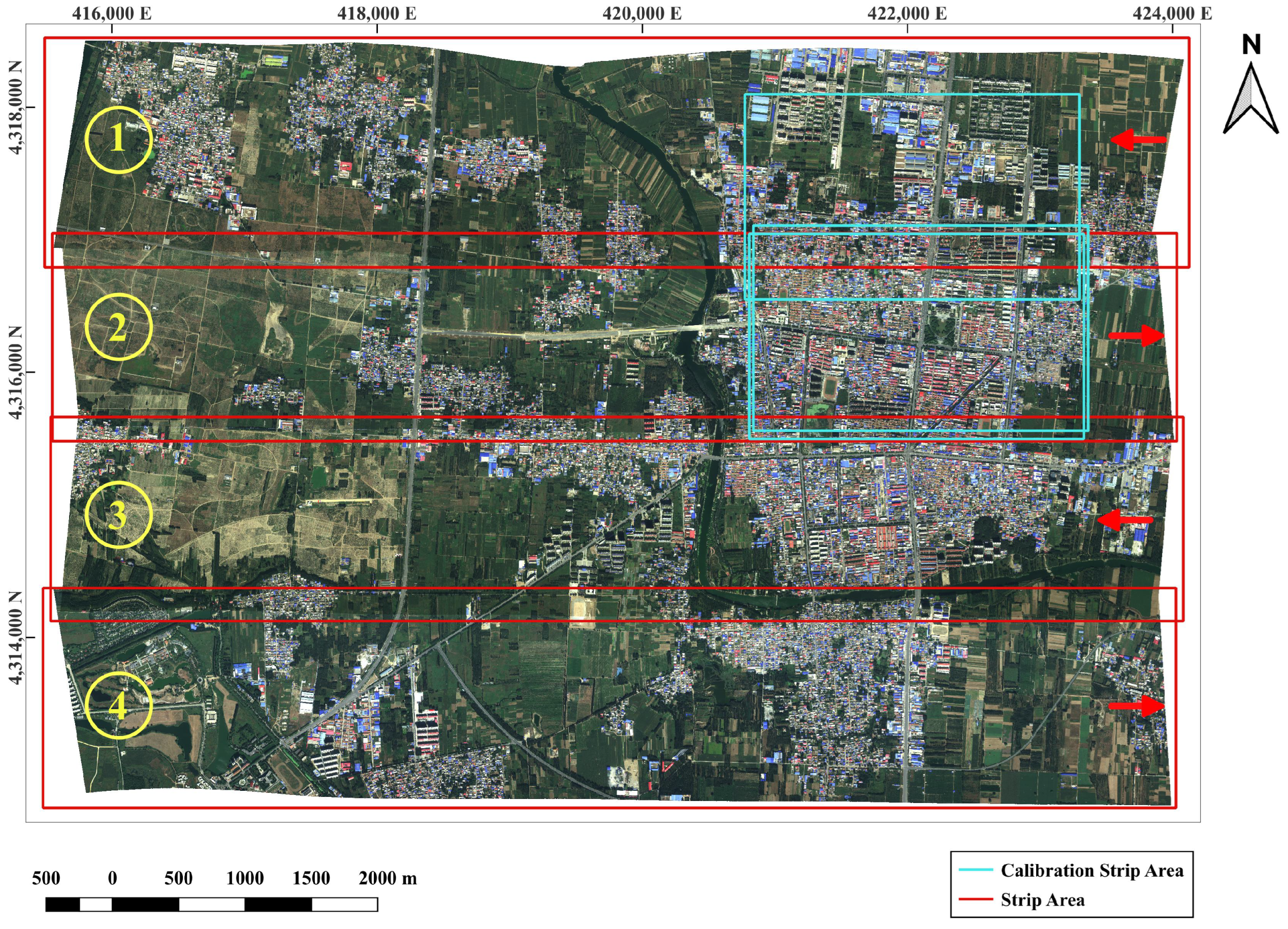
The calibration dataset was obtained by capturing images using the Airborne Multi-Modality Imaging Spectrometer (AMMIS) on the fixed wing aircraft Yun-5, at Xiongan, Hebei, China on 22 September 2018. The average flight height was 2100 m, and the ground sample distance (GSD) was 0.525 m. The average overlap ratio between adjacent strips was 15%. Given the large field of view (FOV), the observation task was accomplished over a vast area of 28 km × 48 km in two days, consisting of 20 strips. For validation purposes, we selected four strips, and more than 20,000 image lines were chosen from each strip. In the interest of efficiency, the raw dataset used was the RGB image, where the blue band wavelength was 473.6826 nm, the green band wavelength was 559.1906 nm, and the red band wavelength was 673.5705 nm. The four strips of the area are presented in Figure 1. Post-processing of POS data is performed using the IN-Fusion PPP mode of the POSPac MMS software, the RMS of pose data are shown in

Table 2. Maximum RMS of pose data after post-processing with IN-Fusion PPP mode.

Parameter	Roll (arc-min)	Pitch (arc-min)	Yaw (arc-min)	North (cm)	East (cm)	Down (cm)
Value	0.118	0.115	0.54	8.5	8	11.5

.

2.2.2. AW3D30

AW3D is a digital surface model (DSM) service, jointly developed and offered by the Remote Sensing Technology Center of Japan (RESTEC) and NTT DATA Corporation. It is photographed by the Panchromatic Remote Sensing Instrument for Stereo Mapping (PRISM) [32], which was an optical sensor on board the Advanced Land Observing Satellite (ALOS). More than 3 million satellite images are used to generate this dataset [33] by Multi-View Stereo Processing. AW3D is a commercial global digital surface model (DSM) with horizontal resolution of approximately 2.5 m/5 m [34]. AW3D30 is freely available with horizontal resolution 30 m. The data used for this paper have been provided by AW3D30 of the Japan Aerospace Exploration Agency.

2.2.3. ASTER GDEM V3

The Advanced Spaceborne Thermal Emission and Reflection Radiometer (ASTER) [35] Global Digital Elevation Model (GDEM) dataset is an open DEM datasets created by The Ministry of Economy, Trade, and Industry (METI) of Japan and the United States National Aeronautics and Space Administration (NASA). In June 2009, the first version of the ASTER GDEM was released. It was generated using stereo-pair images collected by the ASTER instrument onboard Terra. ASTER GDEM coverage spans from 83 degrees north latitude to 83 degrees south, encompassing 99% of Earth’s landmass. On 5 August 2019, NASA and METI published version 3 (V3) of ASTER GDEM. The improved GDEM V3 adds additional stereo-pairs, improving coverage and reducing the occurrence of artifacts.The ASTER GDEM V3 maintains the image format and the same gridding and tile structure as V1 and V2, with 30 m postings. The dataset is provided by Geospatial Data Cloud site, Computer Network Information Center, Chinese Academy of Sciences.

2.2.4. SRTM-GL1

The NASA Shuttle Radar Topography Mission (SRTM) dataset is the result of a joint effort between National Aeronautics and Space Administration (NASA) and the National Geospatial-Intelligence Agency, with participation from the German and Italian space agencies. The purpose of SRTM was to generate a near-global digital elevation model (DEM) of the Earth using radar interferometry. SRTM was a primary component of the payload on the Space Shuttle Endeavour during its STS-99 mission. Endeavour launched 11 February 2000 and flew for 11 days [36]. ALOS Phased Array L-band Synthetic Aperture Radar (PALSAR) was an active microwave sensor which was not affected by weather conditions and operable both day and night. It was based on a Synthetic Aperture Radar (SAR) carried onboard Japan’s first earth observation satellite [37]. ALOS PALSAR radiometrically terrain corrected (RTC) dataset was created by Alaska Satellite Facility to make SAR data accessible to a broader community of users [38]. In this paper, SRTM-GL1 datasets are the upsampling DEM version (horizontal resolution 12.5 m) from ALOS PAL RTC products.

The information of three open DEM datasets are shown in

Table 3. Summary of DEM datasets used in this paper.

Dataset	Horizontal Resolution (m)	RMSE (m)	Data Collection Period	Source
AW3D30	30	4.4 [39]	2006–2011	[40]
ASTER GDEM V3	30	8.52 [41]	2000–2013	[42]
SRTM-GL1	12.5	6.2 [43]	2000	[44]

.

3. Methods

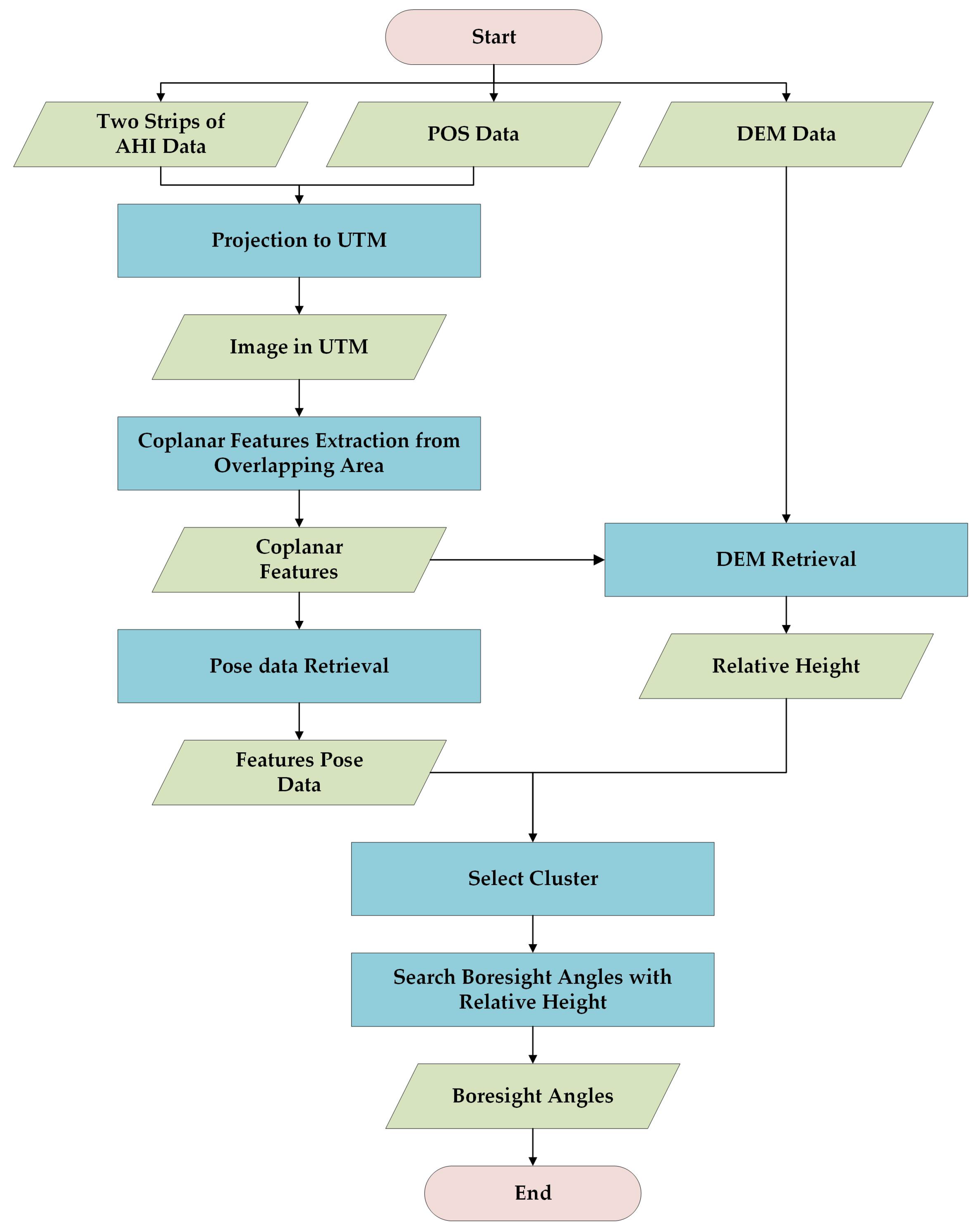
The pushbroom hyperspectral imaging system consists of two main subsystems, namely the imaging subsystem and the Inertial Measurement Unit (IMU) sensor. The IMU sensor plays a crucial role in recording pose and motion data of the system. However, it is unable to provide the relative pose with respect to the imaging subsystem, particularly the boresight angles. To address this limitation, we make an assumption that the boresight angles remain constant during an observation task. This section presents a detailed account of the proposed method, and a flow chart depicting the workflow is presented in Figure 2.

3.1. Projection to UTM

The projection of a hyperspectral image onto the Universal Transverse Mercator (UTM) coordinate system is a standard procedure. This procedure can be described as a process that converts pixel coordinates from the camera coordinate system to the Earth-Centered Earth-Fixed (ECEF) coordinate system. Subsequently, the pixel coordinates are converted from ECEF to the UTM coordinate system, and gridding is performed on the UTM grid. The conversion of pixel coordinates from the camera coordinate system to the ECEF coordinate system can be expressed by the following equation,

$$\begin{array}{cc}\hfill & {\mathbf{P}}_e={\mathbf{T}}_{NED}^{ECEF}{\mathbf{T}}_b^{NED}{\mathbf{T}}_c^b{\mathbf{P}}_c\hfill \\ \hfill & \mathbf{T}=\left[\begin{array}{cc}\mathbf{R}& \mathbf{t}\\ {\mathbf{0}}^{\top }& 1\end{array}\right]\hfill \end{array}$$

(1)

where ${\mathbf{P}}_e$ is the $4\times 1$ homogeneous location vector of a single pixel, ${\mathbf{P}}_c$ is the pixel coordinates in camera coordinate system, ${\mathbf{T}}_c^b$ is the transformation from the camera coordinate system to the IMU body coordinate system, ${\mathbf{T}}_b^{NED}$ is the transformation from the IMU body coordinate system to the North-East-Down (NED) coordinate system, ${\mathbf{T}}_{NED}^{ECEF}$ is the transformation from NED coordinate system to the ECEF coordinate system. The homogeneous vector can be expanded from its non-homogeneous vector, and the non-homogeneous location vector ${\mathbf{p}}_{\mathbf{c}}$ of ${\mathbf{P}}_c$ is derived from following equation

$${\mathbf{p}}_c=Z{\mathbf{K}}^{-1}{\mathbf{p}}_{uv}$$

(2)

where ${\mathbf{p}}_{uv}={(u,v,1)}^{\top }$ is the homogeneous coordinates of 2D image points, ${\mathbf{p}}_c={(X,Y,Z)}^{\top }$ is the non-homogeneous location of point in space corresponding to the pixel, $\mathbf{K}$ is the camera calibration matrix [18] of a camera, Z is the elevation measured by the GNSS/IMU sensor. Based on the coordinates in ECEF, we project the pixels to UTM coordinate system. Based on the pixel coordinates in ECEF, a projection is performed to transform the pixels onto the UTM coordinate system. Subsequently, an inverse distance to a power gridding technique [45] is applied to generate the gridding image.

3.2. Coplanar Features Extraction from Overlapping Area

Boresight calibration poses a challenge in determining the distance between the imaging system and the ground. Direct georeferencing allows us to obtain elevation data corresponding to the image data from the DEM data. However, utilizing the DEM elevation data for image features in boresight calibration has a drawback. The horizontal resolution of the open DEM is notably lower than the image data, resulting in the DEM elevation data corresponding to the image data being an averaged value. In the absence of elevation information, features at various elevations can affect the convergence values of the optimization problem. To address the aforementioned issues, this section proposes a coplanar feature extraction method to obtain features with similar elevation. By exploiting the characteristics of vertical imaging, two adjacent strip images can be treated as a stereo rig. Consequently, the displacement of the feature pair contains the depth information of the corresponding 3D point [46]. Since coplanar feature points have similar elevation data, we can utilize the DEM values of the coplanar feature points to estimate their average elevation data.

In addition to the variation in 3D point elevations, the difference between feature point pairs can also be influenced by the length of shadows over time. Therefore, feature points that satisfy the coplanarity constraint are less susceptible to the effect of shadows. The application of coplanarity constraint not only enhances the robustness of the feature points, but also improves the accuracy of subsequent processing.

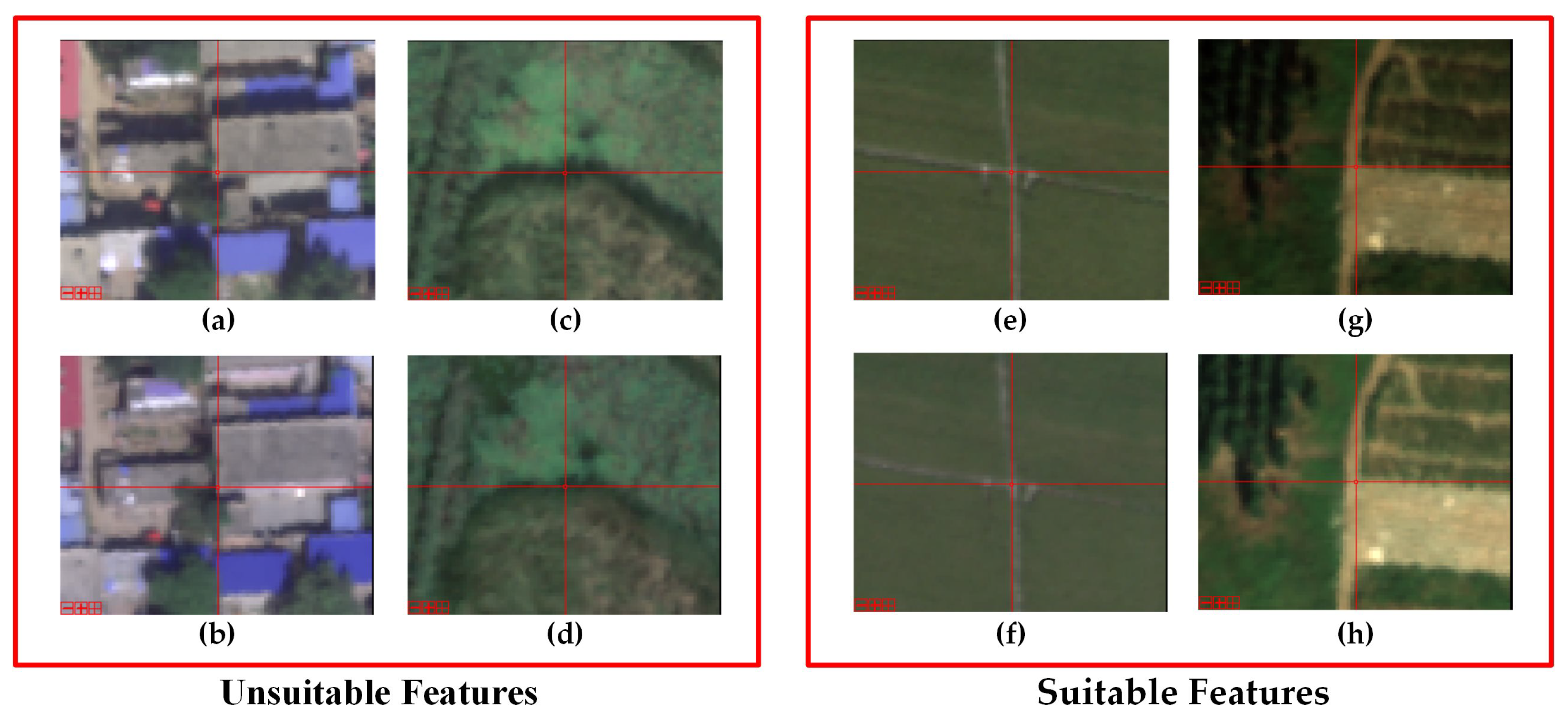
Feature extraction is conducted in pairs of adjacent strips. The procedure entails the use of the gridding image generated in Section 3.1. Subsequently, we applied the SIFT [19,20] feature extraction method and the RANSAC [47] feature filtering method to obtain the coarse features between the adjacent strips. These coarse features contain many unsuitable pairs that are related to shadow edges and elevation variations, as in the case of features located in building corners and shadow edges (as shown in Figure 3). After projection to UTM coordinates, the adjacent strip images can be viewed as a stereo rig, and the distance between the feature point pairs can be treated as disparity. While the distance between pairs of feature points is influenced by the error of boresight angles, this effect can be considered to be approximately consistent for these feature pairs. Assuming that we have a group of N coarse feature pairs, the Euclidean distance difference vector set G is represented as follows,

$$G=\{{\mathbf{g}}_i={\mathbf{p}}_i^f-{\mathbf{p}}_i^b,i=0,...,N-1\}$$

(3)

where ${\mathbf{p}}_i^f$ and ${\mathbf{p}}_i^b$ represent the coordinate vectors of a coarse feature pair in the UTM coordinate system. Based on the Euclidean distance difference vector set G obtained from the coarse feature pairs, clustering algorithms can be employed to identify suitable feature pairs. One such algorithm is the DBSCAN [48] algorithm, which can group feature points with similar disparities. The filtered feature points satisfying the coplanarity constraint are those with close elevation information, which indicates that they are located on the same elevation plane. Such feature points are referred to as fine-matching feature points and are more appropriate for subsequent processing.

3.3. Pose Data Retrieval

After filtering the coarse feature pairs, the remaining features require the retrieval of their pose data at the time of capture for subsequent processing, which is determined by the pushbroom imaging mode. In the rasterized image of a strip, each feature point along the flight direction is captured at almost different moments, and the moments corresponding to the feature points may lie between discrete image frames. It is assumed that each feature point is captured in a virtual frame between the actual image frames. Given that the pose data of each image frame are different, we use interpolation between image frames to retrieve the pose data of the virtual frame in which each feature is captured. The pose data of the virtual frame can be calculated using the following equation,

$$\begin{array}{cc}\hfill & \mathbf{a}={\mathbf{q}}_{w{b}_n}{\mathbf{a}}^{b_n}\hfill \\ \hfill & {\mathbf{q}}_w={\mathbf{q}}_{w{b}_n}\otimes \left[\begin{array}{c}\mathbf{1}\\ \frac{1}{2}{\omega }^{b_n}\delta t\end{array}\right]\hfill \\ \hfill & {\mathbf{v}}^w={\mathbf{v}}_n^w+\mathbf{a}\delta t\hfill \\ \hfill & {\mathbf{p}}^w={\mathbf{p}}_{b_n}^w+{\mathbf{v}}^w\delta t+\frac{1}{2}\mathbf{a}\delta t^2\hfill \end{array}$$

(4)

where ${\mathbf{p}}^w$, ${\mathbf{q}}_w$, $\mathbf{a}$, and ${\mathbf{v}}^w$ are the estimated position, orientation, acceleration, and velocity of the virtual frame of a photographed feature in the world coordinate system, respectively; ${\mathbf{p}}_{b_n}^w$ and ${\mathbf{v}}_n^w$ are the position and velocity in the world coordinate system at moment n which is the line nearest in space, closest, and early in time to the feature. ${\mathbf{q}}_{w{b}_n}$ is the quaternion from the IMU body coordinate system at moment n to the world coordinate system. ${\mathbf{a}}^{b_n}$ and ${\omega }^{b_n}$ are acceleration and angular velocity in the IMU body coordinate system of moment n. $\delta t$ is the estimated time deviating to the moment n, ⊗ represents the multiplication operation between two quaternions. To find the image frame n based on the projection of image frames in the UTM coordinate system with the UTM coordinates of the feature point, binary search is used. However, to improve computational efficiency, the exact $\delta t$ calculation is abandoned. Instead, the time between image frames $\left(n\right)$ and image frames $(n+1)$ is divided into M virtual frames to find the mth virtual frame ($m\in 0,...,M-1$) closest to the feature point.

3.4. DEM Retrieval

In this section, we employ DEM datasets to extract statistical information of the features that were extracted in Section 3.2. The UTM coordinates of the features are calculated using the direct georeferencing method described in Equation (2). However, since the true elevation data and boresight errors are unknown, we use the mid-points of the features in the UTM coordinate system as their location. Then, we retrieve the elevation data of the features from the DEM datasets based on their UTM coordinates. By analyzing the distribution of elevation of features in the overlapping area, we can obtain the average elevation data of this overlapping area.

3.5. Search Boresight Angles with Relative Height

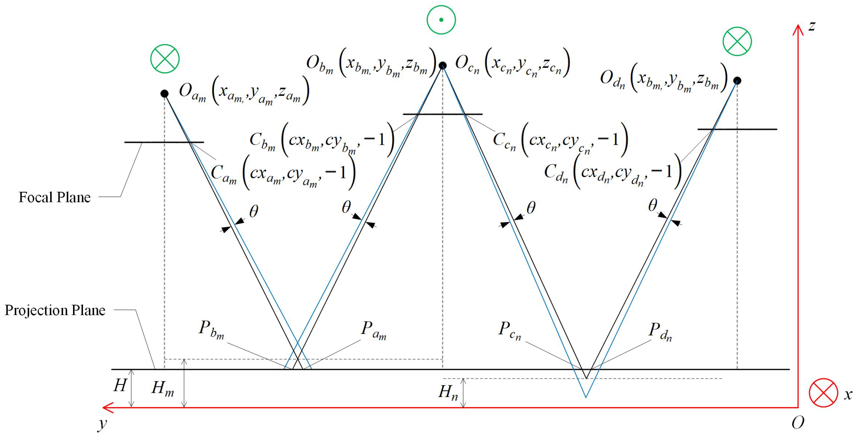
According to Habib et al. [29], the roll angle is a significant factor in determining the accuracy of the retrieved height. In our study, we focus on the effect of the roll angle error on the position of the projection point. To illustrate this effect, we use two pairs of feature points from adjacent strips as examples and present a 2D schematic figure to represent the 3D relationship of the adjacent overlapping areas, as shown in Figure 4. The coordinate system used in this study is the East-North-Up (ENU) coordinate system, which is similar to the UTM coordinate system in the local area. Based on this coordinate system, the projection error can be described as follows,   

$$\begin{array}{cc}\hfill & E(\theta ,H)=\sum _{m=0}^{M-1}{\mathbf{r}}_m^2+\sum _{n=0}^{N-1}{\mathbf{r}}_n^2\hfill \\ \hfill & =\sum _{m=0}^{M-1}{({\mathbf{P}}_{a_m}-{\mathbf{P}}_{b_m})}^{\top }({\mathbf{P}}_{a_m}-{\mathbf{P}}_{b_m})\hfill \\ \hfill & +\sum _{n=0}^{N-1}{({\mathbf{P}}_{c_n}-{\mathbf{P}}_{d_n})}^{\top }({\mathbf{P}}_{c_n}-{\mathbf{P}}_{d_n})\hfill \end{array}$$

(5)

where projection points $\{{\mathbf{P}}_{a_m},{\mathbf{P}}_{b_m},{\mathbf{P}}_{c_n},{\mathbf{P}}_{d_n}\}$ are expressed as below,

$$\begin{array}{cc}\hfill {\mathbf{P}}_{a_m}& =(H+z_{a_m})\mathrm{n}\left({\mathbf{R}}_{a_m}{\mathbf{R}}_{\varphi }{\mathbf{C}}_{a_m}\right)+{\mathbf{O}}_{a_m}\hfill \\ \hfill {\mathbf{P}}_{b_m}& =(H+z_{b_m})\mathrm{n}\left({\mathbf{R}}_{b_m}{\mathbf{R}}_{\varphi }{\mathbf{C}}_{b_m}\right)+{\mathbf{O}}_{b_m}\hfill \\ \hfill {\mathbf{P}}_{c_n}& =(H+z_{c_n})\mathrm{n}\left({\mathbf{R}}_{c_n}{\mathbf{R}}_{\varphi }{\mathbf{C}}_{c_n}\right)+{\mathbf{O}}_{c_n}\hfill \\ \hfill {\mathbf{P}}_{d_n}& =(H+z_{d_n})\mathrm{n}\left({\mathbf{R}}_{d_n}{\mathbf{R}}_{\varphi }{\mathbf{C}}_{d_n}\right)+{\mathbf{O}}_{d_n}\hfill \end{array}$$

(6)

where ${\mathbf{R}}_{\varphi }=exp\left({\varphi }^{\wedge }\right)$, $\varphi \in \mathfrak{se}\left(3\right)$ is boresight angles, $exp\left(\right)$ is the exponential map, ${\left(\right)}^{\wedge }$ converts a vector to its skew-symmetric matrix which satisfies ${\mathbf{a}}^{\wedge }=[0,-a_3,a_2;a_3,0,-a_1;-a_2,a_1,0]$, $\{{\mathbf{O}}_{a_m},{\mathbf{O}}_{b_m}\}$, and $\{{\mathbf{O}}_{c_n},{\mathbf{O}}_{d_n}\}$ are position vectors of optical centers in the ENU coordinate system, $\{{\mathbf{C}}_{a_m},{\mathbf{C}}_{b_m}\}$, and $\{{\mathbf{C}}_{c_n},{\mathbf{C}}_{d_n}\}$ are normalized intrinsic parameters of feature pairs, where $\mathrm{n}\left(\right)$ normalize the vector from ${(x,y,z)}^{\top }$ to ${(-x/z,-y/z,-1)}^{\top }$, ${\mathbf{R}}_{a_m},{\mathbf{R}}_{b_m}$ and ${\mathbf{R}}_{c_n},{\mathbf{R}}_{d_n}$ are nominal rotation matrix from the camera coordinate system to the ENU coordinate system, $z_{a_m}$, $z_{b_m}$, $z_{c_n}$ and $z_{d_n}$ are the elevation of imaging system. To simplify the presentation, the following definition is made,

$$\begin{array}{cc}\hfill \mathbf{t}& ={\mathbf{R}}_c^{ENU}{\mathbf{R}}_{\varphi }\mathbf{C}\hfill \\ \hfill \frac{\partial \mathrm{n}\left(\mathbf{t}\right)}{\partial \mathbf{t}}& =\left[\begin{array}{ccc}-\frac{1}{t_z}& 0& 0\\ 0& -\frac{1}{t_z}& 0\\ 0& 0& 0\end{array}\right]\hfill \\ \hfill \frac{\partial \mathbf{t}}{\partial \varphi }& =-{\mathbf{R}}_c^{ENU}{\left({\mathbf{R}}_{\varphi }\mathbf{C}\right)}^{\wedge }\hfill \end{array}$$

(7)

where ${\mathbf{R}}_c^{ENU}$ is the rotation matrix from the camera coordinate system to the ENU coordinate system, $\mathbf{C}$ is the intrinsic parameters for the corresponding feature point. We derived $\frac{\partial E}{\partial H}$ and $\frac{\partial E}{\partial \varphi }$ from the formula of $E(\varphi ,H)$, which are shown as follows:

$$\begin{array}{c}\hfill \frac{\partial {\mathbf{r}}_m}{\partial H}=\mathrm{n}\left({\mathbf{t}}_{a_m}\right)-\mathrm{n}\left({\mathbf{t}}_{b_m}\right)\\ \hfill \frac{\partial {\mathbf{r}}_n}{\partial H}=\mathrm{n}\left({\mathbf{t}}_{c_n}\right)-\mathrm{n}\left({\mathbf{t}}_{d_n}\right)\end{array}$$

(8)

and

$$\begin{array}{cc}\hfill \frac{\partial {\mathbf{r}}_m}{\partial \varphi }& =(H+z_{a_m})\frac{\partial \mathrm{n}\left({\mathbf{t}}_{a_m}\right)}{\partial {\mathbf{t}}_{a_m}}\frac{\partial {\mathbf{t}}_{a_m}}{\partial \varphi }-(H+z_{b_m})\frac{\partial \mathrm{n}\left({\mathbf{t}}_{b_m}\right)}{\partial {\mathbf{t}}_{b_m}}\frac{\partial {\mathbf{t}}_{b_m}}{\partial \varphi }\hfill \\ \hfill \frac{\partial {\mathbf{r}}_n}{\partial \varphi }& =(H+z_{c_n})\frac{\partial \mathrm{n}\left({\mathbf{t}}_{c_n}\right)}{\partial {\mathbf{t}}_{c_n}}\frac{\partial {\mathbf{t}}_{c_n}}{\partial \varphi }-(H+z_{d_n})\frac{\partial \mathrm{n}\left({\mathbf{t}}_{d_n}\right)}{\partial {\mathbf{t}}_{d_n}}\frac{\partial {\mathbf{t}}_{d_n}}{\partial \varphi }\hfill \end{array}$$

(9)

According to Figure 4, The yaw angles of ${\mathbf{R}}_{a_m}$ and ${\mathbf{R}}_{b_m}$, ${\mathbf{R}}_{c_n}$, and ${\mathbf{R}}_{d_n}$ differ by approximately ${180}^{\circ }$, the yaw angles of ${\mathbf{R}}_{b_m}$ and ${\mathbf{R}}_{c_n}$ are approximately equal, the values of ${\mathbf{C}}_{a_m}$ and ${\mathbf{C}}_{b_m}$, ${\mathbf{C}}_{c_n}$ and ${\mathbf{C}}_{d_n}$ are approximately equal. The roll and pitch angles are small because of gyro-stabilized sensor mount. Thus, combined with Equation (9), $\frac{\partial {\mathbf{r}}_m}{\partial \varphi }$ and $\frac{\partial {\mathbf{r}}_n}{\partial \varphi }$ have opposite signs. Additionally, $\frac{\partial E}{\partial \varphi }$ has a global minimum when $\varphi$ does not exceed a reasonable range. The blue lines in Figure 4 illustrate the variation of ${\mathbf{r}}_m$ and ${\mathbf{r}}_n$ about $\varphi$ and H.

If the extrinsic parameters of AHI and the elevation of feature points are correct, the projection error should be a zero vector. Take feature pairs from one of the overlapping area as an example. When ${\mathbf{r}}_m=\mathbf{0}$, the following equation can be derived,

$$\begin{array}{c}\hfill H_m(\mathrm{n}\left({\mathbf{t}}_{a_m}\right)-\mathrm{n}\left({\mathbf{t}}_{b_m}\right))=-z_{a_m}\mathrm{n}\left({\mathbf{t}}_{a_m}\right)+z_{b_m}\mathrm{n}\left({\mathbf{t}}_{b_m}\right)-({\mathbf{O}}_{a_m}-{\mathbf{O}}_{b_m})\end{array}$$

(10)

where $H_m$ is the true elevation value of the feature point. It is obvious that the $H_m$ and ${\mathbf{R}}_{\varphi }$ are corresponding. In addition, different strips share the same $\varphi$ because we assumed that the boresight angles do not change during the observation. Equation (10) implies a correspondence between the $\varphi$ and the respective mean height of each overlapping area.

According to the previous analysis, the minimum of ${\mathbf{r}}^2$ is determined once the extrinsic parameters and intrinsic parameters of features are fixed. The solution that satisfies the minimum is a good initialization of $\varphi$. The height information mainly influence the value of roll angle [29]. Thus, a three-step optimization is used for the final solution. We firstly use the Random Search (Algorithm 1) to find the ${\varphi }_0$ which makes ${\mathbf{r}}^2$ closest to zero according to the elevation data from POS. Secondly, we use the ${\varphi }_0$ as the initial value to search the $\varphi$ which makes height difference from triangulation of feature pairs equal to the value from DEM datasets. Only the roll angle is updated in this step. The loss function is defined as follows,

$$\begin{array}{c}\hfill L=\sum _i{(H_i\left(\varphi \right)-\overline{H}\left(\varphi \right)-(H_i^{DEM}-{\overline{H}}^{DEM}))}^2\end{array}$$

(11)

where $H_i\left(\varphi \right)$ is the elevation of ith overlapping area when given $\varphi$, $H_i^{DEM}$ is the elevation of ith overlapping area derived from DEM datasets. Finally, we apply the first step again to find the pitch and yaw angles with the roll angle fixed. When the overlapping area is more than two, the boresight calibration becomes an optimization problem. The procedure is present in the Algorithm 2.

Algorithm 1 Random Search method

Input: variables $\mathbf{x}$, data I, step $\lambda$, threshold $ϵ$, times T, loss function L; Output: variables ${\mathbf{x}}_f=(x_1,...,x_l)$    initialize $\mathbf{x}$, ${\mathbf{x}}_f$, $Los{s}_t=\infty$;    for $t=1\to T$do       random generate ${\mathbf{x}}_0$ = $(x_1,..x_l)(-1<x_i<1,i=1,...,l)$, $Loss=0$;       $\mathbf{x}$=$\mathbf{x}+\lambda *{\mathbf{x}}_0$;       for $m\in I$ do          $Loss=Loss+L(\mathbf{x},m)$;       end for       if $Loss<Los{s}_t$ then          $Los{s}_t=Loss$, ${\mathbf{x}}_f=\mathbf{x}$;       end if       if abs($Loss-Los{s}_t$)<$ϵ$ then          break;       end if end forreturn${\mathbf{x}}_f$;

Algorithm 2 Boresight calibration with Random Search

Input: Boresight angles $\varphi$, point pairs $I_m,m\in \{1,...,N\}$ from N overlapping area, DEM data $D_m,m\in \{1,...,N\}$, step for angle ${\lambda }_a$, step for projection plane ${\lambda }_h$, threshold $ϵ$, times T, loss function $L_1$(Equation (5)), $L_2$(Equation (11)); Output: Boresight angles $\varphi =({\varphi }_x,{\varphi }_y,{\varphi }_z)$   initialize $\varphi$;    optimize $\varphi$ and H by Algorithm 1 with $I_m$, ${\lambda }_a$, ${\lambda }_h$, $ϵ$, T and $L_1$;    optimize ${\varphi }_x$ by Algorithm 1 with $I_m$, $D_m$, ${\lambda }_a$, $ϵ$, T and $L_2$;    optimize ${\varphi }_y,{\varphi }_z$ by Algorithm 1 with $I_m$, ${\lambda }_a$, ${\lambda }_h$, $ϵ$, T and $L_1$;    return $\varphi$

4. Results and Analysis

4.1. Results of Feature Extraction

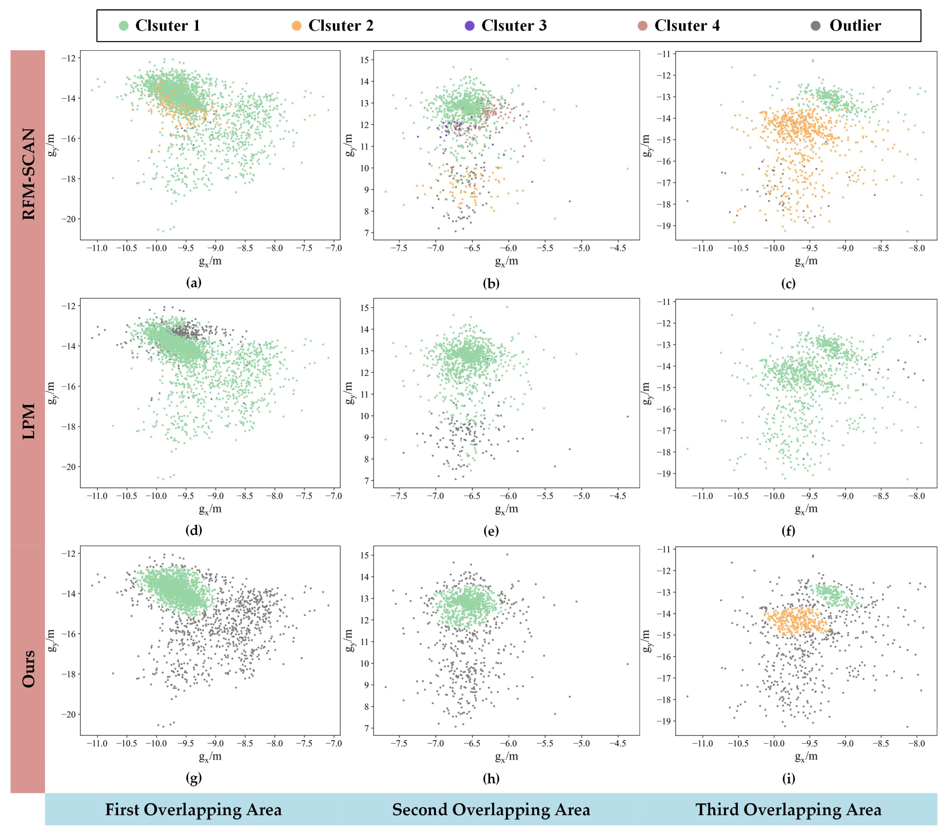
According to Equation (3), Figure 5 shows the distribution of Euclidean distance difference vector set G in different overlapping areas. As observed, there is at least one cluster in each overlapping area. The objective is to select these cluster points and determine their centers. Density-based spatial clustering of applications with noise (DBSCAN) [48] was utilized to select the clustering points, given that points in clusters are denser than those around the border. The parameters used were $maximum$ $distance=0.13$ and $minimum$ $samples=20$. The clustering results were then compared with other feature matching methods, such as LPM [49] (${\lambda }_1=0.9,{\lambda }_2=0.5,K=6,{\tau }_1=0.2,{\tau }_2=0.2$) and RFM-SCAN [50] ($\gamma =5,Bound=[5,45],Pct=0.2,\mu =[0,1,0.06]$). The proposed method could distinguish the clustering points from other feature points.

However, LPM assumes that the spatial relationship between the inliers is under a common transformation, making it unable to distinguish more than one cluster point in Figure 5f. In Figure 5d,e, LPM also includes features far away from the cluster. Additionally, RFM-SCAN supports the matching of more than one cluster, but the results include points far from the clusters. These methods are inadequate due to the large sizes of the images, the sparsely distributed feature points, as well as failure to take the effect of disparity between adjacent strips into consideration. To balance the feature numbers from different overlapping areas and improve processing speed, $K=120$ points of one cluster were selected from each overlapping area one time as a subset of suitable feature pairs. Feature points in the cluster were sampled uniformly to avoid changing the distribution of the clusters during later processing.

We established conventions for features in overlapping areas to simplify the representation. Specifically, we assigned index 1 to features from the overlapping area of the first and second strip, index 2 to features from the overlapping area of the second and third strip, and indexes 3 and 4 to cluster 1 and 2 features from the overlapping area of the third and fourth strip, as shown in Figure 5i.

4.2. Results of DEM Retrieval

This section presents partial results from the DEM retrieval analysis depicted in Figure 6 and Figure 7 for the third overlapping area. Cluster 1 (green marks) was found to correspond to low-lying areas in both the AW3D30 and SRTM-GL1 datasets, while the corresponding area in GDEM exhibited similar elevation to the surrounding areas, indicating lower accuracy compared to the other two DEMs. Cluster 2 (pink marks) corresponded to flat and open areas in all three DEM datasets. Moreover, the false color DEM image showed that the features located in open areas exhibited more uniform elevation data, which explained the improved accuracy achieved by using relative elevation estimates.

Our analysis also revealed that the horizontal resolution of the DEM significantly impacts retrieval accuracy. High-resolution features in images were significantly blurred in false color DEM image, resulting in averaged elevation estimates for feature points located in towns, as evidenced by the pink marks in Figure 6g. Furthermore, we observed varying data quality among different DEM datasets. Specifically, AW3D30 exhibited the sharpest edges and most consistent content with image data, as evidenced by the data from urban areas in Figure 6 and Figure 7, as well as data from river locations in Figure 7.

4.3. Results of Relative Height Determination with DEM

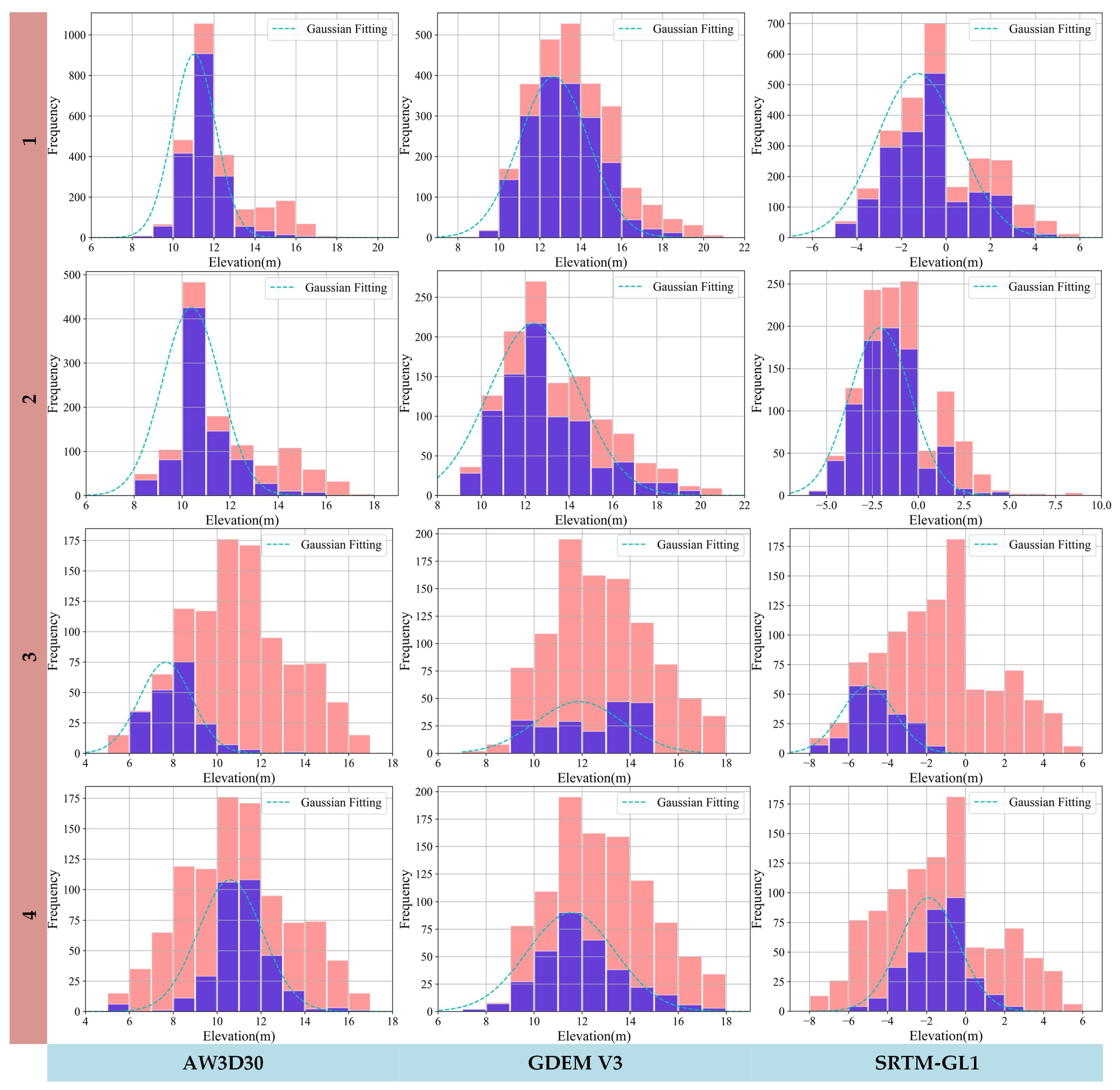
In this section, we present an elevation histogram of features located in the overlapping area. The elevation data were retrieved using three different DEM datasets, AW3D30, ASTER GDEM V3, and SRTM-GL1, while maintaining consistent UTM coordinates for each feature across all datasets.

Figure 8 reveals that the means of the retrieved elevation values differ among the DEM datasets. Additionally, the higher density of blue bins as compared to red bins suggests that the selected features possess similar elevation values.

Based on the data presented in

Table 4. Mean elevation and STD of elevation of selected features with different DEM datasets (m).

Overlapping Index	AW3D30	GDEM V3	SRTM-GL1
1	11.04 ± 1.05	12.7 ± 1.7	11.0 ± 1.86
2	10.38 ± 1.21	12.4 ± 2.06	10.17 ± 1.66
3	7.66 ± 1.2	11.88 ± 1.82	7.24 ± 1.37
4	10.6 ± 1.47	11.54 ± 1.83	10.36 ± 1.52

, we observed that the difference in relative heights of feature points from different overlapping areas is smaller than the absolute heights. Additionally, we observed that the standard deviation of AW3D30 is smaller than that of other datasets, indicating that the data quality of AW3D30 is higher.

4.4. Comparison of Boresight Calibration Methods

Subsequent comparisons would be made among the three methods, calibration with absolute elevation, calibration with elevation correction, and minimization of projection errors (MPE, the strategy A in [29]). Calibration with absolute elevation still utilized Algorithm 2. The loss function $L_2$ in Algorithm 2 was replaced by following formula:

$$\begin{array}{c}\hfill L=\sum _i{(H_i\left(\varphi \right)-H_i^{DEM})}^2\end{array}$$

(12)

The results were shown in

Table 5. Boresight calibration with different methods (mrad).

Group	Absolute Elevation			MPE	Proposed
	AW3D30	GDEM	SRTM−GL1		AW3D30	GDEM	SRTM−GL1
1	(−3.25,−0.34,−5.79)	(−3.03,−0.34,−5.79)	(−3.25,−0.34,−5.79)	-	-	-	-
2	(−2.42,−0.33,−5.78)	(−2.71,−0.33,−5.78)	(−2.4,−0.33,−5.78)	-	-	-	-
3	(−3.39,−0.27,−5.8)	(−2.83,−0.27,−5.8)	(−3.45,−0.27,−5.8)	-	-	-	-
4	(−3.32,−0.3,−5.81)	(−3.18,−0.3,−5.81)	(−3.35,−0.3,−5.81)	-	-	-	-
1,2	(−2.86,−0.34,−5.81)	(−2.88,−0.34,−5.81)	(−2.85,−0.34,−5.81)	(−2.88,−0.33,−5.78)	(−2.85,−0.34,−5.81)	(−2.87,−0.34,−5.81)	(−2.84,−0.34,−5.81)
1,3	(−3.32,−0.31,−5.78)	(−2.93,−0.31,−5.78)	(−3.35,−0.31,−5.78)	(−2.95,−0.28,−5.85)	(17.18,−0.39,−5.76)	(−20.53,−0.24,−5.79)	(17.18,−0.39,−5.76)
1,4	(−3.28,−0.33,−5.78)	(−3.1,−0.33,−5.78)	(−3.3,−0.33,−5.78)	(−3.08,−0.33,−5.76)	(−2.21,−0.33,−5.75)	(−0.68,−0.34,−5.75)	(−1.78,−0.34,−5.75)
2,3	(−2.93,−0.3,−5.75)	(−2.77,−0.3,−5.73)	(−2.95,−0.3,−5.75)	(−2.76,−0.31,−5.74)	(−2.92,−0.3,−5.73)	(−2.77,−0.3,−5.71)	(−2.93,−0.3,−5.73)
2,4	(−2.87,−0.32,−5.75)	(−2.94,−0.32,−5.75)	(−2.87,−0.32,−5.75)	(−2.89,−0.32,−5.79)	(−2.87,−0.32,−5.77)	(−2.94,−0.32,−5.77)	(−2.87,−0.32,−5.77)
3,4	(−3.36,−0.28,−5.81)	(−3,−0.29,−5.8)	(−3.4,−0.28,−5.81)	(−2.96,−0.29,−5.8)	(−4.65,−0.3,−5.79)	(3.47,−0.33,−5.78)	(−5.08,−0.28,−5.79)
1,2,3	(−3.04,−0.32,−5.77)	(−2.86,−0.32,−5.77)	(−3.05,−0.32,−5.77)	(−2.87,−0.32,−5.75)	(−2.88,−0.32,−5.77)	(−2.82,−0.32,−5.77)	(−2.88,−0.32,−5.77)
1,2,4	(−3,−0.33,−5.78)	(−2.97,−0.33,−5.78)	(−3.01,−0.33,−5.78)	(−2.94,−0.33,−5.78)	(−2.86,−0.33,−5.76)	(−2.91,−0.33,−5.76)	(−2.85,−0.33,−5.76)
1,3,4	(−3.32,−0.32,−5.75)	(−3.01,−0.32,−5.75)	(−3.35,−0.32,−5.75)	(−2.99,−0.32,−5.77)	(−3.08,−0.32,−5.75)	(0.8,−0.33,−5.76)	(−2.97,−0.32,−5.75)
2,3,4	(−3.06,−0.31,−5.76)	(−2.9,−0.31,−5.76)	(−3.08,−0.31,−5.74)	(−2.87,−0.32,−5.73)	(−2.9,−0.31,−5.76)	(−2.85,−0.31,−5.76)	(−2.9,−0.31,−5.76)
1,2,3,4	(−3.11,−0.32,−5.75)	(−2.94,−0.32,−5.75)	(−3.12,−0.32,−5.75)	(−2.92,−0.31,−5.8)	(−2.88,−0.32,−5.77)	(−2.86,−0.32,−5.77)	(−2.88,−0.32,−5.77)

.

Now, we would compare the differences between elevation data from the DEM datasets and triangulated elevation data with reference boresight angles using mean difference and loss in Equation (11) to analyze the relationship between the elevation data and the calibration results. The mean difference was calculated by following equation,

$$\begin{array}{c}\hfill MD=\frac{1}{M}\sum _i(H_i^t-H_i^D)\end{array}$$

(13)

where M is the number of groups used in the calibration, i is the cluster index, $H^t$ is the elevation calculated with the reference boresight angles, $H^D$ is the elevation retrieved from DEM datasets. Relative results were shown in

Table 6. Difference between the elevation data from DEM datasets and the elevation data from triangulation with reference boresight angles.

Group	MD(m)/L in Equation (11)
	AW3D30	GDEM	SRTM-GL1
1	3.3/-	1.7/-	3.4/-
2	2.8/-	0.7/-	3.0/-
3	4.4/-	0.1/-	4.8/-
4	3.6/-	2.7/-	3.8/-
1,2	3.3/0.15	1.2/0.41	3.2/0.07
1,3	3.8/1.08	0.9/1.14	4.1/1.02
1,4	3.5/0.57	2.2/0.51	3.6/0.12
2,3	3.6/1.28	0.4/0.18	3.9/1.63
2,4	3.2/0.35	1.7/1.84	3.4/0.38
3,4	4.0/0.82	1.4/3.18	4.3/0.44
1,2,3	3.5/1.86	0.8/1.16	3.7/1.82
1,2,4	3.2/0.36	1.7/1.84	3.4/0.38
1,3,4	3.8/1.12	1.5/3.22	4.0/1.06
2,3,4	3.6/1.81	1.2/3.47	3.9/1.64
1,2,3,4	3.5/3.14	1.3/3.63	3.7/1.84

.

Upon comparing the results of absolute elevation method presented in Table 5, it was observed that the ASTER GDEM V3 elevation data demonstrated a smaller absolute elevation bias and a higher correction accuracy. From this, it could be inferred that the accuracy of the absolute elevation is directly proportional to the reduction in correction error. Moreover, when using the same DEM dataset, the calibration results derived using relative elevation data demonstrated higher accuracy as opposed to those obtained using absolute elevation data. Thus, it can be concluded that the use of relative elevation data reduces dependence on absolute elevation data.

4.5. Accuracy Analysis

In this section, we reported on the results of our experiments involving different boresight calibration methods. Specifically, we found that the boresight calibration method proposed by Habib et al. [29] and the minimal flight configuration with tie features yielded comparable levels of accuracy as the traditional method of GCPs. In our experiments, we set the reference value of boresight angles based on the minimal flight configuration with a $33\%$ side overlap ratio, with three strips oriented in the east–west direction. If a 3D point $\mathbf{y}$ is observed by $k=1,...,n$ strips, a point in a strip satisfies the following equations,

$$\begin{array}{c}\hfill \begin{array}{c}{u}_k{\mathbf{P}}_{k,3}\mathbf{y}={\mathbf{P}}_{k,1}\mathbf{y}\hfill \\ v_k{\mathbf{P}}_{k,3}\mathbf{y}={\mathbf{P}}_{k,2}\mathbf{y}\hfill \end{array}\end{array}$$

(14)

where $\mathbf{y}\in {\mathbb{R}}^4$ is the homogeneous coordinates of 3D point in the world coordinate system, ${\mathbf{x}}_k={\left[u_k,v_k,1\right]}^{\top }$ is the normalized focal plane coordinate vector, ${\mathbf{P}}_k=\left[{\mathbf{R}}_k,{\mathbf{t}}_k\right]\in {\mathbb{R}}^{3\times 4}$ is the projection matrix from the world coordinate system to the camera coordinate system, ${\mathbf{P}}_{k,i}$ is the ith row of ${\mathbf{P}}_k$. When n is more than 2, solving for $\mathbf{y}$ becomes an optimization problem which can be solved using the Direct Linear Transformation [18].

In addition to the information provided, the results of the boresight calibration process using actual measured GCPs were provided. Specifically, 11 GCPs were selected in the city area and their locations were obtained using the CHCNAV X6 Real-Time Kinematic (RTK) terminal. The CHCNAV X6 RTK terminal has nominal planar accuracy of $\pm 8$ mm and nominal elevation accuracy of $\pm 15$ mm in RTK mode. To ensure positioning accuracy, four control points were established at the north-east outside of the city area, where the maximum linear distance was less than 4.3 km, and Continuously Operating Reference Stations (CORS) were utilized for RTK. The locations of the 11 GCPs in the city area can be found in Figure 9.

Despite the use of post-processing POS data for georeferencing, the absolute positioning accuracy could not be accurately determined. Hence, the absolute positioning accuracy was estimated by computing the location difference between four calibration points and their corresponding triangulated points with three calibration strips.

According to

Table 7. Residuals between 4 GCPs and triangulated points in UTM (m).

Point ID	$\mathbf{\Delta }\mathbf{X}$	$\mathbf{\Delta }\mathbf{Y}$	$\mathbf{\Delta }\mathbf{H}$
1	0.94	−1.53	4.47
2	0.95	−1.21	5.22
3	0.94	−1.34	6.47
4	1.22	−1.07	6.05
Mean±STD	1.01 ± 0.12	−1.29 ± 0.17	5.55 ± 0.77

, the correction vector of the POS system was determined to be (1.01,−1.29,5.5) in the UTM coordinate system. Subsequently, four GCPs were used for boresight calibration by minimizing reprojection error, and seven GCPs were designated as check points for accuracy verification. The results of the boresight calibration process with GCPs and calibration strips are presented in

Table 8. Residuals between 7 check points and calibrated points in UTM (m).

Point ID	$\mathbf{\Delta }\mathbf{X}$	$\mathbf{\Delta }\mathbf{Y}$
1	0.3	0.0
2	0.0	−0.3
3	0.0	0.2
4	0.2	0.8
5	0.4	0.0
6	−0.3	0.3
7	0.0	0.4
Mean±STD	0.09 ± 0.22	0.20 ± 0.33

.

The results of boresight calibration using triangulation and GCPs are presented in

Table 9. Boresight calibration results using calibration strips and GCPs (mrad).

Dataset	Boresight Angles (mrad)
Three Calibration Strips	(−2.81,−0.34,−5.77)
4 GCPs	(−2.86,−0.34,−5.82)

. The reference boresight angles for accuracy analysis were determined by averaging the results of both methods.

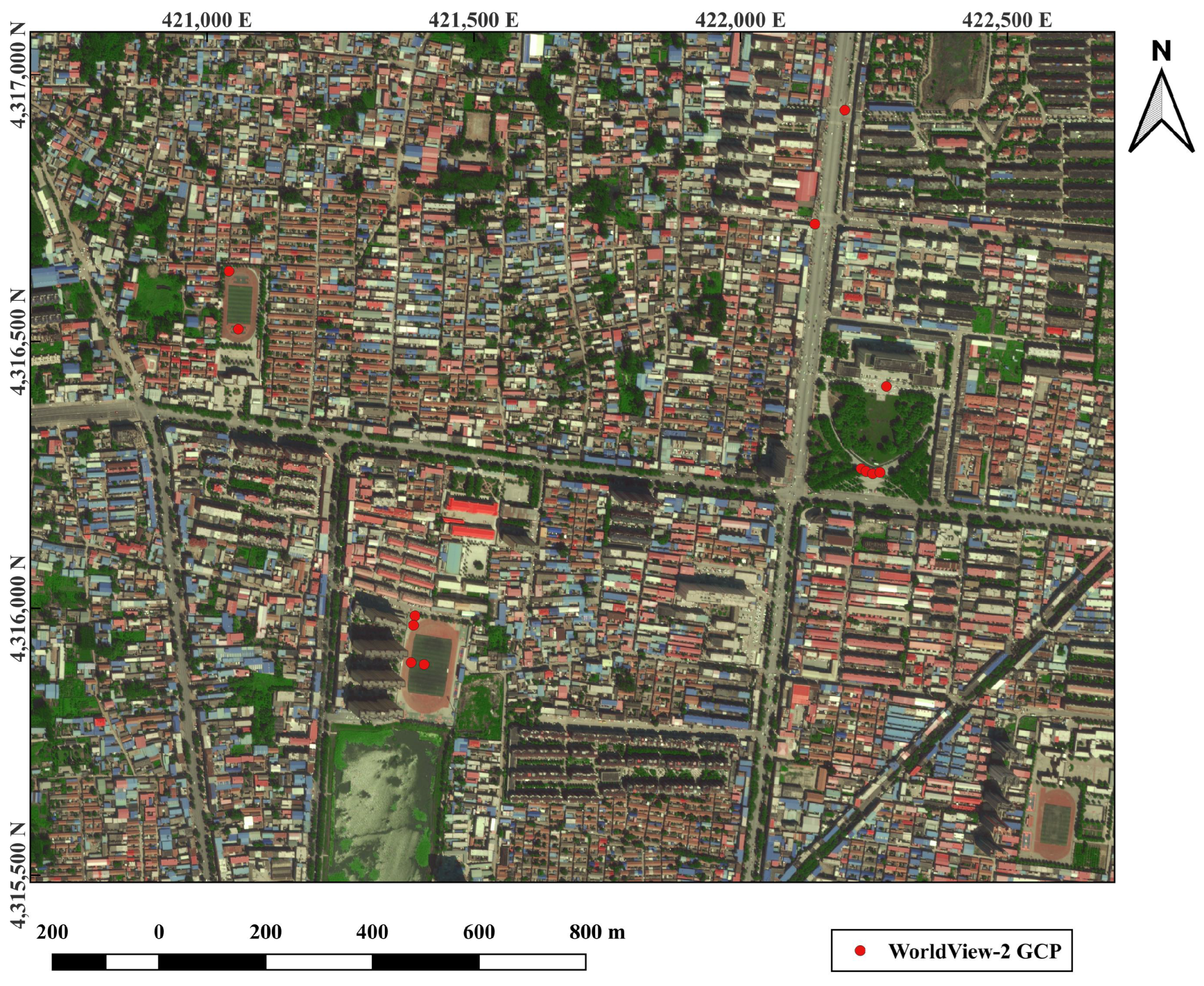
The accuracy of the reference boresight angles was validated through a comparison of the deviation in points location with the WorldView-2 image. Here, WorldView-2 imagery was used as the reference image, and 13 feature points were manually selected as GCPs. We mainly chose the corner points located on the ground as GCPs, and the distribution of GCPs was shown in Figure 10. The accuracy was shown in

Table 10. Statistics of deviation in points location comparing with the WorldView-2 image. $RMS{E}_D$ is calculated according to Equation (15).

	RMSE${}_{\mathit{X}}$±STD(m)	RMSE${}_{\mathit{Y}}$±STD(m)	RMSE${}_{\mathit{D}}$±STD(m)
After Calibration	$0.16\pm 0.16$	$0.42\pm 0.29$	$0.5\pm 0.26$

.

$$RMS{E}_D=\sqrt{(\sum _{i=1}^N{(x_{data}^i-x_{gcp}^i)}^2+{(y_{data}^i-y_{gcp}^i)}^2)/N}$$

(15)

With reference boresight angles, we triangulated the features and obtained their 3D locations. In order to compare the accuracy of the methods in the absence of GCPs, we utilized uncorrected POS data for subsequent analyses. The statistics of features’ elevation in EGM96 Geoid and relative histograms are shown in Figure 11.

The mean and standard deviation of the outcomes obtained by various techniques in Table 5 were analyzed and compared in

Table 11. Means and standard deviations of calibration results for different methods on different DEM datasets.

Method	Means (mrad)	Difference (mrad)	STD (urad)
Absolute(AW3D30)	(−3.1,−0.31,−5.78)	(−0.26,0.03,0.02)	(254,20,22)
Absolute(SRTM-GL1)	(−3.12,−0.31,−5.78)	(−0.28,0.03,0.02)	(270,20,24)
Absolute(GDEM V3)	(−2.94,−0.32,−5.77)	(−0.1,0.02,0.03)	(117,19,23)
MPE	(−2.92,−0.32,−5.78)	(−0.08,0.02,0.02)	(77,16,32)
Proposed(AW3D30)	(−2.88,−0.32,−5.77)	(−0.04,0.02,0.03)	(22,12,22)
Proposed(SRTM-GL1)	(−2.88,−0.32,−5.77)	(−0.04,0.02,0.03)	(28,12,22)
Proposed(GDEM V3)	(−2.86,−0.32,−5.76)	(−0.02,0.02,0.04)	(52,12,27)

. The groups (1,3), (1,4), (3,4), and (1,3,4) were not considered in the proposed approach because the groups having the same flight direction can lead to unavoidable errors. The findings presented in Table 11 indicate that the proposed method yields the highest precision.

5. Discussion

This study explores the use of relative height data from DEM datasets to improve the accuracy of boresight calibration in large-area aerial remote sensing imagery, with a focus on the roll angle. The variability in average elevation in such imagery can lead to deviations from the ground truth, which can be mitigated by incorporating elevation data from open DEM datasets. To address the low accuracy and resolution of absolute elevation data, we employ two strategies to enhance calibration accuracy. Firstly, we utilize the coplanarity constraint to filter ground-level image points and decrease the uncertainty of the height obtained from the DEM dataset. Secondly, we incorporate relative height data into the calibration process by minimizing the reprojection error with relative height of overlapping area. This approach provides more precise constraints than the method using the averaging elevation. Furthermore, the absolute elevation error has a minor impact on our approach, as demonstrated by the consistency between the results obtained from different datasets, as presented in Table 11.

Theconfiguration of opposite flight direction between adjacent strips is a crucial factor that affects the accuracy of boresight calibration. When opposite strips are used, the global minimum exists between adjacent overlapping areas, which can serve as a good initial state for determining the correct boresight angles based on relative height data derived from DEM data. This approach involves using the midpoints of corresponding point pairs to retrieve their elevation from the DEM data. Ifthe flight direction is the same between adjacent strips, the midpoint will deviate from the true coordinates at large boresight angles, leading to inaccuracies in the calibration process.

The horizontal resolution of the DEM dataset is a critical factor that affects calibration accuracy, as it has a significant impact on the standard deviation of the DEM elevation data. While the use of relative elevation data can somewhat alleviate the dependency on the accuracy of the DEM, low-resolution DEM datasets are still observed to decrease calibration accuracy. Additionally, since the DEM datasets were generated before the AHI images, the variation in the ground targets over time can adversely affect the calibration accuracy, as seen in Figure 6 and Figure 7. Combining high-precision 3D point cloud data with calibration could be a promising approach to further improve accuracy.

6. Conclusions

This study proposes a method for improving the accuracy of AHI boresight calibration by utilizing relative height data from open DEM datasets and applying a coplanarity constraint. Our findings highlight the potential of using low-horizontal-resolution DEM datasets for high-resolution AHI boresight calibration. In particular, we show that optimization with relative height leads to higher accuracy than optimization with absolute elevation, especially when using low-horizontal-resolution DEM datasets. The coplanarity constraint is applied to extract features with similar elevation, which are, subsequently, used in the optimization process. Experimental results on an aerial imagery dataset captured by AMMIS and three open DEM datasets validate the effectiveness of our proposed method.

References

1. Bioucas-Dias, J.M.; Plaza, A.; Camps-Valls, G.; Scheunders, P.; Nasrabadi, N.; Chanussot, J. Hyperspectral remote sensing data analysis and future challenges. IEEE Geosci. Remote Sens. Mag. 2013, 1, 6–36. [Google Scholar] [CrossRef]
2. Lu, B.; Dao, P.D.; Liu, J.; He, Y.; Shang, J. Recent advances of hyperspectral imaging technology and applications in agriculture. Remote Sens. 2020, 12, 2659. [Google Scholar] [CrossRef]
3. Wang, C.; Liu, B.; Liu, L.; Zhu, Y.; Hou, J.; Liu, P.; Li, X. A review of deep learning used in the hyperspectral image analysis for agriculture. Artif. Intell. Rev. 2021, 54, 5205–5253. [Google Scholar] [CrossRef]
4. Gebbers, R.; Adamchuk, V.I. Precision agriculture and food security. Science 2010, 327, 828–831. [Google Scholar] [CrossRef] [PubMed]
5. Su, H.; Yao, W.; Wu, Z.; Zheng, P.; Du, Q. Kernel low-rank representation with elastic net for China coastal wetland land cover classification using GF-5 hyperspectral imagery. ISPRS J. Photogramm. Remote Sens. 2021, 171, 238–252. [Google Scholar] [CrossRef]
6. Vali, A.; Comai, S.; Matteucci, M. Deep learning for land use and land cover classification based on hyperspectral and multispectral earth observation data: A review. Remote Sens. 2020, 12, 2495. [Google Scholar] [CrossRef]
7. Pahlevan, N.; Smith, B.; Binding, C.; Gurlin, D.; Li, L.; Bresciani, M.; Giardino, C. Hyperspectral retrievals of phytoplankton absorption and chlorophyll-a in inland and nearshore coastal waters. Remote Sens. Environ. 2021, 253, 112200. [Google Scholar] [CrossRef]
8. Niroumand-Jadidi, M.; Bovolo, F.; Bruzzone, L. Water quality retrieval from PRISMA Hyperspectral images: First experience in a turbid lake and comparison with Sentinel-2. Remote Sens. 2020, 12, 3984. [Google Scholar] [CrossRef]
9. Veraverbeke, S.; Dennison, P.; Gitas, I.; Hulley, G.; Kalashnikova, O.; Katagis, T.; Kuai, L.; Meng, R.; Roberts, D.; Stavros, N. Hyperspectral remote sensing of fire: State-of-the-art and future perspectives. Remote Sens. Environ. 2018, 216, 105–121. [Google Scholar] [CrossRef]
10. Kruse, F.A.; Boardman, J.W.; Huntington, J.F. Comparison of airborne hyperspectral data and EO-1 Hyperion for mineral mapping. IEEE Trans. Geosci. Remote Sens. 2003, 41, 1388–1400. [Google Scholar] [CrossRef]
11. Zhong, Y.; Hu, X.; Luo, C.; Wang, X.; Zhao, J.; Zhang, L. WHU-Hi: UAV-borne hyperspectral with high spatial resolution (H2) benchmark datasets and classifier for precise crop identification based on deep convolutional neural network with CRF. Remote Sens. Environ. 2020, 250, 112012. [Google Scholar] [CrossRef]
12. Turner, D.; Lucieer, A.; Wallace, L. Direct georeferencing of ultrahigh-resolution UAV imagery. IEEE Trans. Geosci. Remote Sens. 2013, 52, 2738–2745. [Google Scholar] [CrossRef]
13. Benassi, F.; Dall’Asta, E.; Diotri, F.; Forlani, G.; Morra di Cella, U.; Roncella, R.; Santise, M. Testing accuracy and repeatability of UAV blocks oriented with GNSS-supported aerial triangulation. Remote Sens. 2017, 9, 172. [Google Scholar] [CrossRef]
14. He, F.; Zhou, T.; Xiong, W.; Hasheminnasab, S.M.; Habib, A. Automated aerial triangulation for UAV-based mapping. Remote Sens. 2018, 10, 1952. [Google Scholar] [CrossRef]
15. Forlani, G.; Diotri, F.; Cella, U.M.d.; Roncella, R. Indirect UAV strip georeferencing by on-board GNSS data under poor satellite coverage. Remote Sens. 2019, 11, 1765. [Google Scholar] [CrossRef]
16. Štroner, M.; Urban, R.; Seidl, J.; Reindl, T.; Brouček, J. Photogrammetry using UAV-mounted GNSS RTK: Georeferencing strategies without GCPs. Remote Sens. 2021, 13, 1336. [Google Scholar] [CrossRef]
17. Queally, N.; Ye, Z.; Zheng, T.; Chlus, A.; Schneider, F.; Pavlick, R.P.; Townsend, P.A. FlexBRDF: A flexible BRDF correction for grouped processing of airborne imaging spectroscopy flightlines. J. Geophys. Res. Biogeosci. 2022, 127, e2021JG006622. [Google Scholar] [CrossRef]
18. Hartley, R.; Zisserman, A. Multiple View Geometry in Computer Vision; Cambridge University Press: Cambridge, UK, 2003. [Google Scholar]
19. Lowe, D.G. Object recognition from local scale-invariant features. In Proceedings of the Seventh IEEE International Conference on Computer Vision, Corfu, Greece, 20–27 September 1999; Volume 2, pp. 1150–1157. [Google Scholar]
20. Lowe, D.G. Distinctive image features from scale-invariant keypoints. Int. J. Comput. Vis. 2004, 60, 91–110. [Google Scholar] [CrossRef]
21. Bay, H.; Ess, A.; Tuytelaars, T.; Van Gool, L. Speeded-up robust features (SURF). Comput. Vis. Image Underst. 2008, 110, 346–359. [Google Scholar] [CrossRef]
22. Rublee, E.; Rabaud, V.; Konolige, K.; Bradski, G. ORB: An efficient alternative to SIFT or SURF. In Proceedings of the 2011 International Conference on Computer Vision, Barcelona, Spain, 6–13 November 2011; pp. 2564–2571. [Google Scholar]
23. Park, F.C.; Martin, B.J. Robot sensor calibration: Solving AX= XB on the Euclidean group. IEEE Trans. Robot. Autom. 1994, 10, 717–721. [Google Scholar] [CrossRef]
24. Tsai, R.Y.; Lenz, R.K. A new technique for fully autonomous and efficient 3 d robotics hand/eye calibration. IEEE Trans. Robot. Autom. 1989, 5, 345–358. [Google Scholar] [CrossRef]
25. Gupta, R.; Hartley, R.I. Linear pushbroom cameras. IEEE Trans. Pattern Anal. Mach. Intell. 1997, 19, 963–975. [Google Scholar] [CrossRef]
26. Muller, R.; Lehner, M.; Muller, R.; Reinartz, P.; Schroeder, M.; Vollmer, B. A program for direct georeferencing of airborne and spaceborne line scanner images. Int. Arch. Photogramm. Remote Sens. Spat. Inf. Sci. 2002, 34, 148–153. [Google Scholar]
27. Lenz, A.; Schilling, H.; Perpeet, D.; Wuttke, S.; Gross, W.; Middelmann, W. Automatic in-flight boresight calibration considering topography for hyperspectral pushbroom sensors. In Proceedings of the 2014 IEEE Geoscience and Remote Sensing Symposium, Quebec City, QC, Canada, 13–18 July 2014; pp. 2981–2984. [Google Scholar]
28. Fletcher, R. A Modified Marquardt Subroutine for Non-Linear Least Squares; Atomic Energy Authority Research Group: Harwell, UK, 1971. [Google Scholar]
29. Habib, A.; Zhou, T.; Masjedi, A.; Zhang, Z.; Flatt, J.E.; Crawford, M. Boresight calibration of GNSS/INS-assisted push-broom hyperspectral scanners on UAV platforms. IEEE J. Sel. Top. Appl. Earth Obs. Remote Sens. 2018, 11, 1734–1749. [Google Scholar] [CrossRef]
30. Skaloud, J.; Lichti, D. Rigorous approach to bore-sight self-calibration in airborne laser scanning. ISPRS J. Photogramm. Remote Sens. 2006, 61, 47–59. [Google Scholar] [CrossRef]
31. de Oliveira Junior, E.M.; Dos Santos, D.R. Rigorous calibration of UAV-based LiDAR systems with refinement of the boresight angles using a point-to-plane approach. Sensors 2019, 19, 5224. [Google Scholar] [CrossRef]
32. Tadono, T.; Shimada, M.; Murakami, H.; Takaku, J. Calibration of PRISM and AVNIR-2 onboard ALOS “Daichi”. IEEE Trans. Geosci. Remote Sens. 2009, 47, 4042–4050. [Google Scholar] [CrossRef]
33. Takaku, J.; Tadono, T.; Tsutsui, K. Generation of High Resolution Global Dsm from Alos Prism. ISPRS Ann. Photogramm. Remote Sens. Spat. Inf. Sci. 2014, 2. [Google Scholar] [CrossRef]
34. Remote Sensing Technology Center of Japan. AW3D: Global High-Resolution 3D Map. Available online: https://www.restec.or.jp/en/solution/aw3d.html (accessed on 22 April 2023).
35. Yamaguchi, Y.; Kahle, A.B.; Tsu, H.; Kawakami, T.; Pniel, M. Overview of advanced spaceborne thermal emission and reflection radiometer (ASTER). IEEE Trans. Geosci. Remote Sens. 1998, 36, 1062–1071. [Google Scholar] [CrossRef]
36. NASA Jet Propulsion Laboratory (JPL). NASA Shuttle Radar Topography Mission Global 1 Arc Second, 2013. Type: Dataset. Available online: https://lpdaac.usgs.gov/products/srtmgl1v003/ (accessed on 22 April 2023).
37. Rosenqvist, A.; Shimada, M.; Ito, N.; Watanabe, M. ALOS PALSAR: A pathfinder mission for global-scale monitoring of the environment. IEEE Trans. Geosci. Remote Sens. 2007, 45, 3307–3316. [Google Scholar] [CrossRef]
38. ASF. ALOS PALSAR—Radiometric Terrain Correction. Type: Dataset. Available online: https://asf.alaska.edu/data-sets/derived-data-sets/alos-palsar-rtc/alos-palsar-radiometric-terrain-correction/ (accessed on 22 April 2023).
39. Tadono, T.; Nagai, H.; Ishida, H.; Oda, F.; Naito, S.; Minakawa, K.; Iwamoto, H. Generation of the 30 M-mesh global digital surface model by ALOS PRISM. Int. Arch. Photogramm. Remote Sens. Spat. Inf. Sci. 2016, 41. [Google Scholar] [CrossRef]
40. JAXA. AW3D30 DSM Data Map. Available online: https://www.eorc.jaxa.jp/ALOS/en/aw3d30/data/index.htm (accessed on 22 April 2023).
41. Gesch, D.; Oimoen, M.; Danielson, J.; Meyer, D. Validation of the ASTER global digital elevation model version 3 over the conterminous United States. Int. Arch. Photogramm. Remote Sens. Spat. Inf. Sci. 2016, 41, 143. [Google Scholar] [CrossRef]
42. Geospatial Data Cloud. Available online: http://www.gscloud.cn (accessed on 22 April 2023).
43. Rodriguez, E.; Morris, C.S.; Belz, J.E. A global assessment of the SRTM performance. Photogramm. Eng. Remote Sens. 2006, 72, 249–260. [Google Scholar] [CrossRef]
44. ASF Data Search. Available online: https://search.asf.alaska.edu/ (accessed on 22 April 2023).
45. Davis, J.C.; Sampson, R.J. Statistics and Data Analysis in Geology; Wiley: New York, NY, USA, 1986; Volume 646. [Google Scholar]
46. Okutomi, M.; Kanade, T. A multiple-baseline stereo. IEEE Trans. Pattern Anal. Mach. Intell. 1993, 15, 353–363. [Google Scholar] [CrossRef]
47. Fischler, M.A.; Bolles, R.C. Random sample consensus: A paradigm for model fitting with applications to image analysis and automated cartography. Commun. ACM 1981, 24, 381–395. [Google Scholar] [CrossRef]
48. Ester, M.; Kriegel, H.P.; Sander, J.; Xu, X. A density-based algorithm for discovering clusters in large spatial databases with noise. In Proceedings of the Kdd, Portland, OR, USA, 2 August 1996; Volume 96, pp. 226–231. [Google Scholar]
49. Ma, J.; Zhao, J.; Jiang, J.; Zhou, H.; Guo, X. Locality preserving matching. Int. J. Comput. Vis. 2019, 127, 512–531. [Google Scholar] [CrossRef]
50. Jiang, X.; Ma, J.; Jiang, J.; Guo, X. Robust feature matching using spatial clustering with heavy outliers. IEEE Trans. Image Process. 2019, 29, 736–746. [Google Scholar] [CrossRef]
Figure 1. Thumbnails of four experiment strips (UTM Zone 50N). The red arrows indicate the relative flight directions of the strips. These strips are indexed from north to south as the first, second, third, and fourth strips, respectively. Meanwhile, the blue rectangles denote the locations of the three calibration strips for reference. The numbers encircled indicate the indices of the strips.
Remotesensing 15 02268 g001
Figure 2. Flow chart of this study.
Remotesensing 15 02268 g002
Figure 3. The suitable features and unsuitable features in boresight calibration. (a,b) are unsuitable as they are related to height, and are averaged at the low-resolution DEM datasets. (c,d) are unsuitable due to their relationship with shadows. (eh) are suitable features that are not influenced by height or shadows.
Remotesensing 15 02268 g003
Figure 4. Schematic diagram of the projection error of feature pairs in adjacent strips. Coordinate reference system is drawn in red lines and the origin is set at O. Circles with dots or crosses denote the flight direction towards outside or inside the paper.  O a m O b m  and  O c n , and  O d n  are four optical centers of two feature pairs in their corresponding strip frames.  C a m C b m  and  C c n , and  C d n  are normalized intrinsic parameters.  P a m P b m  and  P c n P d n  are projection points in projection plane H H m  and  H n  are the true projection planes of two feature pairs. Blue lines denote the influence of perturbation on roll angle to projection lines.  θ  is the perturbation of roll angle.
Remotesensing 15 02268 g004
Figure 5. The distribution of Euclidean distance difference vector set G in different overlapping area and the related feature selection results. (ac) Feature selection results with RFM-SCAN. (df) Feature selection results with LPM method. (gi) Feature selection results with proposed method.
Remotesensing 15 02268 g005
Figure 6. Part of DEM retrieval results of cluster 1 (in Figure 5i) from three DEM datasets. (a) DEM data of SRTM-GL1. (b) DEM data of AW3D30. (c) DEM data of ASTER GDEM V3. (df) The dark blue pixel blocks are the position of the feature points in the corresponding DEM datasets. (g) The position of the feature points in the third strip image. The green marks are part of the feature points of cluster 1 in Figure 5i. The pink marks are part of the feature points of cluster 2 in Figure 5i.
Remotesensing 15 02268 g006
Figure 7. Part of DEM retrieval results of cluster 2 (in Figure 5i) from three DEM datasets. (a) DEM data of SRTM-GL1. (b) DEM data of AW3D30. (c) DEM data of ASTER GDEM V3. (df) The dark blue pixel blocks are the position of the feature points in the corresponding DEM datasets. (g) The position of the feature points in the third strip image. The green marks are part of the feature points of cluster 1 in Figure 5i. The pink marks are part of the feature points of cluster 2 in Figure 5i.
Remotesensing 15 02268 g007
Figure 8. The histograms depict the distribution of feature points across different regions and DEM datasets. Red bins represent all features, blue bins represent selected features with similar disparity, and sky-blue dotted lines represent Gaussian fitting results using the elevation data of selected features. Number 1 to 4 denote the cluster indices in Figure 5.
Remotesensing 15 02268 g008
Figure 9. The city area with 11 GCPs and overlapping area of calibration strips (UTM Zone 50N).
Remotesensing 15 02268 g009
Figure 10. The location map of GCPs in WorldView-2 image(UTM Zone 50 N).
Remotesensing 15 02268 g010
Figure 11. Elevation histograms of image features from 4 clusters in EGM96 Geoid. The elevation is triangulated with the reference boresight angles.
Remotesensing 15 02268 g011