Article

The Dynamic Heterogeneous Relationship between Urban Population Distribution and Built Environment in Xi’an, China: A Case Study

1
Key Laboratory of Urban Land Resources Monitoring and Simulation, Ministry of Natural Resources, Shenzhen 518000, China
2
School of Geography and Tourism, Shaanxi Normal University, Xi’an 710119, China
3
Academy of Digital China (Fujian), Fuzhou University, Fuzhou 350003, China
4
School of Civil and Hydraulic Engineering, Huazhong University of Science and Technology, Wuhan 430074, China
5
Shenzhen Key Laboratory of Spatial Information Smart Sensing and Services, Research Institute of Smart Cities, Shenzhen University, Shenzhen 518060, China
6
Department of Urban Informatics, School of Architecture and Urban Planning, Shenzhen University, Shenzhen 518060, China
*
Author to whom correspondence should be addressed.
Remote Sens. 2023, 15(9), 2257; https://doi.org/10.3390/rs15092257
Submission received: 21 February 2023 / Revised: 7 April 2023 / Accepted: 13 April 2023 / Published: 25 April 2023

Abstract

:
The interaction between the population and built environment is a constant topic in urban spaces and is the main driving force of urban evolution. Understanding urban population distribution and its relationship with the built environment could provide guidance for urban planning, traffic, and disaster management. Following this line of thought, this study conducted an empirical analysis in Xi’an, a rapidly developing western city in China. Well-permeated mobile phone location data were used to represent the spatiotemporal dynamics of the population, and the built environment was characterized from five perspectives—transportation, location, building, greenery, and land use—using multisource geospatial data. Finally, the dynamic heterogeneous influence of built environment factors on population distribution was examined using multiscale geographically weighted regression (MGWR). Overall, the influencing coefficients exhibited a significant dynamic changing process from a temporal perspective and simultaneously demonstrated spatial nonstationarity. Moreover, the specific findings about the influence of each built environment factor facilitate a deeper insight into dynamic population distribution and its determinants.

1. Introduction

The interaction between the built environment and population distribution has long been a topic of discussion in the fields of urban planning and geography. The spatial distribution of facilities or land use in urban space is the internal motivation of human mobility, which generates an effect on human spatial distribution. An understanding of human distribution can provide guidance for the planning and allocation of urban facilities. Therefore, an investigation of the relationship between population distribution and the built environment would provide immediate benefits to urban planning, as well as effective support for urban traffic and disaster emergency management, such as in the case of floods or infectious diseases, promoting sustainable urban development [1,2,3,4].
Until recently, accessing high-resolution population data has been difficult, and traditional survey methods can only collect population distribution data at the scale of administrative units. Fortunately, the recent emergence of big geospatial data has led to the use of mobile phones as sensors for collecting information on human activity. Compared with traditional survey data, this type of big data, mainly including mobile phone and social media data, can not only include large numbers of people but also possess fine spatial and temporal resolution, which provides great opportunities for understanding human dynamics and their interaction with urban spaces [5,6,7,8]. As a proxy for human activity, big sensing data have been extensively utilized to investigate population distribution and its relationship with the built environment. In general, the related studies can be summarized into two threads.
The first focuses on estimating the fine-resolution population distribution. The open-access population distribution data are rough in spatial and temporal scales and ignore temporal dynamic (e.g., hourly dynamic) changes in population distribution. To fill this gap, some studies have attempted to map population data with high spatial and temporal resolutions by integrating machine learning techniques with multisource data. For instance, the geospatial data, e.g., land use, remotely sensed data, point of interest (POI), building, and roads are used to measure the built environment; then, the characteristics of the built environment are considered as weight or predictive variables to transform population data from the survey administrative unit to predetermined high-resolution spatial units, e.g., grid cells [9,10,11,12,13,14,15]. Moreover, using mobile phone data as population data, neural network-related methods have been utilized to model the spatial and temporal dependency of populations to map dynamic population [16,17,18,19,20]. However, these black box methods cannot reveal the intrinsic relationship between the built environment and population distribution.
The second research community focused on uncovering the influence of the built environment on population distribution. After reviewing existing literature, it was found that urban vibrancy is a theme frequently investigated in related studies. Since the concept was first proposed by Jacobs [21], urban vibrancy has been a long-standing concern in urban planning, and it has been emphasized that vibrant streets should attract a large number of people engaged in diverse activities [22]. Therefore, urban vibrancy is a significant indicator of habitability, and is closely associated with the design of urban built environments [23]. Likewise, the newly available geosensing big data allow researchers to re-examine the dynamics of urban vibrancy at an unprecedented spatial and temporal scale [24]. These studies extracted population distribution from mobile phones or social media data to quantify urban vibrancy, and subsequently explored the spatiotemporal variation of urban vibrancy and its relationship with built environment factors [25,26,27,28,29,30,31,32,33]. It could be seen that most of these empirical analyses were conducted in a Chinese context and were mainly concentrated on three well-developed and highly dense cities, namely, Beijing, Shanghai and Shenzhen, while the findings about developing cities are scarce. However, other cities are experiencing rapid development in contemporary China, leading to a population explosion and a renewal of the built environment (e.g., urban village renovation). Therefore, it is necessary to examine the interaction between population distribution and built environment in a developing urban context, and more empirical findings should be identified in a timely manner to guide urban planning and renewal.
Using Xi’an, a rapidly developing city in western China, as a case study, Li et al. [34] analyzed the spatiotemporal distribution characteristics and mechanism of urban population density using a Baidu heat map and POI data. Although the results provide an understanding of urban population distribution, there are still two drawbacks that could be addressed. First, administrative districts (only 50 subdistricts) were used as spatial analysis units, which are too rough a scale for obtaining abundant knowledge about population distribution. However, the advantage of geospatial big data is that it enables us to inspect urban spaces at a more microcosmic spatial and temporal scale. Second, only the global relationship was examined using ordinary least squares (OLS) models in the above study. However, there is an obvious spatial and temporal heterogeneity when the population distribution interacts with the built environment [13,32]. In particular, the influence of the built environment on population distribution shows a significant spatial non-stationary characteristic.
To fill this gap, this study takes Xi’an as the study area and aims to investigate the dynamic heterogeneous relationship between population distribution and the built environment. Specifically, the high permeability of mobile phone location data was used as a proxy for urban population data, which were then grouped into street blocks generated from urban roads to represent population distribution. Multisource data were used to quantify the built environments of street blocks from five perspectives: transportation, location, buildings, greenery, and land use. Finally, multiscale geographically weighted regression was used to identify the dynamic heterogeneous influence of built environment factors on urban population distribution. The results are expected to enrich the existing literature by deepening our understanding of the determining mechanisms of dynamic urban population distribution.

2. Materials

2.1. Study Area

The experimental analysis was conducted in Xi’an, China (Figure 1a). As a famous ancient capital, Xi’an has a long history and abundant Chinese culture, making it a distinguished tourist destination. Xi’an is the largest city in northwest China and is an important national base for scientific research, education, and industry; it is also one of the nine central cities of China. According to the seventh national census (2020), the city has a total population of more than 12.9 million and covers 13 administrative districts (a total area of 10.108 km2), including 6 downtown, 4 suburban, and 3 rural districts (Figure 1b). This study selected areas within an urban freeway as the study area (Figure 1c) because the collected heat map data only covers the area within the freeway, which is also a well-developed central urban area and covers most of the population and facilities; therefore, the area could be as a representative of exploring relationship between human distribution and built environment.
The selection of spatial analysis units has long been debated in the study of human dynamics and population distribution. Recently, different spatial analysis units (regular grid cells, hexagonal cells, and traffic analysis zones) have been utilized to investigate urban human mobility and discover valuable knowledge [22,25]. It is difficult to avoid and eliminate the effect of spatial analysis units on the results of a geographical analysis, which is denoted as the modifiable areal unit problem (MAUP). In urban circumstances, the road network can be considered an artery of a city and connects different areas of the city. The road network divides the entire city into different street blocks. These street blocks are enveloped by road lines and can be used for spatial analysis [35]. Therefore, referring to the method in the literature [36], this study utilized the urban road network from OpenStreetMap to generate 859 street blocks as spatial analysis units (Figure 1).

2.2. Dataset

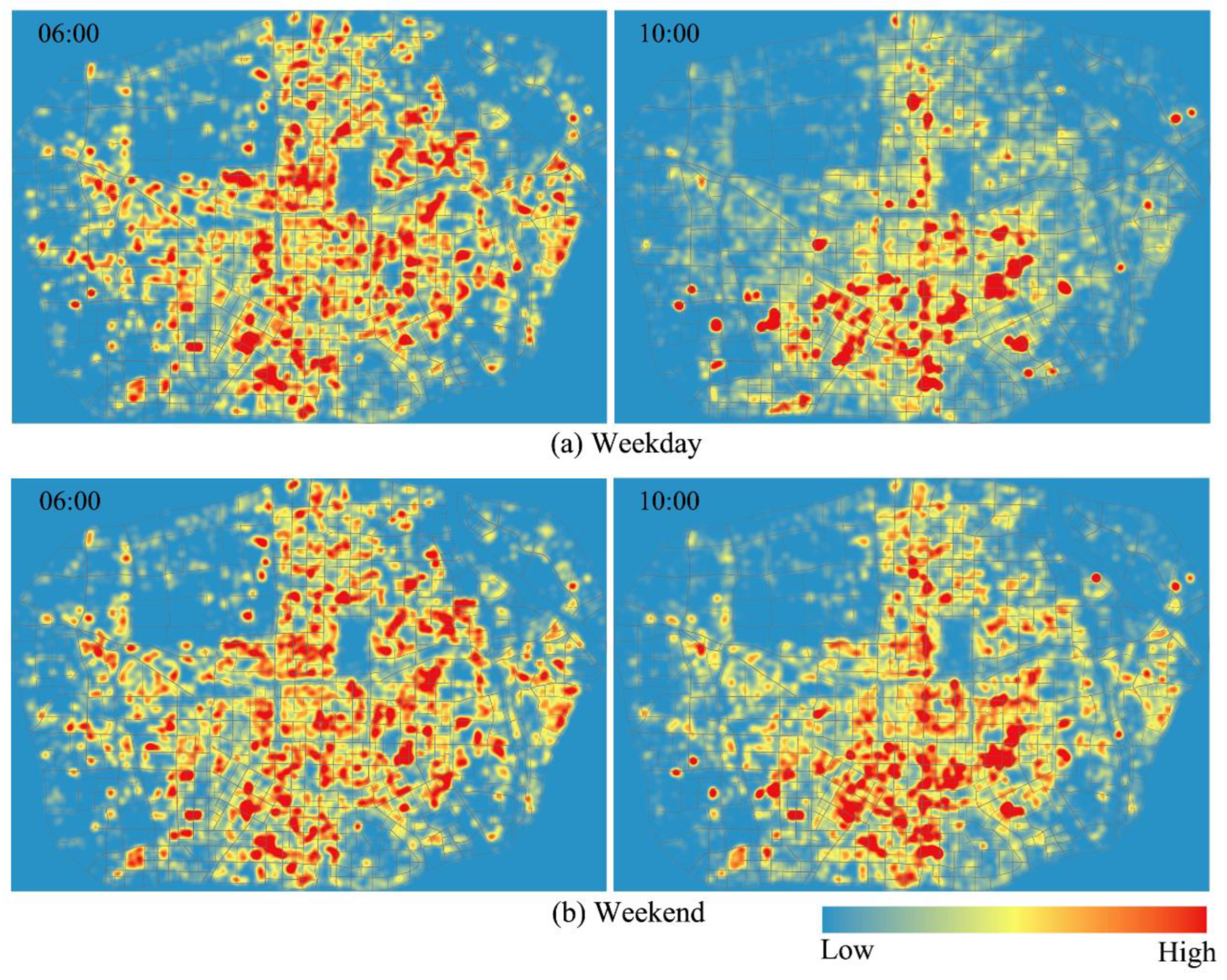
The population dataset was collected from a popular social media app (WeChat), which had more than 10 billion Chinese subscribers in 2018 and included different age groups. This app provides a travel-related function that allows residents to check how crowded their own neighborhoods are (https://heat.qq.com/index.php, accessed on 21 February 2023). It displays the urban human spatial distribution using a heatmap produced by the user’s real-time location, which has been introduced to investigate the spatiotemporal dynamics of urban populations [13,34]. Based on the heat map, population distribution data can be obtained from the background of the app. The collected population data are in the form of a dot matrix with a spatial resolution of approximately 25 m. The attributes of each dot include longitude, latitude, count, and sample time. However, the count does not represent the real number of people, but a normalized, relative value that indicates the intensity of population distribution, and a larger value indicates a greater population around the dot. One typical workday (10 October 2019) and one weekend day (12 October 2019) were obtained to compare the differences in population distribution between workdays and weekends. We collected diurnal population data from the early morning (06:00 a.m.) to midnight (24:00 p.m.) at two hours intervals obtaining a total of ten time periods for each day. The kernel density of the human distribution at 06:00 a.m. and 10:00 a.m. on weekdays and weekends was also assessed (Figure 2). The population distribution at 06:00 a.m. is more spatially dispersive than that observed at 10:00 am on a weekday, because workplaces are more concentrated in spatial distribution than residential places. In contrast, the population distribution on weekends is more spatially dispersive than on weekdays at 10:00 a.m., because residents do not work on weekends. This demonstrated that the spatial distribution of residents changed over time, generating a dynamic spatiotemporal scenario.
The road network data used in this study were obtained from OpenStreetMap, and the building footprint data and POI were collected from the popular online map service Gaode (https://www.amap.com, accessed on 21 February 2023).

3. Methodology

3.1. Population Density and Built Environment Factors

The street blocks were adopted as spatial analysis units; thus it is necessary to aggregate these sample dot-matrix population data into street blocks. Therefore, the population density of street-block i at time period t could be calculated using:
D i t = k = 1 N c o u n t i t A i ,
where D i t represents the population density of street block i at time period t , N represents the total number of dots within the street block i , and A i represents the street block area. Population density was used as the response variable in regression analysis.
For the independent variables, we quantified the urban built environment from six perspectives: transportation, location, building footprint, normalized difference vegetation index (NDVI), and land use (Table 1). For transportation, we used road interaction and density to represent the urban design within street blocks and bus stops, and the distance to the nearest subway station represented the convenience of public transport. The location of the street block indicates the distance from the unit to the urban center, which could also play an important role in population distribution. In terms of building footprint, the building coverage and floor area ratios were selected to denote the building density and intensity of the street block, respectively. In addition, the NDVI extracted from Landsat 8 was used to indicate greenery within street blocks. In terms of land use, POIs can represent the land function of street blocks; thus, different types of POI densities (commercial, residential, industrial, and public) are calculated to determine the functional characteristics of the block. Entropy was employed to quantify the mixture of different types of POI within a street block. In total, 14 independent variables were used to describe the characteristics of the built environments of the street blocks.

3.2. Regression Analysis

Global and local regression models were employed to investigate the relationship between built environment and population distribution. The multiple linear regression model (MLR) was used to execute the global static regression analysis, which assumes that the independent variables across whole space have the same influence on the dependent variables; thus, only one coefficient could be estimated for each independent variable over all spatial units. The formula for the global regression model was as follows:
Y i = β 0 + j β j x i j + ε i
where Y i is the population density of street block i , and x i j represents the j independent variable at street block i . β j is the global estimated coefficient for the built environment variables, β 0 represents the estimated constant and ε i represents the corresponding residual.
However, the distribution of geographical elements shows characteristics of spatial heterogeneity, and the influence of independent variables on the dependent variable is spatial nonstationary, which means that the same built environment variable at different urban locations would generate different effects on population distribution. Geographically weighted regression (GWR) and its modified models were proposed to quantify the spatially varying influence of independent variables on dependent variables by embedding the spatial location of the samples. This study utilizes a multiscale geographically weighted regression (MGWR) model to derive the spatiotemporal influencing mechanism of the built environment on population distribution. Compared with traditional GWR, the MGWR model relaxes the assumption that the spatially varying processes of all elements in a GWR model have the same spatial scale or bandwidth, allowing for the optimization of covariate-specific bandwidths for conditional relationships between the response variables and different predictor variables, which significantly improves the GWR model [37]. The MGWR model is formulated as follows:
Y i = β b w 0 ( u i , v i ) + j β b w j ( u i , v i ) X i j + ε i
where b w j in β b w j represents the specific optimal bandwidth for the calibration of the j th conditional relationship, and β b w 0 represents the estimated constant, ( u i , v i ) represents the central location of street block i and Y i is the population density of street block i , and X i j represents the j independent variable at street block i . The specific fitting process of coefficients was performed according to Fotheringham [37]; the MGWR2.2 software (https://sgsup.asu.edu/sparc/multiscale-gwr, accessed on 21 February 2023) was employed to estimate the spatial varying coefficients of built environment.

3.3. Dynamic Influence of Built Environment on Human Distribution

The MGWR model was implemented to quantify the spatially varying influence of the built environment on population distribution for each time period, and there were a total of ten time periods; therefore, there were ten estimated coefficients for each street block during the daytime. Here, β i j t denotes the regression coefficient of the j th built environment variable at street block i during the time period t . For all street blocks, the influence of the j th built environment variable can be described as a two-dimensional matrix as follows:
β j = β 1 j t 1 , β 1 j t 2 , , β 1 j t 10 β 2 j t 1 , β 2 j t 2 , , β 2 j t 10 β n j t 1 , β n j t 2 , , β n j t 10
where n is the total number of street blocks ( n = 859), and β j represents the dynamic change in the influence of the j th built environment variable on the population distribution during the daytime for all street blocks. The row vector β i j = [ β i j t 1 , β i j t 2 , , β i j t 10 ] indicates the temporal change in the influence of the j th built environment variable on the population distribution at the street block i . The column vector β j t = [ β 1 j t , β 2 j t , , β n j t ] T indicates the spatial variation in coefficients for all street blocks during t .

4. Results

4.1. Global Static Relationship between Population Distribution and Built Environment

The MLR model was first used to estimate the global static relationship between the built environment and population density. For the dependent variable, we summed the count of all time periods and then divided it by the area of the street block to represent population density. A multicollinearity test was implemented before the regression analysis and variables with VIF (variance inflation factor) greater than 10. Consequently, the POI density was removed, and the remaining 13 variables were input into the MLR model.
Table 2 shows the regression results for MLR. In general, the proposed independent variables could explain approximately 52.1% and 60.4% of the population density of street blocks on weekdays and weekends, respectively.
The results of the MLR model indicated that built environment factors could better explain the population distribution on weekends. For a transport-related built environment, neither road density nor bus station density demonstrated a significant relationship with population distribution, while the number of road interactions increased population distribution within street blocks on both weekdays and weekends. For subway stations, a significant negative relationship with population distribution was detected on weekdays and weekends. As discussed in [14], the construction of a subway greatly improves the traffic accessibility of street blocks, promoting the gathering of resources, such as businesses, residences, and jobs, leading to a denser population distribution in the relevant street blocks.
When considering building footprints, a higher building coverage ratio may lead to a smaller population distribution, which is consistent with the literature [13]. One possible reason for this is that some street blocks located at the edge of the city are covered by industrial parks and villages, and these blocks usually have large building coverage but a low population density. Similar to a previous study [38], a high FAR indicates that there are more high-rise buildings within street blocks, which generates a dense population distribution.
Commercial facilities attract residents, especially on weekends. The significant positive correlation shown between residential POI and population distribution was stronger on weekends because most residents were likely participating in activities in or near their homes. Industrial POI promotes an increase in population density on weekdays, while an inhibitory relationship was detected on weekends. Street blocks with public facilities such as schools, governments, and hospitals, are more attractive to people, such as students and staff on weekdays than on weekends. When considering land use mixture, no significant relationship was observed between the POI mixture and population distribution on both weekdays and weekends, which is inconsistent with previous literature [34]. It still needs to be further investigated whether the scale of the spatial analysis unit has an effect on the regression results of the land use mixture.
In city, the high NDVI street blocks are covered by some parks; these areas are usually sparsely populated. Thus, an increase in NDVI in a street block reduces the population density within the block [14]. The lack of a linearly significant relationship with the population distribution in terms of the location of street blocks can be attributed to the following factor: the city has undergone a transformation from an early monocentric spatial structure to a polycentric one, especially over the past two decades. Therefore, the spatial distribution of facilities and populations is more dispersive than it was in previous times when the city was monocentric in structure.

4.2. Local and Dynamic Relationship between Population Density and Built Environment

This study utilized Moran’s I index to check the spatial autocorrelation of urban population distribution. The average Moran’s I values on weekdays and weekends were 0.287 and 0.326, respectively (Figure 3a). The imbalance of urban resources and facilities results in an unevenly distributed population that shows heterogeneous characteristics in urban spaces [32,39]. In other words, the population distribution of one street block is correlated with that of its surrounding street blocks, which can be measured using spatial autocorrelation. The average Moran’s I values on weekdays and weekends indicated that the population distribution showed remarkable spatial aggregation for all time periods. This significant spatial heterogeneity necessitates considering the spatial location of street blocks when quantifying the relationship between population distribution and built environment.
The temporal change in the goodness of fit of the MGWR model was investigated (Figure 3b). Table 3 and Table 4 show the summary statistics of regression of MGWR on weekday and weekend, respectively. Compared to the global regression model, it could be seen that both the AIC and adjusted R2 have a significant improvement, which was achieved by considering spatial heterogeneity characteristics when examining the relationship between the built environment and population distribution. The average of adjusted R2 on weekdays and weekends were 0.61 and 0.72, respectively. Similarly, the built environment variable better explained the dynamics of population distribution on weekends than on weekdays. The goodness of fit undergoes a “fist fall after rise” process over time periods on weekdays while a “overall steady decrease” tendency is observed on weekends. On workdays, commuting activities are predominant, and most residents need to attend urban workplaces during the daytime, which leads to large fluctuations in human spatiotemporal distribution.
Based on the results of the MGWR model, we checked the significance of each built environment variable for all periods and found that eight variables satisfied the significance test on both workdays and weekends: subway, BCR, FAR, NDVI, CPOI, RPOI, IPOI, PPOI. Unlike the global relationship, the road interaction (RI) does not significantly influence the population density of street blocks at the local scale. For each significant variable, the regression coefficients were organized as a two-dimensional matrix. It is difficult to visualize temporally and spatially varying coefficients simultaneously; thus, we explain the temporal and spatial characteristics of the coefficients separately. From a temporal perspective, the median of each column vector in the coefficient matrix was utilized to reveal the temporal dynamic variation of the coefficients for each built environment variable. For spatial characteristics, the median of each row vector in the coefficient matrix was used to present the spatially varying influence of each built environment variable on population distribution.

4.2.1. Temporal Dynamic Relationship between Built Environment and Population Distribution

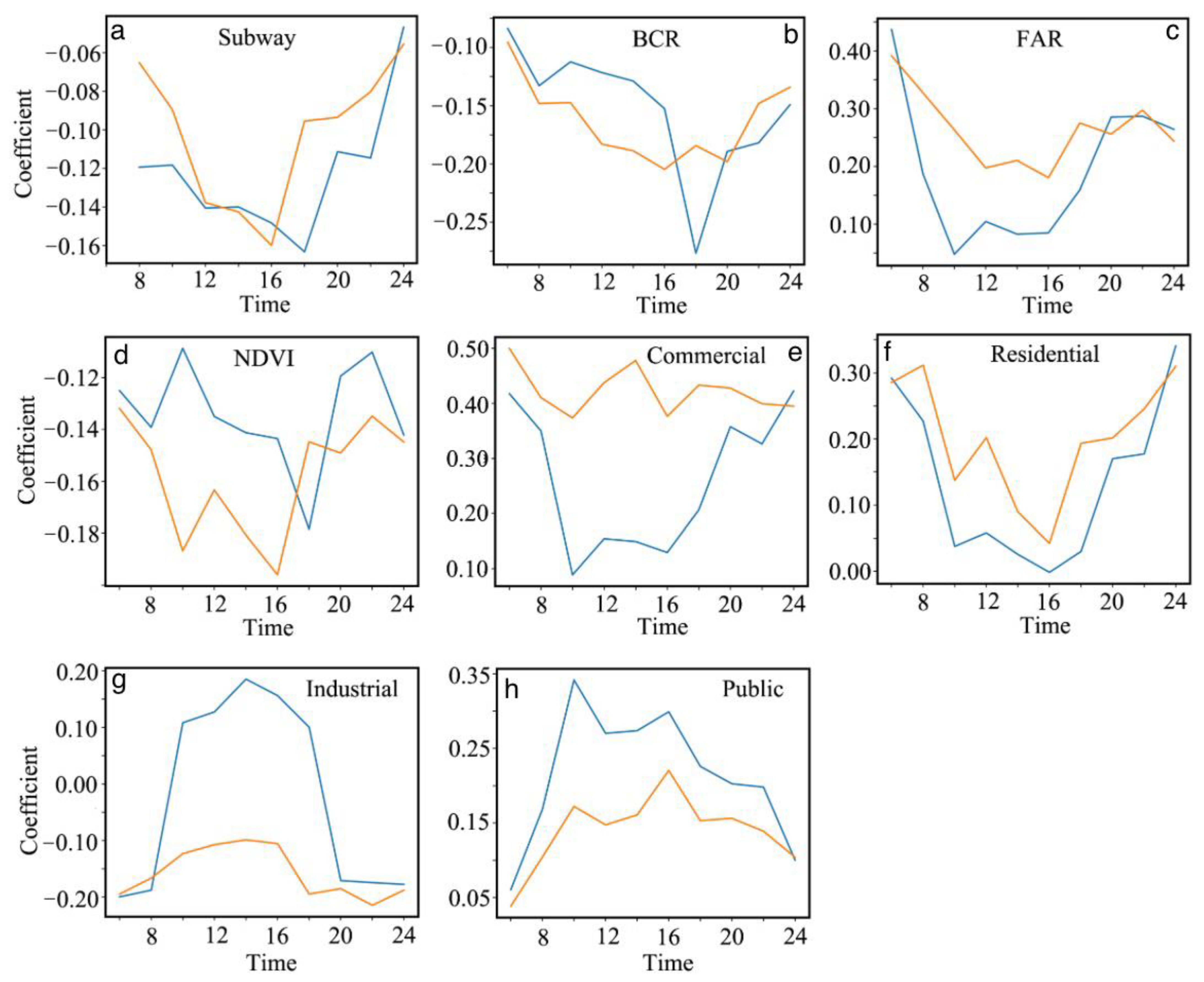
The dynamic changes over time in eight significant built environment variables are shown in Figure 4. The distance to nearest subway station played a negative role on population distribution of street blocks during all time periods, which first increased and then decreased. This may be caused by commuting activities on workdays, in which many residents take the subway home after work. Similarly, a negative relationship was detected on BCR for all time periods on both weekdays and weekends, and a sharp trough also occurred at the evening commuting peak, strengthening the link between commuting activity and a large variation in urban population distribution on workdays. Another attribute of the building footprint, FAR has a positive effect on the population density of blocks for all time periods and a similar dynamic curve on both workdays and weekends. In fact, urban residential areas are filled with high-rise buildings in Xi’an, which results in a high FAR in residential communities, and residents are likely to engage in activities near their homes on weekends; thus, the population density is higher within these high-FAR residential communities on weekends than on weekdays.
The inhibitory effect of NDVI on population density is stronger on weekends than that observed during the week, and the fluctuations occurring at the travel peak indicated that residents’ travel rhythms could result large shifts in the influencing strength of this variable.
Regarding land-use-related variables, work-related activities affect CPOIs in that the influence is weak during work hours, whereas it maintains a high positive influence on population density because residents are likely to engage in commercial activities, such as shopping, catering, and entertainment on weekends. The intensity of RPOIs is relatively low when most residents are involved in activities outside their homes. However, IPOIs had a significant positive influence during workhours on workdays, while maintaining a negative influence on population density during all time periods on weekends. The PPOIs produce a positive influence on population density of street blocks for all time periods, however, when most residents were engaged in work during this time period; thus, the influence intensity on workdays was greater than that on weekends. These results show some difference with the study in Shenzhen [25], which may be caused by using the different model.

4.2.2. Spatial Variation Relationship between Built Environment and Population Distribution

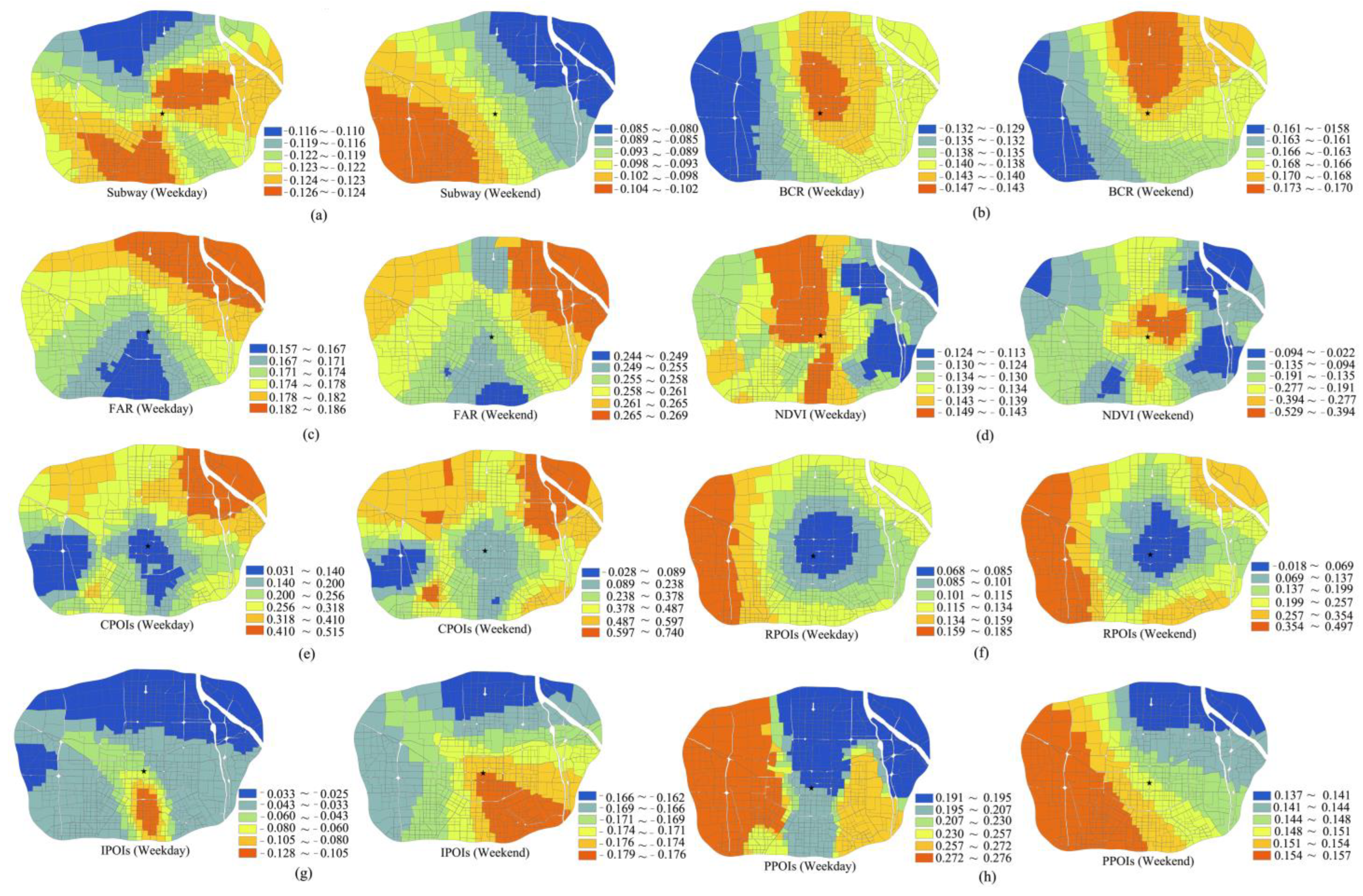
The spatial distribution of the coefficients for each significant built environment variable was determined (Figure 5). We represented the influencing intensity of the corresponding built environment variable of the street block according to the Jenks natural breaks method. Obviously, the spatial heterogeneous influence could be detected using the MGWR model, and some spatial differences could also be distinguished between workdays and weekends from the visualization.
For subways with a negative effect on population distribution, the farther the street block is from the nearest subway station, the lower the population density. The blocks with a large influencing intensity were mainly distributed in the eastern and southwestern parts, whereas small levels were distributed in the northern part of the city on weekdays. Notably a stagewise increase was found from the northeast to the southwest on weekends. As we know, these street blocks with large level of influencing intensity also have a high residential population and job-concentrated places, which may be more likely to be affected by traffic accessibility. The BCR also has a negative influence on population distribution, and the strength of the influence shows a similar spatial distribution between weekdays and weekends. The large influence is concentrated in the northern part of the urban center, which indicates that these street blocks with large building coverage may not have a high population density because the spatial distribution of the population in Xi’an is high in the south and low in the north. The western part of the city has been developing in recent years, and the population density is very low in these street blocks, which may result in insensitivity to the BCR. A similar spatial distribution was observed for FAR on both weekdays and weekends. The large level of influence intensity is mainly concentrated in the northeastern part of the city, which is oriented as an urban ecological and livable area with many green spaces. Therefore, street blocks with high FAR may have a large population density in these areas. The street blocks in the southern part of the city are well developed, have a high population density, and are less influenced by the FAR. From the spatial distribution of NDVI, street blocks with a small level of influence intensity are mainly located in urban areas with high green space (eastern part), which indicates that NDVI has less influence on the population density of these street blocks than in other areas.
In terms of POI-related variables, CPOI had a positive effect on the population density of street blocks, and there was a similar spatial distribution of coefficients between weekdays and weekends. While CPOI has high level of influence on population density in the ecological and livable area (northeast part), small influence happens around the urban center and its south, as well as the western part of the city. For ecological and livable areas, one characteristic is that some street blocks are covered by green space and have very low population density and few CPOI, whereas other street blocks include residential high-rise buildings around many CPOI. We conjecture that this characteristic may result in large regression coefficients for these street blocks because of local search in the MGWR model. These street blocks around the urban center and the southern part of the city include a large number of CPOI and simultaneously have a large population density; the influencing intensity of CPOI in these street blocks is relatively low.
The influence of the RPOI increased from the urban center to the periphery on both weekdays and weekends. The largest level of influence occurs in the western street blocks of cities, which are developing areas, through the building of residential communities and industrial parks. Regarding the spatial distribution of the influence of IPOI, some differences exist between weekdays and weekends. The IPOI had a positive influence on population density on weekdays, and the strong correlation is concentrated on the street blocks of the urban south-central region, which include numerous companies and enterprises. For the northern urban area with few enterprises, the influencing intensity of the IPOI is smaller than that in the southern urban area. On weekends, the IPOI has a negative influence on the population density of street blocks, and the strong influence is dominant in the urban southeastern part, which is covered by many residential communities, indicating that the greater the IPOI in these blocks, the lower the population density on weekends. It is obvious that PPOI has a strong correlation with population density in the western part of the city on both weekdays and weekends, which promotes an increase in population when the number of PPOI increases. The low-level influence of the PPOI was mainly distributed in the northeastern part of the city.

5. Discussion

This study attempts to address the research question: how the built environment factors affect the urban population distribution and how the influence changes over space and time. Based on the fine-resolution population distribution data, we investigate the dynamic relationship between built environment and population distribution in a rapid development city Xi’an, China. Previous studies mainly put attention on the well-developed and highly dense cities (e.g., Beijing, Shanghai), whereas the empirical analysis of rapid developing cities is little. Therefore, it is meaningful to explore the interaction between population distribution and built environment in a rapidly developing urban context, which could give some guidance to urban planning and renewal.
The results show that some built environment factors are strongly associated with population distribution. These findings can be generalized from three perspectives. First, human distribution showed a strong spatial autocorrelation for all time periods during the day, and the spatial distribution on weekends was more intensive than that on weekdays. This spatially heterogeneous distribution is mainly attributed to the spatially inhomogeneous distribution of resources, facilities, and land-use functions. Secondly, a temporally varying influence of the built environment on population distribution was detected, indicating that a dynamic relationship exists between the built environment and population distribution. Third, the spatially varying effects of built environment factors on the population distribution were quantified using the MGWR model. In other words, transport conditions, land use, and building footprint factors have different influences on population density at different locations in the city.
Awareness of urban population distribution and its relationship with the built environment could contribute to urban planning, traffic, and disaster management. Currently, there is an accelerated renewal of urban functions in Xi’an. The findings could help urban planners to estimate dynamic population distribution in advance for renewed places (e.g., urban village renovation from residential to commercial districts). In addition, spatially heterogeneous influence of the built environment indicates that the same built environment factor would generate a different influence on population distribution, which gives us a reference for the targeted location of some facilities for different places. For example, commercial facilities should be added in the northeast of the city rather than in the downtown areas. Moreover, an understanding of dynamic population distribution provides some valuable information for urban emergency management, e.g., assessing the affected population when disaster happens. Therefore, the findings enhance our knowledge of the spatiotemporal distribution of the population and its dynamic relationship with the built environment. This could provide guidance for urban planning and emergency management.

6. Conclusions

Population distribution changes over space and time, leading to a dynamic spatiotemporal landscape in the city. Moreover, the population distribution exhibited high spatial autocorrelation. Using Xi’an, China as a case study, this work aimed to investigate the spatiotemporal heterogeneous relationship between the built environment and population distribution. This could enrich the current literature from two perspectives. On the one hand, the high penetration of social media location data is used as a proxy of population distribution to portray human spatiotemporal dynamics, which is closer to the real scene of the city than static survey data and gives us the opportunity to investigate population distribution at a fine spatiotemporal resolution. On the other hand, the temporally and spatially varying influence of the built environment on population distribution was examined to compensate for traditional global relationships that neither consider temporal dynamic characteristics of population distribution nor spatial nonstationary relationships between the built environment and population distribution. Therefore, the empirical findings provide insights into the spatiotemporal heterogeneous mechanisms of urban population distribution.
However, this study has some limitations that should be addressed in future research. First, although social media location data have high permeability, they are not equivalent to real population distribution; thus, it is necessary to syndicate multisource data (e.g., mobile phone data and check-in data) to model the real population distribution. Second, only linear models were considered to quantify the relationship between built environment factors and population distribution, and some machine learning methods should be encouraged to check whether a nonlinear relationship exists between the built environment and population, which further provides a prediction of population distribution based on the built environment.

Author Contributions

Conceptualization, X.Y. and W.T.; methodology, X.Y., C.S. and Z.Z.; writing—original draft preparation, X.Y. and L.L.; writing—review and editing, supervision, X.Y. and W.T. All authors have read and agreed to the published version of the manuscript.

Funding

This research was funded by National Natural Science Foundation of China (NO. 42271468; 42201500), Open Fund of Key Laboratory of Urban Land Resources Monitoring and Simulation, Ministry of Natural Resources (NO. KF2022-07-005); Open Research Fund by Guangdong Key Laboratory of Urban Informatics (SZU51029202007) the Fundamental Research Funds for the Central Universities (GK202201008); Open funding of Key Lab of Spatial Data Mining & Information Sharing of Ministry of Education (2022LSDMIS03); Shenzhen Science and Technology Program (JCYJ20220818100200001).

Data Availability Statement

The data used in this study are available by contact with the first author.

Conflicts of Interest

The authors declare no conflict of interest.

References

  1. Yin, L.; Chen, J.; Zhang, H.; Yang, Z.; Wan, Q.; Ning, L.; Hu, J.; Yu, Q. Improving emergency evacuation planning with mobile phone location data. Environ. Plan. B Urban Anal. City Sci. 2020, 47, 964–980. [Google Scholar] [CrossRef]
  2. Hossain, M.K.; Meng, Q. A fine-scale spatial analytics of the assessment and mapping of buildings and population at different risk levels of urban flood. Land Use Policy 2020, 99, 104829. [Google Scholar] [CrossRef]
  3. Kandt, J.; Batty, M. Smart cities, big data and urban policy: Towards urban analytics for the long run. Cities 2021, 109, 102992. [Google Scholar] [CrossRef]
  4. Haraguchi, M.; Nishino, A.; Kodaka, A.; Allaire, M.; Lall, U.; Kuei-Hsien, L.; Onda, K.; Tsubouchi, K.; Kohtake, N. Human mobility data and analysis for urban resilience: A systematic review. Environ. Plan. B Urban Anal. City Sci. 2022, 49, 1507–1535. [Google Scholar] [CrossRef]
  5. Liu, Y.; Liu, X.; Gao, S.; Gong, L.; Kang, C.; Zhi, Y.; Chi, G.; Shi, L. Social sensing: A new approach to understanding our socioeconomic environments. Ann. Assoc. Am. Geogr. 2015, 105, 512–530. [Google Scholar] [CrossRef]
  6. Shaw, S.-L.; Tsou, M.-H.; Ye, X. Editorial: Human dynamics in the mobile and big data era. Int. J. Geogr. Inf. Sci. 2016, 30, 1687–1693. [Google Scholar] [CrossRef]
  7. Huang, B.; Wang, J. Big spatial data for urban and environmental sustainability. Geo. Spat. Inf. Sci. 2020, 23, 125–140. [Google Scholar] [CrossRef]
  8. Huang, H.; Yao, X.A.; Krisp, J.M.; Jiang, B. Analytics of location-based big data for smart cities: Opportunities, challenges, and future directions. Comput. Environ. Urban Syst. 2021, 90, 101712. [Google Scholar] [CrossRef]
  9. Deville, P.; Linard, C.; Martin, S.; Gilbert, M.; Stevens, F.R.; Gaughan, A.E.; Blondel, V.D.; Tatem, A.J. Dynamic population mapping using mobile phone data. Proc. Natl. Acad. Sci. USA 2014, 111, 15888–15893. [Google Scholar] [CrossRef]
  10. Ye, T.; Zhao, N.; Yang, X.; Ouyang, Z.; Liu, X.; Chen, Q.; Hu, K.; Yue, W.; Qi, J.; Li, Z.; et al. Improved population mapping for China using remotely sensed and points-of-interest data within a random forests model. Sci. Total Environ. 2019, 658, 936–946. [Google Scholar] [CrossRef]
  11. Shang, S.; Du, S.; Du, S.; Zhu, S. Estimating building-scale population using multi-source spatial data. Cities 2021, 111, 103002. [Google Scholar] [CrossRef]
  12. Rubinyi, S.; Blankespoor, B.; Hall, J.W. The utility of built environment geospatial data for high-resolution dasymetric global population modeling. Comput. Environ. Urban Syst. 2021, 86, 101594. [Google Scholar] [CrossRef]
  13. Chen, L.; Zhao, L.; Xiao, Y.; Lu, Y. Investigating the spatiotemporal pattern between the built environment and urban vibrancy using big data in Shenzhen, China. Comput. Environ. Urban Syst. 2022, 95, 101827. [Google Scholar] [CrossRef]
  14. Li, X.; Li, Y.; Jia, T.; Zhou, L.; Hijazi, I.H. The six dimensions of built environment on urban vitality: Fusion evidence from multi-source data. Cities 2022, 121, 103482. [Google Scholar] [CrossRef]
  15. Wang, X.; Zhang, Y.; Yu, D.; Qi, J.; Li, S. Investigating the spatiotemporal pattern of urban vibrancy and its determinants: Spatial big data analyses in Beijing, China. Land Use Policy 2022, 119, 106162. [Google Scholar] [CrossRef]
  16. Chen, J.; Pei, T.; Shaw, S.-L.; Lu, F.; Li, M.; Cheng, S.; Liu, X.; Zhang, H. Fine-grained prediction of urban population using mobile phone location data. Int. J. Geogr. Inf. Sci. 2018, 32, 1770–1786. [Google Scholar] [CrossRef]
  17. Liu, Z.; Ma, T.; Du, Y.; Pei, T.; Yi, J.; Peng, H. Mapping hourly dynamics of urban population using trajectories reconstructed from mobile phone records. Trans. GIS 2018, 22, 494–513. [Google Scholar] [CrossRef]
  18. Zhang, G.; Rui, X.; Poslad, S.; Song, X.; Fan, Y.; Wu, B. A method for the estimation of finely grained temporal spatial human population density distributions based on cell phone call detail records. Remote Sens. 2020, 12, 2572. [Google Scholar] [CrossRef]
  19. Li, M.; Gao, S.; Lu, F.; Liu, K.; Zhang, H.; Tu, W. Prediction of human activity intensity using the interactions in physical and social spaces through graph convolutional networks. Int. J. Geogr. Inf. Sci. 2021, 35, 2489–2516. [Google Scholar] [CrossRef]
  20. Bergroth, C.; Järv, O.; Tenkanen, H.; Manninen, M.; Toivonen, T. A 24-hour population distribution dataset based on mobile phone data from Helsinki Metropolitan Area, Finland. Sci. Data 2022, 9, 39. [Google Scholar] [CrossRef]
  21. Jacobs, J. The Death and Life of American Cities; Vintage Book Company: New York, NY, USA, 1961. [Google Scholar]
  22. Tu, W.; Zhu, T.; Xia, J.; Zhou, Y.; Lai, Y.; Jiang, J.; Li, Q. Portraying the spatial dynamics of urban vibrancy using multisource urban big data. Comput. Environ. Urban Syst. 2020, 80, 101428. [Google Scholar] [CrossRef]
  23. Chen, T.; Hui, E.C.M.; Wu, J.; Lang, W.; Li, X. Identifying urban spatial structure and urban vibrancy in highly dense cities using georeferenced social media data. Habitat Int. 2019, 89, 102005. [Google Scholar] [CrossRef]
  24. Huang, B.; Zhou, Y.; Li, Z.; Song, Y.; Cai, J.; Tu, W. Evaluating and characterizing urban vibrancy using spatial big data: Shanghai as a case study. Environ. Plan. B Urban Anal. City Sci. 2020, 47, 1543–1559. [Google Scholar] [CrossRef]
  25. Wu, C.; Ye, X.; Ren, F.; Du, Q. Check-in behaviour and spatio-temporal vibrancy: An exploratory analysis in Shenzhen, China. Cities 2018, 77, 104–116. [Google Scholar] [CrossRef]
  26. Jia, C.; Du, Y.; Wang, S.; Bai, T.; Fei, T. Measuring the vibrancy of urban neighborhoods using mobile phone data with an improved PageRank algorithm. Trans. GIS 2019, 23, 241–258. [Google Scholar] [CrossRef]
  27. Meng, Y.; Xing, H. Exploring the relationship between landscape characteristics and urban vibrancy: A case study using morphology and review data. Cities 2019, 95, 102389. [Google Scholar] [CrossRef]
  28. Kang, C.; Fan, D.; Jiao, H. Validating activity, time, and space diversity as essential components of urban vitality. Environ. Plan. B Urban Anal. City Sci. 2021, 48, 1180–1197. [Google Scholar] [CrossRef]
  29. Kim, Y.-L. Data-driven approach to characterize urban vitality: How spatiotemporal context dynamically defines Seoul’s nighttime. Int. J. Geogr. Inf. Sci. 2020, 34, 1235–1256. [Google Scholar] [CrossRef]
  30. Pan, Y.; Zeng, W.; Guan, Q.; Yao, Y.; Liang, X.; Yue, H.; Zhai, Y.; Wang, J. Spatiotemporal dynamics and the contributing factors of residential vacancy at a fine scale: A perspective from municipal water consumption. Cities 2020, 103, 102745. [Google Scholar] [CrossRef]
  31. Li, Z.; Jiao, L.; Zhang, B.; Xu, G.; Liu, J. Understanding the pattern and mechanism of spatial concentration of urban land use, population and economic activities: A case study in Wuhan, China. Geo. Spat. Inf. Sci. 2021, 24, 678–694. [Google Scholar] [CrossRef]
  32. Liu, X.; Huang, B.; Li, R.; Wang, J. Characterizing the complex influence of the urban built environment on the dynamic population distribution of Shenzhen, China, using geographically and temporally weighted regression. Environ. Plan. B Urban Anal. City Sci. 2021, 48, 1445–1462. [Google Scholar] [CrossRef]
  33. Li, M.; Tu, W.; Lu, F. Sensing the nighttime economy–housing imbalance from a mobile phone data perspective: A case study in shanghai. Remote Sens. 2022, 14, 2738. [Google Scholar] [CrossRef]
  34. Li, J.; Li, J.; Yuan, Y.; Li, G. Spatiotemporal distribution characteristics and mechanism analysis of urban population density: A case of Xi’an, Shaanxi, China. Cities 2019, 86, 62–70. [Google Scholar] [CrossRef]
  35. Yuan, J.; Zheng, Y.; Xie, X. Discovering regions of different functions in a city using human mobility and POIs. In Proceedings of the 18th ACM SIGKDD International Conference on Knowledge Discovery and Data Mining, Beijing, China, 12–16 August 2012; Association for Computing Machinery: Beijing, China, 2012; pp. 186–194. [Google Scholar] [CrossRef]
  36. Liu, X.; Long, Y. Automated identification and characterization of parcels with OpenStreetMap and points of interest. Environ. Plan. B Plan. Des. 2016, 43, 341–360. [Google Scholar] [CrossRef]
  37. Fotheringham, A.S.; Yang, W.; Kang, W. Multiscale geographically weighted regression (MGWR). Ann. Am. Assoc. Geogr. 2017, 107, 1247–1265. [Google Scholar] [CrossRef]
  38. Xia, C.; Yeh, A.; Zhang, A. Analyzing spatial relationships between urban land use intensity and urban vitality at street block level: A case study of five Chinese megacities. Lands Urban Plan. 2020, 193, 103669. [Google Scholar] [CrossRef]
  39. Yang, X.; Fang, Z.; Xu, Y.; Yin, L.; Li, J.; Lu, S. Spatial heterogeneity in spatial interaction of human movements—Insights from large-scale mobile positioning data. J. Transp. Geogr. 2019, 78, 29–40. [Google Scholar] [CrossRef]
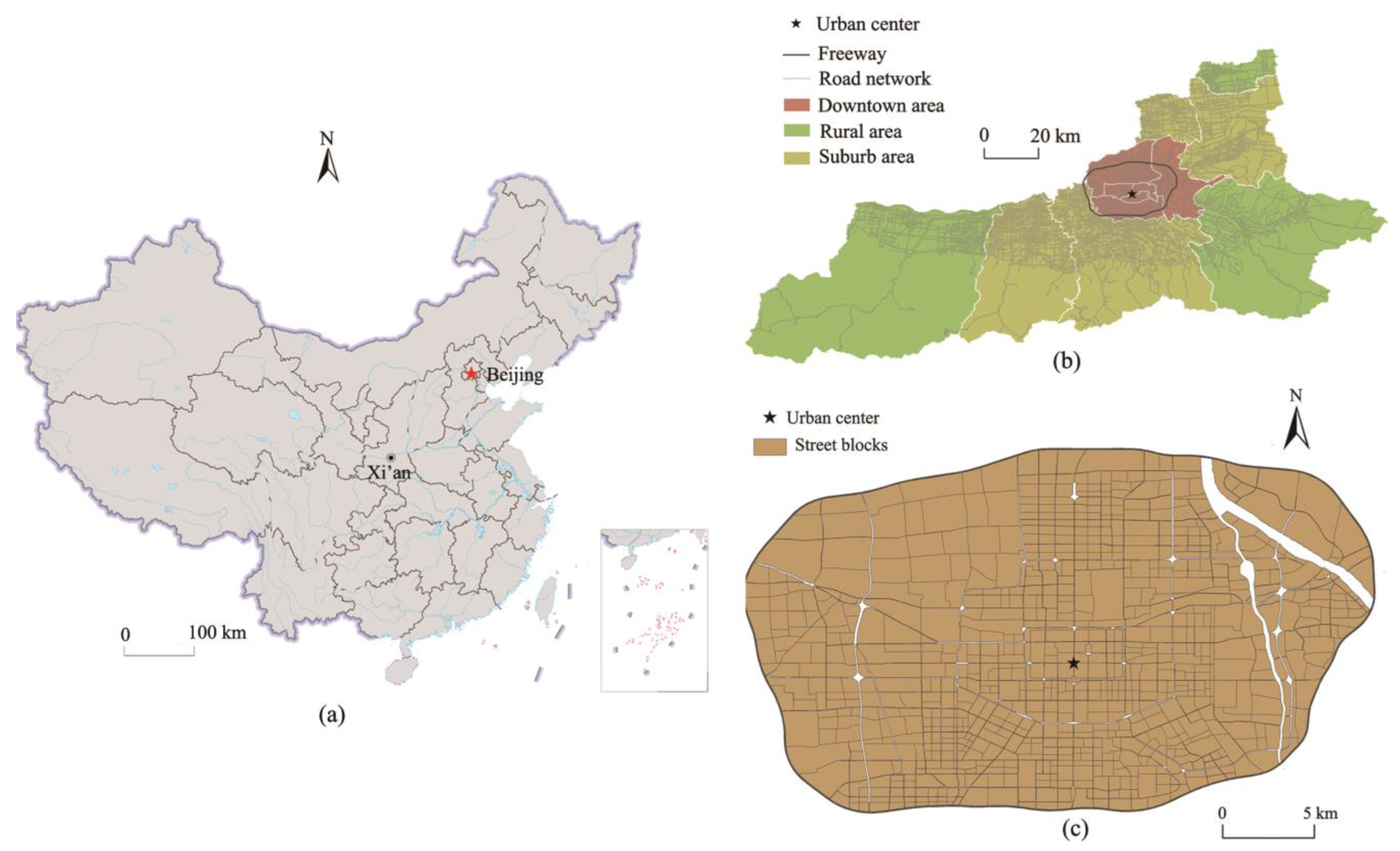
Figure 1. (a) The map of China, (b) The study area in Xi’an, (c) the street blocks divided by road lines.
Remotesensing 15 02257 g001
Figure 2. The kernel density of human distribution in a study area in the city of Xi’an northwestern China.
Remotesensing 15 02257 g002
Figure 3. (a) the Moran’s I index of human distribution and (b) the temporal change of goodness of fit for MGWR model.
Remotesensing 15 02257 g003
Figure 4. The dynamic change of coefficients for eight significant built environment variables over time in the study area in Xi’an in China, where (a) shows distance to the subway station (subway), (b) the building coverage rate (BCR), (c) the floor area rate (FAR), (d) the normalized difference vegetation index (NDVI), while (e) shows the commercial point of interest (CPOI), (f) the residential point of interest (RPOI), (g) the industrial point of interest (IPOI), and (h) to public point of interest (PPOI).
Remotesensing 15 02257 g004
Figure 5. Visual representation of the spatial varying coefficients of the multiscale geographically weighted regression (MGWR). Overall, the influencing coefficients exhibit a significant dynamic change, where (a) shows distance to the subway station (subway), (b) the building coverage rate (BCR), (c) the floor area rate (FAR), (d) the normalized difference vegetation index (NDVI), while (e) shows the commercial point of interest (CPOI), (f) the residential point of interest (RPOI), (g) the industrial point of interest (IPOI), and (h) to public point of interest (PPOI).
Remotesensing 15 02257 g005
Table 1. The independent variables used to describe the characteristics of the built environment during a study investigating the dynamic heterogeneous relationship between urban population distribution and the built environment in Xi’an, northwestern China.
NameDescription
TransportationRoad interaction ( R I i )The number of toad interaction within the street block.
Road density ( R D i )The density of road within the street block, calculated by R D i = L i A i , L i represents the length of road lines within the street block, and A i the area of the street block.
Bus stops density ( B u s D i )The ratio of total number of bus stops to the area of the street block.
Subway distance (SubwayD)The distance between center of street block to the nearest subway station.
LocationLocation ( L )The distance of each street block to the urban center.
Building footprintBuilding coverage ratio ( B C R i )The ratio of total building area to the area of street block B C R i = B i A i , B i denotes the total of building area.
Floor area ratio (FAR)The ratio of total floor area to the area of street block F A R i = F i A i , F i denotes the total of floor area within the street block.
GreenNDVI (NDVI)The average of NDVI within the street block.
Land usePOI density (POID)The ratio of total number of POI to area of street block.
Commercial POI density (CPOI)The ratio of total number of Commercial POI to area of street block.
Residential POI density (RPOI)The ratio of total number of Residential POI to area of street block.
Industrial POI density (IPOI)The ratio of total number of Industrial POI to area of street block.
Public POI density (PPOI)The ratio of total number of Public POI to area of street block.
POI mixed (POIM)The entropy of different type of POI within the street block. P o i E i = p i ln p i , p i represent the proportion of each type of POI.
Table 2. The regression result of the multiple linear regression model (MLR) used to estimate the global relationship between the built environment and population density in Xi’an northwestern China.
Independent VariablesWorkdayWeekend
Coefficientt-Statisticp-ValueCoefficientt-Statisticp-Value
Road interaction (RI)0.2157.2450.000 ***0.1716.3220.000 ***
Road density (RD)0.0110.3360.7370.0060.1830.855
Bus stops density (BusD)0.0150.6170.5380.0030.1320.895
Distance to subway station (Subway)−0.047−1.6600.047 *−0.082−3.2020.001 ***
Location (L)−0.033−0.8850.3770.0100.3060.760
Building coverage rate (BCR)−0.130−3.3360.001 ***−0.136−3.8180.000 ***
Floor area rate (FAR)0.2455.8960.000 ***0.3328.7770.000 ***
NDVI−0.102−3.5500.000 ***−0.123−4.7200.000 ***
Commercial POI (CPOI)0.1744.6710.000 ***0.2968.7300.000 ***
Residential POI (RPOI)0.0882.2940.022 **0.1363.8950.000 ***
Industrial POI (IPOI)0.0622.2720.023 **−0.123−4.9450.000 ***
Public POI (PPOI)0.2236.0860.000 ***0.1464.3700.000 ***
POI mixture (POIM)0.0170.5530.5810.0321.1290.259
AIC1835.4021729.07
R20.5280.609
Adjusted R20.5210.603
* significant level = 0.05, ** significant level = 0.01, *** significant level = 0.001.
Table 3. The summary statistics of regression of MGWR on weekday.
Independent VariableMinimumMeanMedianMaximumStd
Subway−0.125−0.122−0.125−0.1100.002
BCR−0.147−0.138−0.126−0.1290.004
FAR0.1570.1740.1650.1860.006
NDVI−0.149−0.135−0.132−0.1130.008
CPOI0.0310.2530.2550.5150.104
RPOI0.0680.1150.1220.1850.027
IPOI−0.128−0.042−0.048−0.0250.02
PPOI0.1910.2300.2230.2760.037
AIC1688.848
R20.648
Adjusted R20.610
Table 4. The summary statistics of regression of MGWR on weekend.
Independent VariableMinimumMeanMedianMaximumStd
Subway−0.104−0.093−0.093−0.0800.007
BCR−0.173−0.166−0.159−0.1580.003
FAR0.2440.2580.2520.2690.005
NDVI−0.529−0.182−0.190−0.0220.098
CPOI−0.0280.3860.3550.7400.174
RPOI−0.0180.2160.2090.4970.119
IPOI−0.179−0.171−0.172−0.1620.004
PPOI0.1370.1490.1500.1570.006
AIC1496.809
R20.748
Adjusted R20.720
Disclaimer/Publisher’s Note: The statements, opinions and data contained in all publications are solely those of the individual author(s) and contributor(s) and not of MDPI and/or the editor(s). MDPI and/or the editor(s) disclaim responsibility for any injury to people or property resulting from any ideas, methods, instructions or products referred to in the content.