Article

A Hybrid Framework for Simulating Actual Evapotranspiration in Data-Deficient Areas: A Case Study of the Inner Mongolia Section of the Yellow River Basin

1
State Key Laboratory of Earth Surface Processes and Resource Ecology, Beijing Normal University, Beijing 100875, China
2
Center for Geodata and Analysis, Faculty of Geographical Science, Beijing Normal University, Beijing 100875, China
*
Author to whom correspondence should be addressed.
These authors contributed equally to this work.
Remote Sens. 2023, 15(9), 2234; https://doi.org/10.3390/rs15092234
Submission received: 16 March 2023 / Revised: 4 April 2023 / Accepted: 19 April 2023 / Published: 23 April 2023
(This article belongs to the Section Remote Sensing in Geology, Geomorphology and Hydrology)

Abstract

:
Evapotranspiration (ET) plays an important role in transferring water and converting energy in the land–atmosphere system. Accurately estimating ET is crucial for understanding global climate change, ecological environmental problems, the water cycle, and hydrological processes. Machine learning (ML) algorithms have been considered as a promising method for estimating ET in recent years. However, due to the limitations associated with the spatial–temporal resolution of the flux tower data commonly used as the target set in ML algorithms, the ability of ML to discover the inherent laws within the data is reduced. In this study, a hybrid framework was established to simulate ET in data-deficient areas. ET simulation results of a coupled model comprising the Budyko function and complementary principle (BC2021) were used as the target set of the random forest model, instead of using the flux station observation data. By combining meteorological and hydrological data, the monthly ET of the Inner Mongolia section of the Yellow River Basin (IMSYRB) was simulated from 1982 to 2020, and good results were obtained (R2 = 0.94, MAE = 3.82 mm/mon, RMSE = 5.07 mm/mon). Furthermore, the temporal and spatial variations in ET and the influencing factors were analysed. In the past 40 years, annual ET in the IMSYRB ranged between 241.38 mm and 326.37 mm, showing a fluctuating growth trend (slope = 0.80 mm/yr), and the summer ET accounted for the highest proportion in the year. Spatially, ET in the IMSYRB showed a regular distribution of high ET in the eastern region and low ET in the western area. The high ET value areas gradually expanded from east to west over time, and the area increased continuously, with the largest increase observed in the 1980s. Temperature, precipitation, and normalized difference vegetation index (NDVI) were found to be the most important factors affecting ET in the region and play a positive role in promoting ET changes. These results provide an excellent example of long-term and large-scale accurate ET simulations in an area with sparse flux stations.

1. Introduction

Actual evapotranspiration (ET) refers to the total water vapor flux from vegetation and the ground to the atmosphere, including evaporation and transpiration [1,2]. Evaporation is the process by which water in soils, water bodies, and plant surfaces changes from a liquid or solid to a gaseous state, while the transpiration process occurs in the inter-vegetation system, by which water in plant cells diffuses to the outside world in the form of vapor through stomata or cuticles [3,4]. From the global land surface average, nearly 60% of global precipitation eventually evaporates into the atmosphere through different terrestrial ecosystems, accompanied by more than half of the net solar radiation consumption [5,6]. ET is not only the key factor maintaining the global land–air water balance, but also the main component of the energy balance, which plays a vital role in the hydrothermal cycle. In addition, as an important factor promoting atmospheric circulation, ET is also sensitive to climate change [7]. Therefore, it is critical to accurately estimate ET and reveal its spatiotemporal differentiation law for exploring the evolution and interaction mechanisms of water cycle components, as major climate change and increasing human activities continue to seriously impact the global natural ecosystem [8,9]. However, the lack of basic observation data and the limitation of the spatiotemporal resolution of remote sensing data make it difficult to accurately obtain long-term and large-scale surface ET.
Two main types of methods, actual measurement methods and simulation methods, have been developed for ET acquisition [10]. First, actual measurement methods take advantage of high precision and good time continuity but require high cost and are associated with site distributions [11]. Among such methods, the eddy covariance (EC) technique is generally considered the most accurate method for measuring ET [12], and many studies have used ET measurements obtained at flux stations as a basis to evaluate the reliability of other models [13]. The second way to obtain ET is through simulations, including remote sensing estimations, model simulations, and assimilations [14]. Such models are based on specific physical mechanisms with good spatial continuity and wide coverage. However, these models often have complex structures and require too many input parameters, inducing inevitable errors in the simulation results [15] and showing differential expressions among different regions and over different times. Overall, accurate ET estimations are still very difficult to achieve [16].
To provide reliable technical support for ET simulations and predictions, in recent years, the hydrological community has prepared to make full use of machine learning’s ability to mine massive amounts of data [17]. Machine learning (ML) models use specific algorithms to establish the nonlinear relationships between characteristics and target variables to achieve accurate predictions [18]. Therefore, their application effect is inevitably affected by the accuracy and scale of the input data [19]. Many scholars have used EC data as the target set to train ML models [20,21]. However, due to the sparse distribution of flux towers and the limited observation times, it is difficult to meet the ET simulation requirements at any spatiotemporal scale. Moreover, the quantity and quality of EC data also limit the prediction effects of ML models to a certain extent [22]. Therefore, it is necessary to find alternative ET data as the target sets to meet the needs of large-scale and long-term accurate ET simulations using ML models.
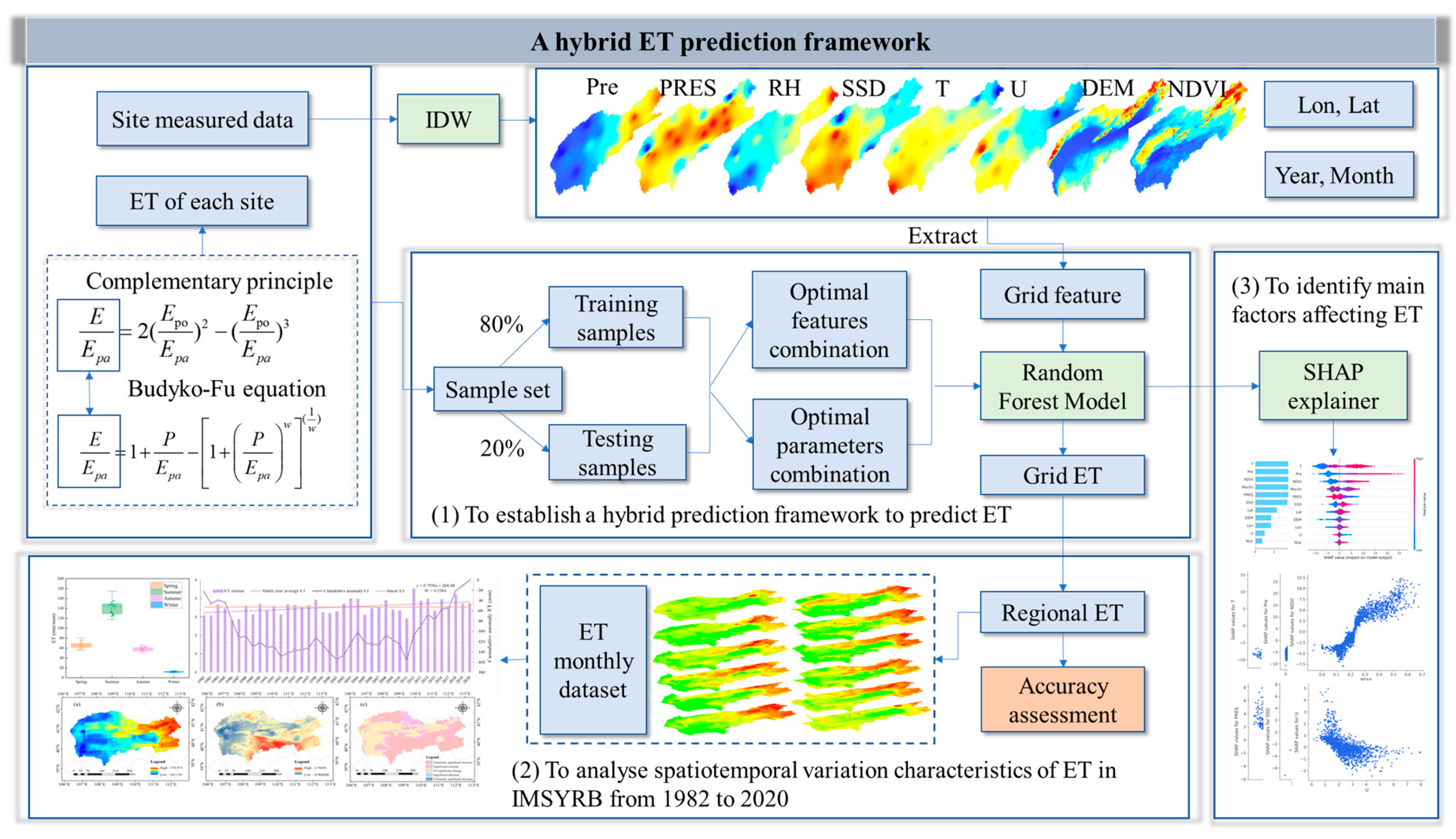
In view of the above deficiencies and requirements, we have established a new hybrid ET prediction framework to provide a good reference for ET estimation in areas with sparse flux towers. In this framework, we first use coupled model (BC2021) simulation results as the target set to establish a random forest model. The BC2021 model applied herein requires only basic meteorological data and can estimate site-scale ET at different time scales in areas lacking measured data [23], which provides the possibility for us to realize long-term ET simulations in data-deficient areas. Therefore, based on the ET prediction framework, this study takes the Inner Mongolia section of the Yellow River Basin (IMSYRB) as an example to carry out the following main objectives: (1) to establish a hybrid prediction framework to achieve regional ET simulation in the IMSYRB from 1982 to 2020; (2) to analyse the spatiotemporal variation characteristics of ET in the area; and (3) to identify the main factors affecting ET variations.

2. Materials and Methods

2.1. Study Area

The Yellow River enters Inner Mongolia from Shizuishan in Ningxia, flows through multiple administrative regions including Wuhai, Bayannur, Ordos, Baotou, and Hohhot, and finally exits from the Junge Banner. The total length of the Yellow River Basin in Inner Mongolia is 843 km, with an area of approximately 96,400 km2. This area belongs to the middle and upper reaches of the Yellow River Basin, accounting for approximately 20.6% of the total area of the Yellow River Basin. The IMSYRB is high in elevation in the middle region and low in the northern and southern areas, with an elevation range of 941 m to 2349 m (Figure 1). The annual average temperature of the region ranges from 4 °C to 8 °C, and the annual average precipitation ranges from 237 mm to 464 mm. The IMSYRB has sufficient light and strong solar radiation, and the annual sunshine hours are basically distributed in the range of 2000 h to 4300 h.
In recent years, due to global climate change and rapid regional economic development, the ecosystem of the IMSYRB has been continuously degraded, and the hydrological function has continued to decline. At the same time, artificial ecological restoration has led to the continuous growth of vegetation indices, and the ecological environment and water resources of the basin are facing severe situations; these conditions have formed a bottleneck, restricting regional ecological protection and high-quality development [24]. However, there are only 23 meteorological stations and one flux station in this area, because of the geographical location of the study area, alongside other reasons. The observational coverage of meteorological and hydrological elements is thus insufficient, and the observation stations are sparse and spatially discontinuous. Therefore, the IMSYRB is defined as a data-deficient area.

2.2. Data Collection and Processing

2.2.1. Basin Basic Data

The Digital Elevation Model (DEM) data used in this study were obtained by clipping a 1-km digital elevation map of China [25] provided by the National Qinghai-Tibet Plateau Data Center (https://data.tpdc.ac.cn, accessed on 30 May 2022). The meteorological data measured at 23 meteorological stations in the region were collected from the daily dataset (V3.0) of China’s surface climate data provided by the China Meteorological Data Network (http://data.cma.cn, accessed on 30 May 2022) The dataset included daily precipitation (Pre), temperature (T), wind speed (U), sunshine duration (SSD), air pressure (PRES) and other data, and the data accuracy is close to 100%. All meteorological data were checked using climate thresholds and for data consistency before use, and missing values were supplemented by linear interpolation. In addition, the spatial distributions of these meteorological data were obtained by the inverse distance weight method (IDW). The monthly normalized difference vegetation index (NDVI) dataset was downloaded from the Earth Science System Science Data Center (http://www.geodata.cn, accessed on 30 May 2022). The specific information of these data is shown in Table 1. Before use, the above data were unified to a 5-km resolution and to the WGS1984 coordinate system through the ArcGIS10.2 platform.

2.2.2. Evapotranspiration Dataset

In this study, the data measured at the Hobq Desert 05 (KBQ05) flux station and the open Global Land Evaporation Amsterdam Model (GLEAM), as well as the Global Land Data Assimilation System (GLDAS) datasets, were collected to verify the ET accuracy. The KBQ05 station is located in the middle of the study area (40°32′N, 108°41′E), and the main vegetation type near this station is artificial poplar forests. The measured data were obtained from the ChinaFLUX network (http://www.chinaflux.org/, accessed on 30 May 2022). This dataset included air temperature (T, °C), latent heat flux (LE, W·m−2), and sensible heat flux (Hs, W·m−2) data recorded every half hour from January 2006 to August 2009, with its energy closure rate reaching 80%. The GLEAM and GLDAS datasets can be obtained free of charge from the official GLEAM website (https://www.gleam.eu/, accessed on 30 May 2022) and the Earthdata website (https://search.earthdata.nasa.gov, accessed on 30 May 2022), respectively. The GLEAM product has been revised regularly since its release. In this study, we used the GLEAM v3.6a ET product for analysis. For the GLDAS dataset, the monthly ET data from 1982 to 1999 belong to the GLDAS NOAH 2.0 version, and the data from 2000 to 2020 belong to the NOAH 2.1 version. Similarly, a uniform spatial resolution of 5 km × 5 km was required before use.

2.3. Methods

Figure 2 summarizes the methods involved in this study, which consists of three main components: ET prediction framework establishment methods, spatiotemporal analysis methods, and impact factor identification methods. These are explained in detail below. The abbreviations mentioned in the article are detailed in Nomenclature.

2.3.1. A Hybrid ET Simulation Framework

In this study, the simulation results of the BC2021 model combining the Budyko equation and the complementary principle were used in the target set of the random forest model. The following text introduces the basic principles of the BC2021 and random forest models.
(1)
BC2021 Model
The complementary principle is a simple method applied to estimate ET using only basic meteorological data [26]. The initial complementary principle is completely symmetrical. It holds that when the supply of land surface water decreases, the increase in potential evapotranspiration is equal to the decrease in ET [27].
E p a E p o = E p o E
Later, scholars found that an increase in potential evapotranspiration is not exactly equal to the decrease in ET; that is, there is an asymmetric relationship between these variables [28]. In 2015, Brutsaert [29] expressed the relationship between EpaEpo and EpoE as a cubic polynomial based on the following asymmetric relationship:
E = ( E p o E p a ) 2 ( 2 E p a E p o )
or:
E E p a = 2 ( E p o E p a ) 2 ( E p o E p a ) 3
where E is the actual evapotranspiration; Epa is the demand for atmospheric evaporation; and Epo is the amount of evaporation when the external input energy is constant and the water supply is sufficient, also called wet surface evapotranspiration. Epa can be calculated using Penman’s simple empirical equation [30], and Epo can be expressed as the product of a constant αc = 1.26 [31] and the equilibrium evaporation term Ee (Ee = ∆Qne/(∆ + γ)). Many studies have used the parameter αc as a constant to estimate evapotranspiration. However, subsequent studies have shown that αc is a variable quantity [32], and its value depends on the size of the drought index (AI = Epa/P).
Initially, Budyko stated that water supply and energy supply were the limiting conditions of ET on annual and multiyear scales, namely, the Budyko hypothesis [33]. On this basis, the water–heat coupled energy balance equation for extreme wetness was established. Subsequently, considering the influence of the underlying surface of the basin, scholars proposed a series of Budyko correction equations, among which the following Fu equation is the most widely used [34]:
E E p a = 1 + P E p a [ 1 + ( P E p a ) w ] ( 1 w )
where ω is a parameter related to the underlying surface of the basin, with a value set to 2.41 in this study, and P is precipitation, measured in mm.
Zhang and Brutsaert eliminated the common terms in Equations (3) and (4) and used βcEe to represent Epo. Therefore, a coupling model (BC2021) of the complementary principle and the Budyko function can be obtained with the following simple expression:
x 3 2 x 2 + z = 0
where x = βcEe/Epa, y = E/Epa z = 1 + ( P / E p a ) [ 1 + ( P / E p a ) ω ] 1 / ω .
The solution of Equation (5) can be written as follows:
β c = Ω 1 [ 4 3 sin 1 ( 1 3 sin 1 ( 27 16 F ( Φ ) 1 ) ) + 2 3 ]
where Ω = Ee/Epa, Φ = P/Epa, F(Φ) = 1 + Φ − [1 + Φω]1/ω, and βc is a time-varying parameter that does not need to be calibrated. Simulated ET values at different time scales can be obtained by substituting βc into Equation (4). For more details about this model, please refer to [23].
(2)
Random Forest Algorithm
Random forest (RF) is an ensemble algorithm based on decision trees [35] that trains multiple classification and regression trees by randomly selecting sample points and a certain number of candidate attribute features in the original dataset. The results of multiple classification and regression trees are integrated to improve the prediction accuracy. The RF algorithm can handle high-dimensional data without requiring special preparation or feature selection. Compared to the ordinary regression tree method, the correlations between the multiple trees generated by different random subsets are low, so the method has the advantages of anti-noise and does not easily submit to overfitting. Because of its simple structure and high precision, the RF algorithm has been widely used in the field of earth science [36].
The specific steps of the regression algorithm based on the RF are as follows. In step 1, the sample set X is sampled based on the bootstrap method, generating t training sets randomly and further providing the corresponding decision trees; in step 2, m (m < M) is selected randomly from all M features as the feature set of the decision tree splitting; in step 3, all decision trees are generated without pruning; and in step 4, all trees are used to predict new sample points, and the mean predicted by each tree is taken as the final predicted value. The process of the RF model can be expressed as follows:
g ^ r f T ( x ) = 1 T t = 1 T T t ( x , θ t )
where Tt represents the prediction result of decision tree t, T is the number of decision trees, x is the input feature, and θt describes the terminal node values, segmentation variables, and other parameters in RF [37]. For a more detailed description of the RF, see Breiman (2001).

2.3.2. Explainable Machine Learning Methods

Traditional feature importance tells us the most important features but cannot illustrate how these important features affect the model prediction results. SHAP (Shapley additive explanations) is a game theory method proposed by Lundberg et al. [38] to explain the outputs of ML models, which can help us better understand the decision-making mechanisms of models. In this method, a linear additive model is constructed, the features are attributed, and the dimensionless SHAP value is used to reflect the feature influence on the model output. SHAP defines the predicted value as the sum of the SHAP values of each input feature as follows:
g ( X ) = φ 0 + i = 1 M φ i
where M is the number of input features, φi is the attribution value of each feature, and φ0 is a constant that explains the model, that is, the predicted mean of all training samples. The SHAP value is theoretically optimal, but its computational complexity is relatively high. Therefore, Lundberg et al. derived a tree ensemble algorithm, TreeSHAP, specifically for tree-based ensemble learning models [39]. The TreeSHAP algorithm uses the conditional expectation function to combine the interaction effects of features into the Shapley function and explains the model through the visualization of complex individual features. This method is superior to the traditional feature-attribution method [22].

2.3.3. Model Validation and Evaluation Methods

In this paper, the root mean square error (RMSE), mean absolute error (MAE), and determination coefficient (R2) were used to evaluate the accuracy of the above interpolation methods and of the ET simulation outputs:
R M S E = i = 1 n ( E T 0 i E T m i ) 2 n
M A E = 1 n i = 1 n | ( E T m i E T 0 i ) |
R 2 = 1 i = 1 n ( E T 0 i E T m i ) 2 i = 1 n ( E T 0 i E T ¯ 0 ) 2
where ET0 is the reference value of actual evapotranspiration; ETm is the model-simulated value;  E T 0 ¯  is the average reference value; i is the sample serial number; and n is the total number of samples. Higher R2, i.e., closer to 1, and lower RMSE/MAE, i.e., closer to 0, values indicate that the model better approximated the observed data. For example, for an ideal model, RMSE/MAE = 0 and R2 score = 1.

2.3.4. Analysis Methods of Temporal and Spatial Variations

Simple linear regression (SLR) is used to calculate the ET trend in this study. SLR is a parameter estimation method usually used to analyse the monotonic trends of a time series, especially for fitting the slopes of hydrometeorological variables over time [40]. The SLR equation is expressed as follows:
S l o p e = n × i = 1 n ( i × E T i ) i = 1 n i i = 1 n E T i n × i = 1 n i 2 ( i = 1 n i ) 2
where Slope is the slope of the linear fitting trend line, n is the total number of periods, and ETi is the actual evapotranspiration of period i. Slope > 0 indicates that ET showed an increasing trend during the period, and vice versa. The significance of the changes was calculated using t tests, and the ET change trends were divided into 5 levels according to the test results: extremely significant decrease (Slope < 0, p < 0.01), significant decrease (Slope < 0, 0.01 < p < 0.05), no significant change (p > 0.05), significant increase (Slope > 0, 0.01 < p < 0.05), and extremely significant increase (Slope > 0, p < 0.01).

3. Results

3.1. Model Validation and Parameter Selection

3.1.1. Verification of BC2021 Simulation Results

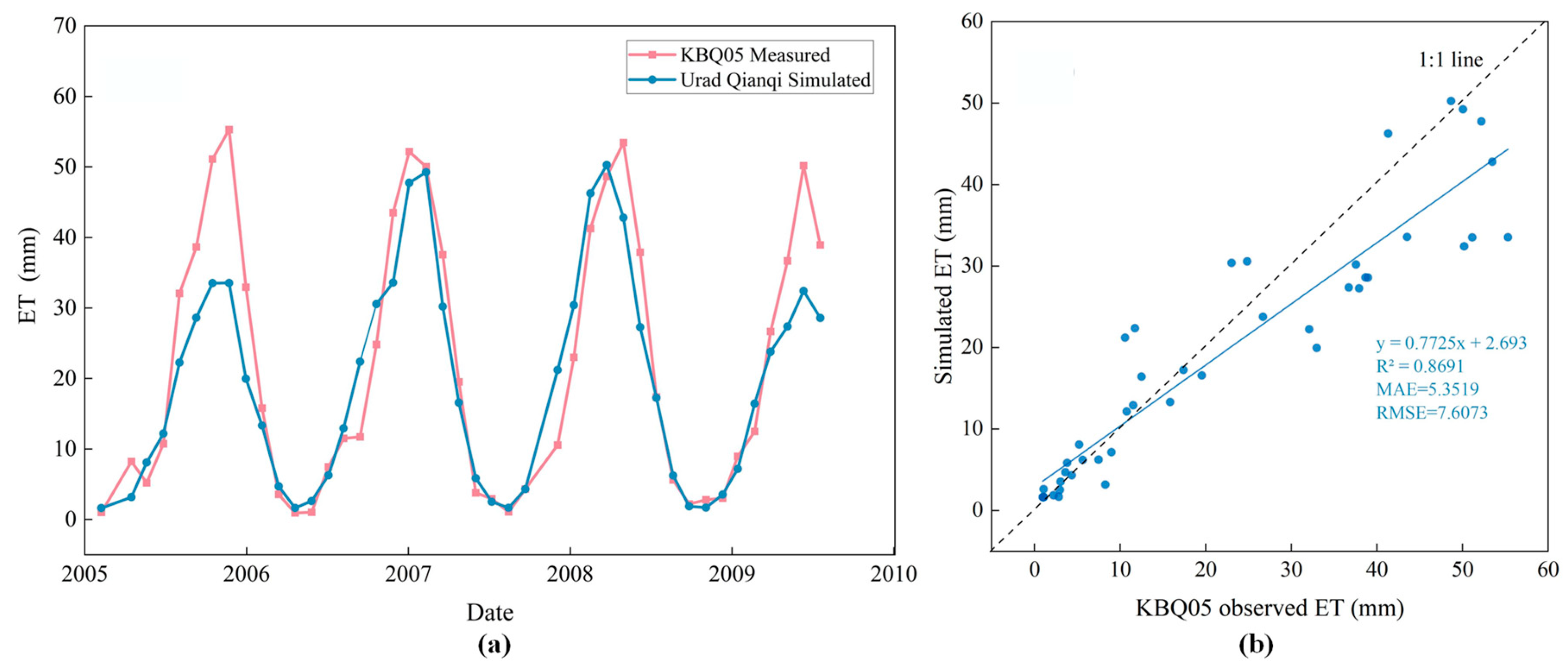
The monthly ET at the 23 station locations from 1982 to 2020 was calculated using BC2021 based on the daily meteorological data provided by 23 meteorological stations in the basin. To verify the model simulation accuracy and its applicability in the IMSYRB, we compared the ET data measured at the KBQ05 flux tower in the region with the simulated ET of the adjacent Urad Qianqi meteorological station. The results are shown in Figure 3.
Figure 3a shows the variations in the measured ET at the KBQ05 flux station and simulated ET at the Urad Qianqi weather station with time. These two variation trends show good consistency from January 2006 to August 2009, but the simulated values are obviously underestimated in the growing seasons of 2006 and 2009. Figure 3b shows the degree of fit between the simulated and measured values at the site scale. Because the two sites used for comparison are not located in exactly the same place, the meteorological and topographic conditions are different, so errors are inevitable when directly comparing the two series. In the case of inaccurate comparisons and limited measured data, a proportional relationship of 0.77 is still obtained between the simulated and measured values. The determination coefficient of the relationship is 0.87, and the MAE and RMSE values are 5.35 mm/mon and 7.60 mm/mon, respectively, indicating that the overall results of the model simulation seem to be satisfactory. The site-scale simulation accuracy even exceeds the accuracies of commonly used remote sensing and hydrological models. Therefore, we can conclude that the simulation results of the BC2021 model are reliable. Moreover, BC2021 has a good application effect in the IMSYRB, and its simulation results can be used as target values for establishing RF models.

3.1.2. Determination of RF Input Variables and Parameters

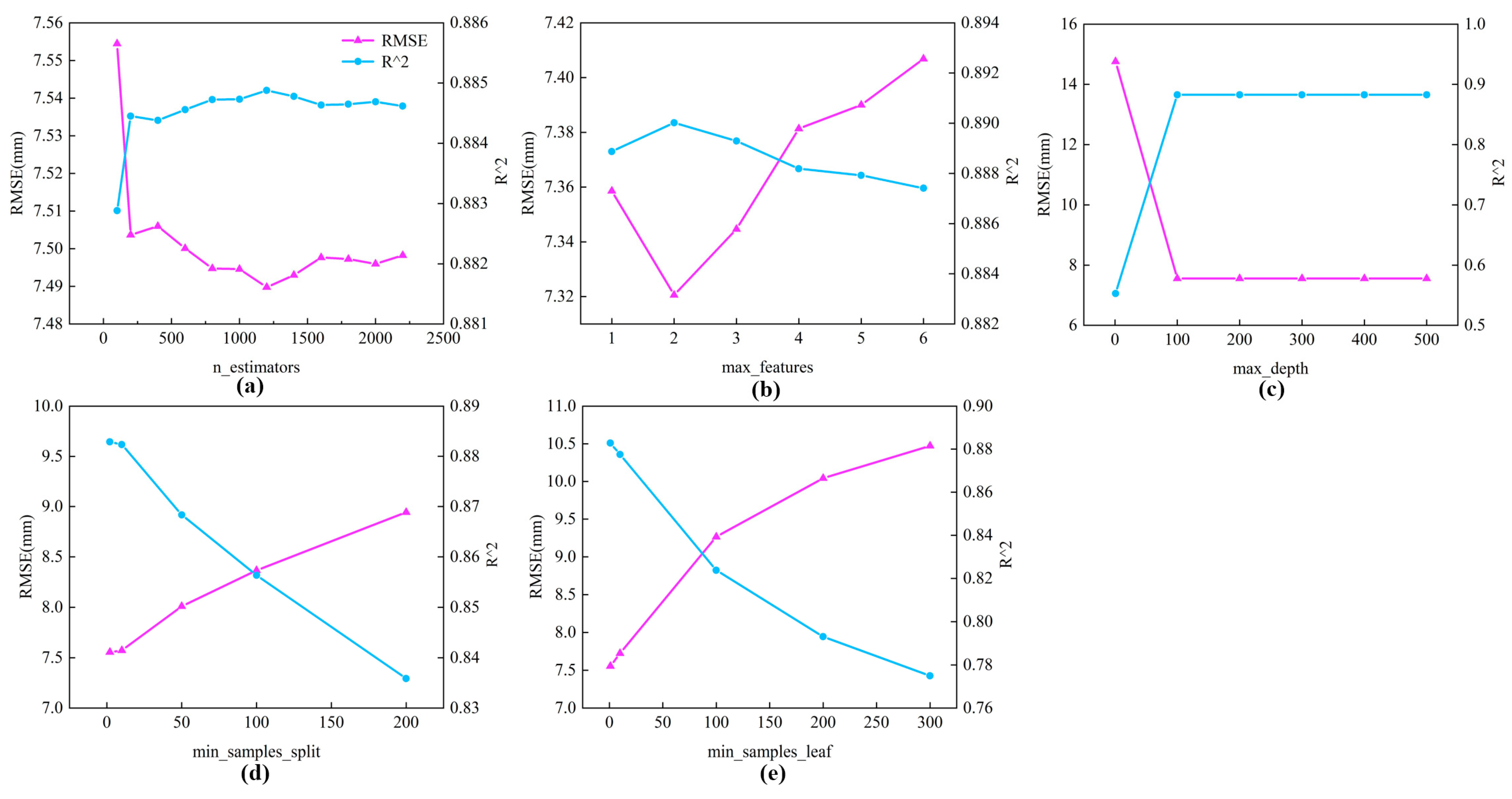
The RF simulation results depend mainly on five hyperparameters, including the tree number in the forest (n_estimators), the maximum depth of the trees (max_depth), the minimum sample number required to split the internal nodes (min_samples_split), the minimum sample number required on the leaf nodes (min_samples_leaf), and the number of features considered when finding the best split (max_features). Since the traditional method of using grid search to determine hyperparameters is too computationally expensive, we preliminarily evaluated the impact of each individual hyperparameter on the model to determine the parameter set. When applying the RF model, the input data were divided into 80% for the training set and 20% for the validation set. A 10-fold cross-validation method was used to assess the model performance driven by the corresponding parameters. RMSE and R2 were used as the evaluation indicators.
Figure 4 shows the effects of considering certain hyperparameters in the RF when other hyperparameters are defaulted. It can be seen that when max_depth exceeds 100, the increase in its value does not continuously improve the model prediction effect, so max_depth is defined as 100 without calibration; for min_samples_split and min_samples_leaf, the rise of their values has a significant negative impact on the improvement of the model prediction effect. Therefore, it is unnecessary to calibrate these two parameters, and the default values 2 and 1 are directly selected. For min_sample_split and min_sample_leaf, the increase in their values leads to the fluctuation of R2 and RMSE, so they need to be further calibrated to determine the parameter combination that makes the model achieve the best effect. Finally, the value of n_estimators and max_features are defined as 1600 and 2, respectively.
Theoretically, changes in ET are influenced by the water supply (precipitation and soil moisture), atmospheric evaporation demand (temperature, radiation, humidity, and wind speed), and vegetation physiological characteristics (LAI and NDVI) [8]. Therefore, precipitation (Pre), temperature (T), relative humidity (RH), wind speed (U), air pressure (PRES), sunshine duration (SSD), and NDVI are used as part of the input data combination in the RF model. In addition, to increase the data types and volume considered, allow the model to better discover the nonlinear relationships between variables and realize the prediction of monthly ET on the grid scale, the longitude (Lon), latitude (Lat), year (Year), month (Month), and DEM were also added to the model as the basic input features. Under this parameter combination, the R2 value between the simulation results and the KBQ05 observations was 0.89, and the MAE and RMSE values were 4.79 mm and 7.25 mm, respectively, indicating that the RF model established in this study has a certain reliability.

3.1.3. Verification of the Hybrid ET Prediction Framework Results

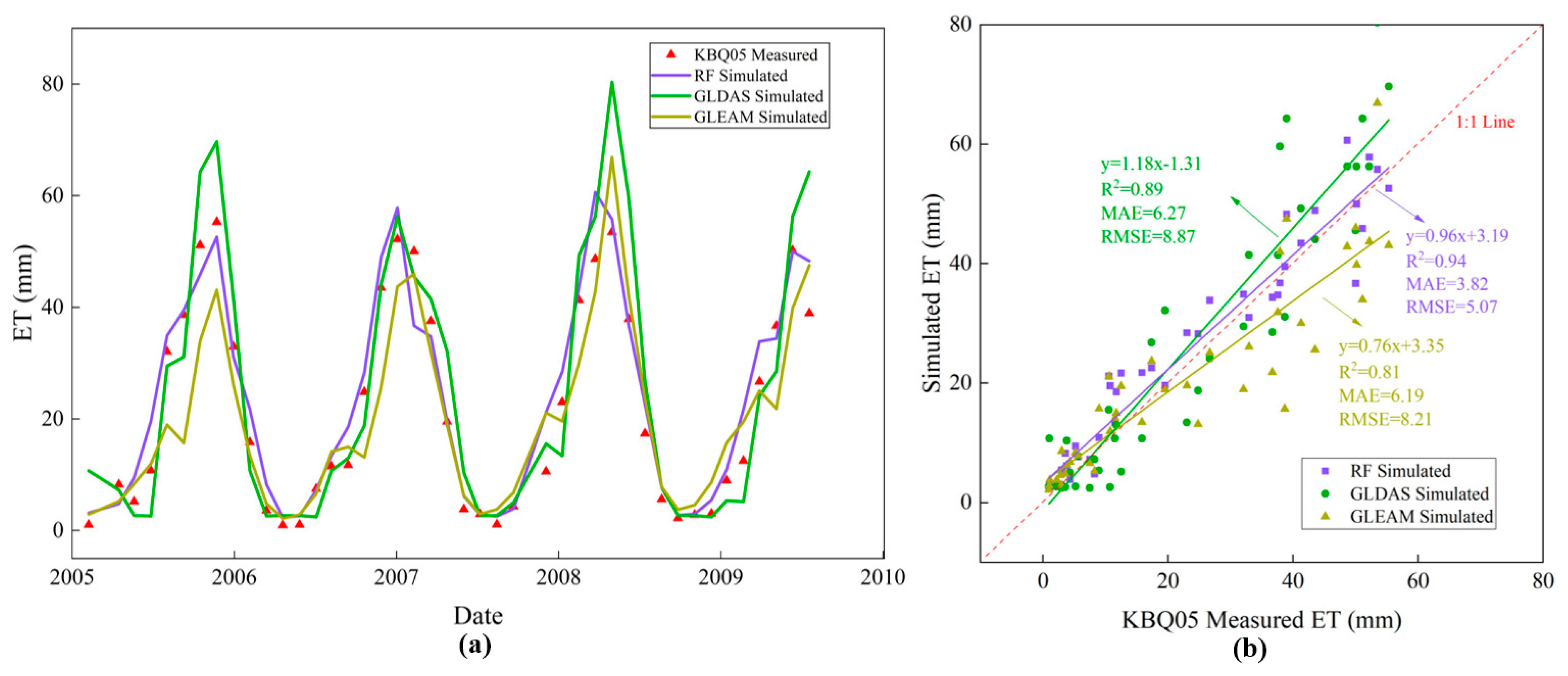
Section 3.1.1 proves the applicability of the site-scale BC2021 model in the study area. Therefore, the monthly ET values simulated at the 23 sites by the BC2021 model were taken as the target data, the 11 elements related to time, location, meteorology, hydrology, and topography selected in Section 3.1.2 were used as features to establish the RF model. Then, by inputting surface data of these features into the established model, the spatial distribution of ET in the IMSYRB from 1982 to 2020 was then output. The values simulated at the flux stations from January 2006 to August 2009 were extracted for comparison with the values measured at KBQ05 (Figure 5) to further verify the ET simulation results obtained with the combination of the BC2021 and RF models. At the same time, the values of the corresponding positions in the GLEAM and GLDAS datasets were also extracted to test the rationality of the thematic map produced in this study.
The RF simulation results have the best fitting effect with the measured values, and the peak prediction and temporal variation of ET are better than those of the GLEAM and GLDAS datasets (Figure 5). The GLDAS data generally overestimated ET, while the GLEAM data underestimated ET. The corresponding MAE and RMSE values are approximately 6 mm/mon and 8 mm/mon, respectively, exhibiting certain deviations from the actual values. In contrast, the multiple relationships between the RF simulation results and measured values is close to 1 (0.96). The R2 values are as high as 0.94, and the MAE and RMSE values are as low as 3.82 mm/mon and 5.07 mm/mon, respectively, indicating that RF shows a satisfactory prediction performance. Compared to the ET values of the adjacent Urad Qianqi station, R2 increased by 10.1%, and the MAE and RMSE values decreased by 2.9% and 33.3%, respectively.
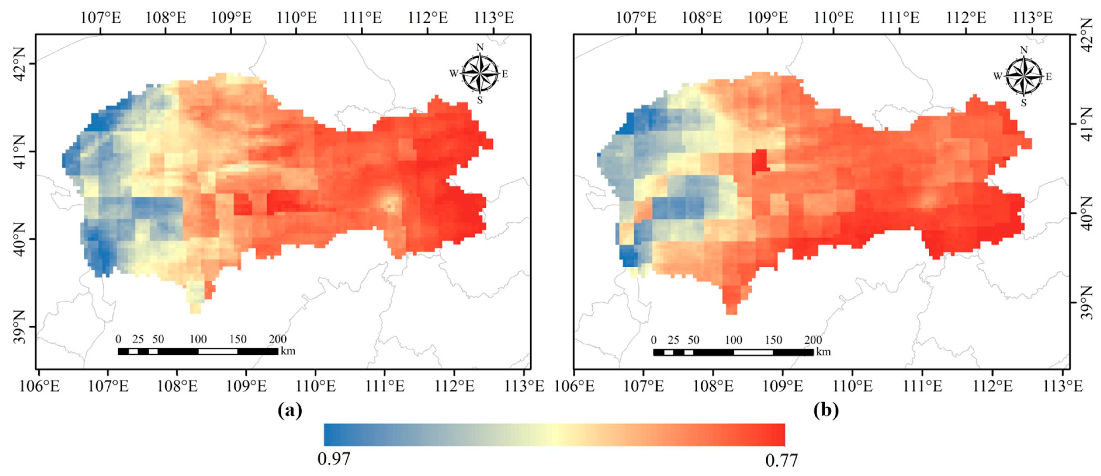
To further test the reliability of the RF model in predicting the spatial distribution of ET in the IMSYRB, a correlation analysis between the thematic map and the public dataset was conducted. Figure 6a shows the good correlation between the RF simulation results and the GLDAS dataset, with the minimum r value being 0.80 and the maximum r value reaching 0.96. In the spatial distribution of r, the correlation between the simulation results and the GLEAM data in the eastern part of the basin is stronger than that in the western part, and from east to west, r shows a decreasing trend. A similar spatial distribution pattern is shown in Figure 6b, with high values in the eastern region and low values in the western area. In terms of the values, the lowest r value is 0.77 and the highest is 0.97. These results show that although there are some errors, the spatial distribution of ET in the IMSYRB predicted by the RF model is credible and can be used to analyse the spatiotemporal variation in ET on long time scales.

3.2. Analysis of the Spatiotemporal Variation in ET in the IMSYRB

3.2.1. Temporal Variation Characteristics of ET in the IMSYRB

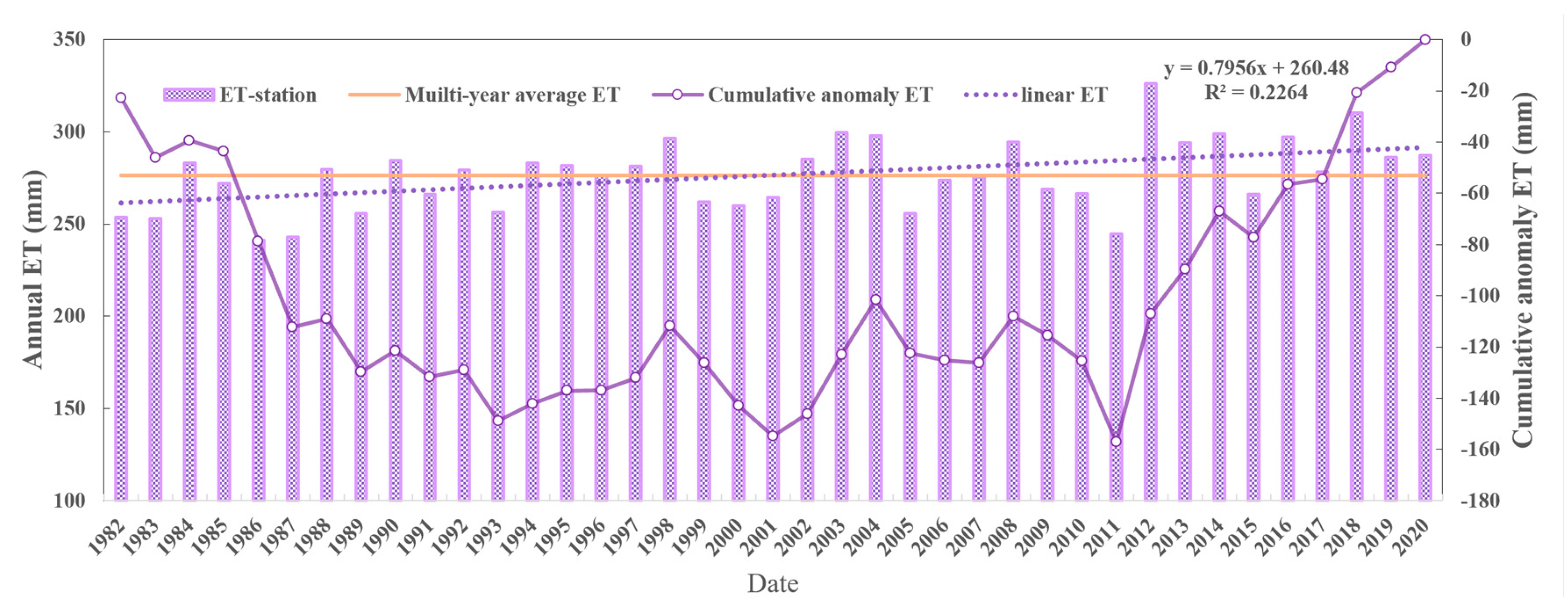
Based on the simulated monthly ET, the annual values were calculated, and then the changes in ET in the IMSYRB with time were analysed. Figure 7 shows the interannual variation map of ET in the IMSYRB. The average annual ET from 1982 to 2020 was 276.39 mm, and the ET changed in the range of 241.38 mm to 326.37 mm; the minimum value appeared in 1986, and the maximum value appeared in 2012. The regional ET showed a trend of fluctuating growth with time over the past 40 years, and the overall growth rate reached 0.80 mm/yr (R2 = 0.23). The cumulative anomaly curve of ET showed a ‘W’-type distribution law of decreasing–fluctuating–increasing, and no obvious change trend mutation point was identified.
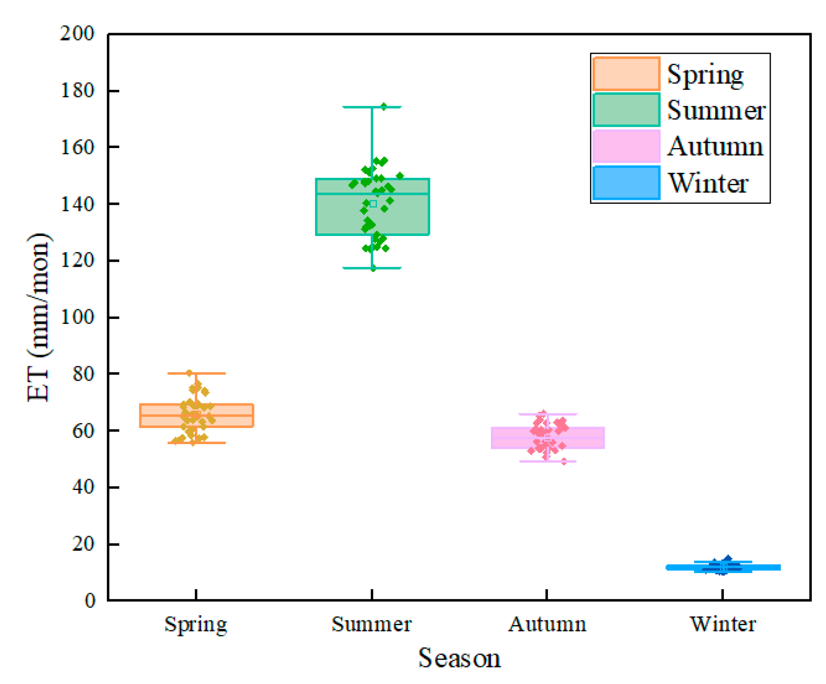
To study the annual variation in ET, the study period was categorized into the spring season spanning from March to May, summer from June to August, autumn from September to November, and winter from December of one year to February of the next year. The average ET in summer (140.54 mm) > spring (65.97 mm) > autumn (57.81 mm) > winter (12.08 mm), with these seasons accounting for 50.9%, 23.9%, 20.9%, and 4.4% of the whole year, respectively (Figure 8). The summertime ET fluctuations were the most obvious, and the interannual range reached 56.86 mm, followed by spring and autumn. The wintertime ET was basically stable, and the interannual range was only 4.53 mm.

3.2.2. Spatial Variation Characteristics in ET in the IMSYRB

The spatial distribution in ET in the IMSYRB is shown in Figure 9a. Affected by meteorological, hydrological, vegetation, and topographic factors, the average annual ET in the region from 1982 to 2020 showed obvious zonal characteristics, with high values in the eastern region and low values in the western region. The high-value areas were concentrated in Hohhot, Ulanqab, and Baotou, while the low-value areas were concentrated in Bayannur and Ordos. This spatial differentiation of ET is probably related to land cover. The land use types in the eastern part of the region mostly comprise cultivated lands and forestlands, and the vegetation coverage is dense. Abundant precipitation also promotes the transpiration of vegetation, resulting in large ET values. In the western region, unused lands and grasslands are the main land cover types. The sparse distribution of vegetation and the lack of precipitation in this area lead to the low ET levels. In addition, due to the influence of meteorological factors, the effect of altitude on the spatial distribution of regional ET is not obvious.
The slopes of the interannual variation in ET from 1982 to 2020 obtained from the SLR analysis were between −0.91 mm/yr and 2.74 mm/yr, indicating spatial differences in the ET trend within the IMSYRB. Combining Figure 9b,c and Table 2, it can be seen that over the past 40 years, (1) The spatial variation of ET showed an extremely significant increase, and the sum of these two increase types accounted for 64% of the total area. Throughout the region, the areas with extremely significant ET increases accounted for approximately 1/2 of the area, mostly distributed in Ordos in the southern part and the Hunhe River Basin, with significant green vegetation, in the eastern part. (2) The ET reduction area was distributed mainly in Bayannaoer, with low elevations and a low vegetation density, and in southern Baotou and northern Hohhot, and the reduction rate reached −0.91 mm/yr. The results of the T test show that the change trends in these ET reduction areas were not significant, and only less than 1% of the area showed significant characteristics.
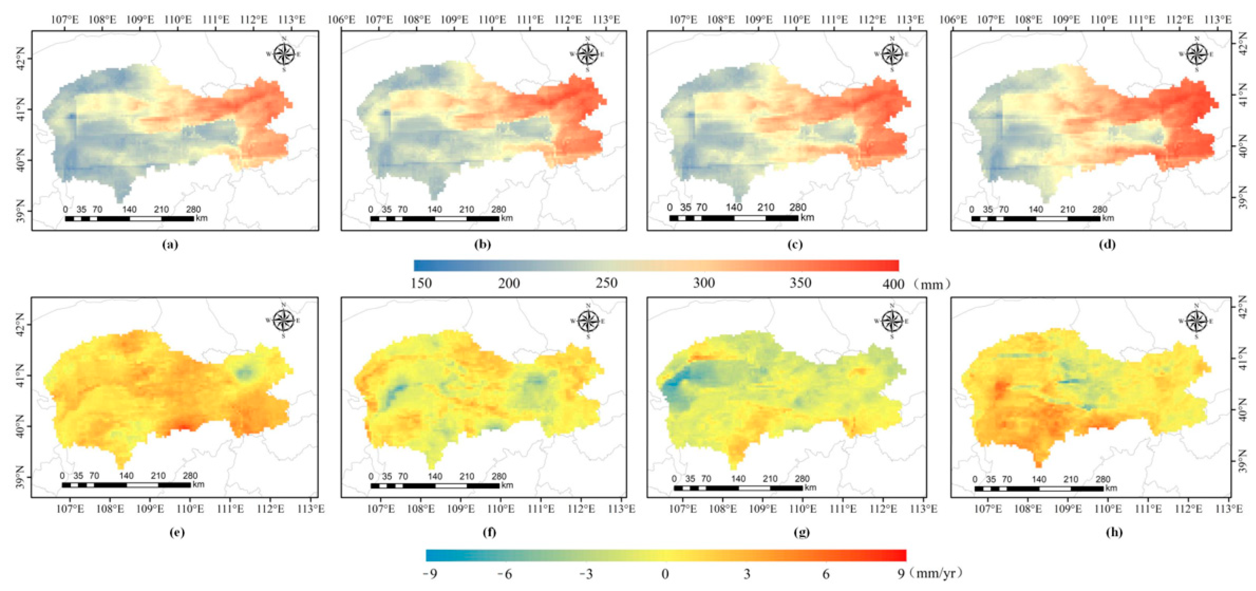
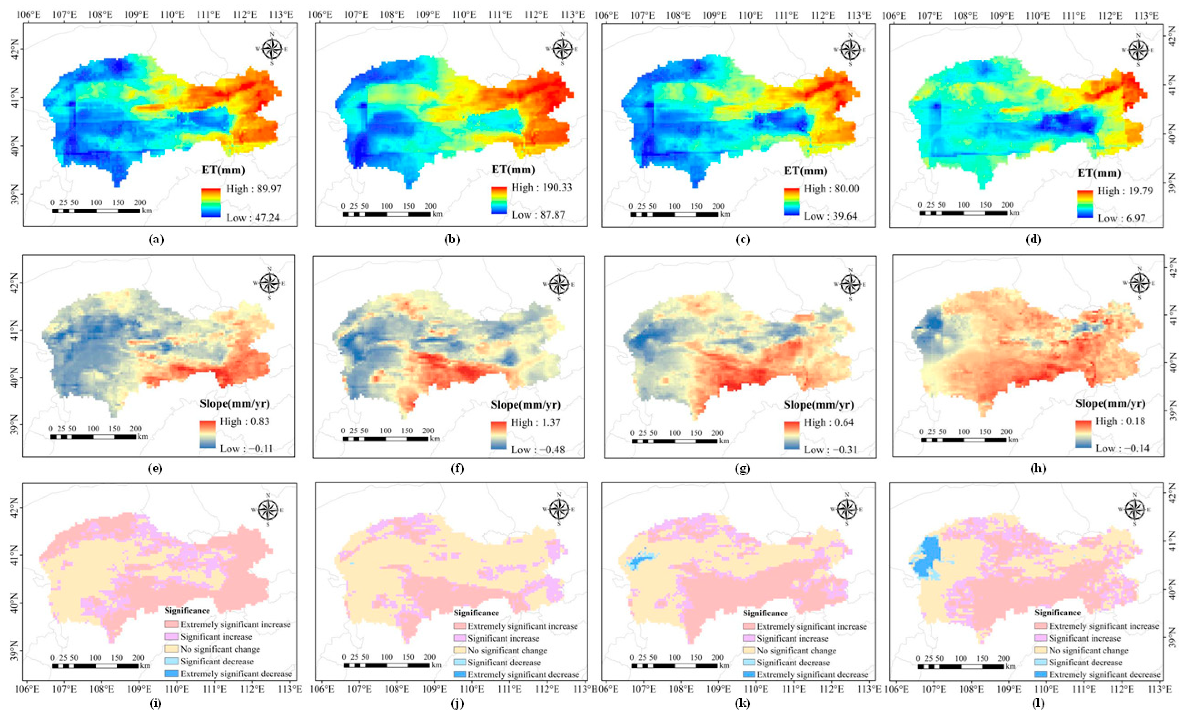
From the interdecadal variations in ET, as the years increase, the region’s low-ET area (blue part) decreased significantly. At the same time, the high-ET area (red part) showed a trend of gradually expanding from east to west and increasing in value, with concentrated areas in Baotou and Ordos (Figure 10a–d). This growth trend was closely related to the evolution of the vegetation cover type and the increase in vegetation coverage. The eastern IMSYRB is part of the key implementation area of China’s ecological protection project. Since 2000, the NDVI in the vicinity of this region has increased significantly, the vegetation has greened, and a large number of grasslands have converted into forests with large ET values. Coupled with global warming and increased precipitation, the ET in these areas has shown rapid growth and a regional expansion trend.
In each decade, the ET trend is not always similar to that of the whole period (Figure 10e–h). The 1980s was the period with the widest range of ET growth and the fastest growth rate. During this period, the temperature and precipitation increased significantly, and the intensification of vegetation transpiration caused the ET growth to accelerate. At the end of the 20th century, the rapid ET growth rate was weakened by the different side changes of precipitation and temperature, and the spatial distribution of the ET change trend was not obvious. After the implementation of the afforestation project in the early 21st century, the ET in most areas in this region showed no significant change due to the drastic fluctuations in temperature and precipitation, especially in low-elevation areas, with a maximum reduction rate of 8.21 mm/yr. However, because of the temperature rise, precipitation increase, and vegetation greening, the ET growth trend in the IMSYRB rebounded over the past 10 years, especially in the western and southern parts of the region.
The multiyear average ET in each season showed a spatial distribution pattern similar to that in the whole period, with high values in the eastern region and low values in the western area (Figure 11). From the variation trends (Figure 11e–h), the ET in each season performed an overall growth trend, with the fastest increase observed in summer (0.34 mm/yr), followed by spring (0.26 mm/yr), autumn (0.16 mm/yr), and winter (0.03 mm/yr). However, the spatial distributions of the ET trends differ slightly among the four seasons. The fastest-growing area of ET in spring was the Hunhe River Basin in the south-eastern study area, and that in the summer and autumn was the southern Ordos region. In winter, ET showed an increasing trend in most areas, and the spatial differences in ET changes were not obvious. The distribution law of the ET change significance in each season was similar to the corresponding change trend (Figure 11i–l). Combined with the statistical results of the significance test (Table 2), spring and winter can be identified as the seasons with the largest areas of ET growth (both significant and extremely significant), accounting for 64.5% and 58.6% of the whole basin, respectively. In summer and autumn, ET did not change significantly (61.9% and 44.9%, respectively).

3.3. Analysis of Factors Influencing ET in the IMSYRB

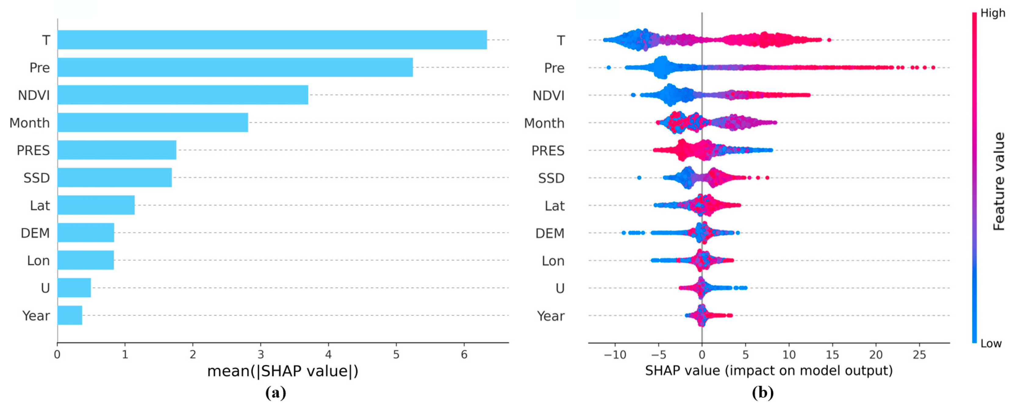
To analyse the contribution and impact direction of each input feature of the RF model to ET results in the IMSYRB, this study calculated the relative importance of each feature in the SHAP environment. Figure 12a shows that temperature was the most important factor affecting ET, followed by precipitation and NDVI. The contribution rates of other characteristics to ET were low, and the effects were not significant. Regarding the direction of influence, the temperature, precipitation, NDVI, sunshine duration, and latitude positively affected ET, the air pressure and wind speed had negative effects, while the longitude had no obvious influence law on the ET direction.
The single-feature dependence graphs shown in Figure 13 further clarify the exact pattern of the contribution of each influencing factor to ET. In general, the main impact values of temperature, precipitation and NDVI identified in SHAP increased monotonically as the variables changed. The SHAP value of the sunshine duration increased with fluctuations, the SHAP value of the air pressure decreased in stages, and the SHAP value of the wind speed decreased monotonously. Specifically, as the monthly average temperature increased, the SHAP main effect value increased, indicating that the positive contribution of temperature to ET was increasing. A temperature of 10 °C was identified as the demarcation point between the negative and positive contributions of temperature to ET. The contribution of precipitation to ET was positive when precipitation was above 25 mm, and when the monthly precipitation reached 200 mm, the main effect value of SHAP tended to become gentle. At this time, a continuous increase in precipitation did not have much of an effect on ET. A positive correlation was found between the NDVI and its SHAP value. When the NDVI value was 0.25, it began to contribute positively to ET. When the NDVI value exceeded 0.5, the slope of the curve became larger, indicating that any further increase in NDVI would cause a greater increment in ET. The relationship between the air pressure and ET decreased in stages. When the air pressure was greater than 880 hPa, the main SHAP effect changed from positive to negative. The sunshine duration is representative of radiative energy, which is positively correlated with its contribution to ET. When the monthly sunshine duration exceeded 250 h, the contribution of this feature to ET changed from negative to positive. A nonlinear negative correlation was identified between the wind speed and its SHAP value. The SHAP main effect value decreased as the wind speed increased until U exceeded 6 m/s. At this time, an increase in wind speed did not further reduce ET.

4. Discussion

4.1. Analysis of ET-Influencing Factors in Arid and Semiarid Areas

The available heat energy introduced by solar radiation provides power for converting the water molecules. The change of water vapour content affects the water vapour cycle between the surface and the atmosphere, thus affecting the evapotranspiration of vegetation [41]. Temperature is a measure of solar radiation energy and was identified as the main factor controlling ET changes in the IMSYRB. This result is the same as that of Zhang et al. [40].
Precipitation is also one of the important driving forces of ET. Especially in arid and semiarid areas, precipitation can largely affect ET by increasing the soil water content and promoting plant growth [42]. In addition, vegetation greening may be the main driving factor affecting the long-term water consumption trend observed in the Yellow River Basin, which is closely related to afforestation activities [43]. The greening of vegetation increases the interception and evaporation of rainfall. Moreover, due to the blocking effect of vegetation on surface runoff, the soil infiltration rate increases, thereby affecting both vegetation transpiration and soil evaporation [44]. Using the VIP model and partial correlation analysis, Bai et al. [43] proved that 56% of the interannual ET variations in the Loess Plateau were driven by the NDVI, and the contribution rate of the NDVI to the ET trend was 93%. In this study, the influence of the NDVI on ET in the IMSYRB was only third among all studied influencing factors, potentially due to the spatial differences in the geographical location and vegetation coverage among the study areas.

4.2. Parameter and Model Selection

The BC2021 model provided good ET simulation results in the IMSYRB (Figure 5) due to its correct interpretation of the land surface hydrothermal process mechanism resulting from the complementary principle and the Budyko equation used to build the model [45]. The important parameter α in the BC2021 model characterizes the relationships between climate factors, vegetation factors, underlying surface characteristics, and hydrological processes. This parameter is the key factor influencing whether the model can accurately estimate ET [46]. In this study, we give this parameter a fixed value of 2.41. However, according to the existing research, due to differences in the underlying surface conditions, the fixed α empirical value may cause large simulation errors, so it must be calibrated and verified for different watersheds. After the test results are qualified, α can be used for subsequent calculations [47]. Because the meteorological data observed at the KBQ05 station were not sufficient to meet the BC2021 requirements for simulating ET in this work, and because the study area was a nonclosed basin, it was difficult to implement a scheme in which measured flux data or the water balance equation were used to calibrate α. Therefore, in this study, we directly substituted the global α value generally recommended by Zhang and Brutsaert to calculate ET. The results show that the outputs of BC2021 with this parameter were satisfactory, further confirming the reliability of the α value of 2.41 when applied to obtain site-scale ET estimations in the IMSYRB.
The RF model exhibited a superior performance in the spatial expansion and variable simulations. Xu et al. [48] compared the application effects of five ML algorithms in upscaling the ET values at flux stations in the Heihe River Basin and found that the uncertainty of RF at the regional scale was slightly lower than that of other models. Based on the RF model, Guo et al. [36] simulated PM2.5 concentrations using ground observation data, AOD, meteorological data, and human factors as auxiliary data across China in 2017 and obtained good results. Hu et al. [15] compared the applicability of physics-based models (SEBS), data-driven models (deep neural networks, random forests, and symbolic regression), and hybrid models in ET simulations. Among them, the RF algorithm showed the best performance. Therefore, in this study, we combined the basic data of the basin and used the RF algorithm to obtain spatially expanded ET values at the site scale.
In addition to its good application performance, another reason for choosing the RF model in this study is that it does not require the input data to be normalized [37]. Normalization solves the problem of increasing the number of iterations when the gradient decreases by scaling the continuous features to the interval of 0–1. Tree models are overstepped and non-derivable and cannot perform gradient descent tasks. Instead, they perform optimization by finding the best splitting point of each feature. Since normalization does not change the position of the split point, it does not affect tree models [49]. In this study, the meteorological, hydrological, and vegetation characteristics, as well as the ET training models corresponding to 23 meteorological stations in the IMSYRB, were first used, and then the characteristics of all grids in the basin were input into the RF algorithm to achieve the goal of simulating regional ET. Normalization limits the range of grid features, preventing them from exceeding the range of the original training set. Therefore, data typically need to be normalized before use; thus, the ML models that use the gradient descent algorithm were not applicable in this study.
When selecting the input features of ML models, scholars have expressed different views due to differences in the study areas, data sources, and selected models [22]. Wen et al. [50] input the maximum temperature, minimum temperature, wind speed, and daily solar radiation into the support vector machine model but found that only using temperature and solar radiation could achieve the best prediction of reference crop evapotranspiration. Granata et al. [21] proved that all the four ML methods achieved the best ET simulation results when the input variables were the net solar radiation, soil heat flux, soil moisture content, wind speed, average relative humidity, and average temperature. Başakın et al. [51] evaluated different combinations of input parameters using support vector machine, adaptive neuro-fuzzy inference system, and artificial neural network models. Their results showed that even when using only global solar radiation data as the input, an increased Bowen ratio system ET prediction accuracy can be obtained. Kisi [52] said that ML models worked better when more input data types were considered. It can be seen that there is no conclusion regarding which input parameter combination optimizes the model simulation effect. Therefore, in this work, we selected 11 features related to the climate, hydrology, topography, and vegetation of the basin to input into the RF model and evaluated the importance of each feature by using the SHAP interpretation framework based on game theory. The evaluation results show that the addition of any feature positively impacts the model simulation results and inputting all features can make the model obtain the best effect. This finding was consistent with the conclusions of Kisi.

4.3. Limitations

While the overall objective has been achieved, several limitations should be focused. First, although various factors have been considered for the establishment of the prediction framework, our results are only dependent on specific parameters. Studies have shown that factors such as soil moisture and solar radiation also act on soil evaporation and vegetation transpiration processes [53,54,55], but due to the limitations of data accuracy and availability, they are not included in the feature set of the ML model in this study. Further, from the perspective of machine learning, we only focus on the accuracy of the output data without benefiting the physical mechanism of the process model. Therefore, improved predictive skills devoid of physical realism may not generalize to unexpected, yet possible, scenarios [56]. We argue that in order to improve the interpretability of ML models and the capability to capture intermediate variables, the gains of a hybrid framework combining physical process models and ML algorithms remain to be explored.

5. Conclusions

In this study, the ET simulation results obtained with the coupled BC2021 model were used to replace the values measured at the flux stations. By combining the basic meteorological and hydrological data of the basin, a hybrid ET prediction framework based on the random forest model was established to predict regional ET in areas lacking measured ET data. This framework was applied to analyse the spatiotemporal ET variations in the IMSYRB from 1982 to 2020, and the SHAP interpretation framework was used to identify the key factors influencing ET in the study area. The main conclusions can be summarized as follows:
  • At the site scale, the ET values estimated by the RF model fit the data measured at the flux stations in the IMSYRB well (R2 = 0.94, MAE = 3.82 mm/mon, and RMSE = 5.07 mm/mon). Spatially, the simulation results show strong correlations with the GLDAS and GLEAM data, with correlation coefficients between 0.77 and 0.97. These results show that the RF model has good numerical simulation and spatial generalization abilities, and the estimated ET has good application potential in hydrological research.
  • From 1982 to 2020, the ET of the IMSYRB ranged from 241.38 mm to 326.37 mm, and the overall ET increased at a rate of 0.80 mm/yr (R2 = 0.23). The average annual ET was 276.39 mm. ET was largest in the summer (140.54 mm), accounting for 50.9% of the year, and the interannual fluctuations in summertime ET were the most obvious.
  • Affected by weather, topography, and vegetation cover, ET showed a regular spatial distribution with high values in the eastern region and low values in the western region. In the past 40 years, the high ET value area gradually expanded from east to west, and the ET values increased. The SLR analysis and T test results showed that approximately 64% of the regions experienced ET growth to different degrees, with the largest increase observed in the 1980s. Summer was the season with the fastest ET changes, with an average change rate of 0.34 mm/yr. The ET growth area was largest in spring, accounting for 64.5% of the whole basin.
  • Temperature, precipitation and NDVI were the most important meteorological factors affecting ET variations in the IMSYRB and played positive roles in promoting ET changes. The contribution rates of the sunshine duration, air pressure, and wind speed to ET were low, and their impacts were not significant.

Author Contributions

Conceptualization, Y.W. and G.W.; methodology, X.J. and J.Y.; validation, Y.W. and Y.A.; formal analysis, X.J.; investigation, J.Y. and B.X.; resources, G.W. and Y.A.; data curation, B.X.; writing—original draft preparation, X.J.; writing—review and editing, G.W. and J.Y.; supervision, B.X. and Y.W.; funding acquisition, G.W. All authors have read and agreed to the published version of the manuscript.

Funding

This study is supported by the National Key Research and Development Program of China, No. 2022YFC3204400, the National Science Fund for Distinguished Young Scholars, No. 52125901, and the National Natural Science Foundation of China, No. 52109001.

Data Availability Statement

Not applicable.

Conflicts of Interest

The authors declare no conflict of interest.

Nomenclature

DEMDigital Elevation ModelKBQ05Hobq Desert 05
EEvapotranspirationMAEmean absolute error
ECeddy covarianceMLMachine learning
EeEquilibrium evaporation termNDVInormalized difference vegetation index
EpaDemand for atmospheric evaporationPreprecipitation
EpoWet surface evapotranspirationPRESair pressure
ETActual evapotranspirationR2Determination coefficient
ETiActual evapotranspiration of period iRFRandom forest
ETmmodel-simulated valueRMSEroot-mean-square error
ET0reference value of actual evapotranspirationSHAPShapley additive explanations
GLDASGlobal Land Data Assimilation SystemSSDsunshine duration
GLEAMGlobal Land Evaporation Amsterdam ModelTtemperature
IDWthe inverse distance weight methodUwind speed
IMSYRBthe Inner Mongolia section of the Yellow River Basinωwater-heat coupled controlling parameter
βctime-varying parameter

References

  1. Wang, K.; Wang, P.; Li, Z.; Cribb, M.; Sparrow, M. A simple method to estimate actual evapotranspiration from a combination of net radiation, vegetation index, and temperature. J. Geophys. Res. Atmos. 2007, 112, D15107. [Google Scholar] [CrossRef]
  2. Xue, B.; Helman, D.; Wang, G.; Xu, C.-Y.; Xiao, J.; Liu, T.; Wang, L.; Li, X.; Duan, L.; Lei, H. The low hydrologic resilience of Asian Water Tower basins to adverse climatic changes. Adv. Water Resour. 2021, 155, 103996. [Google Scholar] [CrossRef]
  3. Jung, M.; Reichstein, M.; Ciais, P.; Seneviratne, S.I.; Sheffield, J.; Goulden, M.L.; Bonan, G.; Cescatti, A.; Chen, J.; de Jeu, R.; et al. Recent decline in the global land evapotranspiration trend due to limited moisture supply. Nature 2010, 467, 951–954. [Google Scholar] [CrossRef] [PubMed]
  4. Fang, Q.; Wang, G.; Zhang, S.; Peng, Y.; Xue, B.; Cao, Y.; Shrestha, S. A novel ecohydrological model by capturing variations in climate change and vegetation coverage in a semi-arid region of China. Environ. Res. 2022, 211, 113085. [Google Scholar] [CrossRef]
  5. Wang, K.; Dickinson, R.E. A review of global terrestrial evapotranspiration: Observation, modeling, climatology, and climatic variability. Rev. Geophys. 2012, 50, RG2005. [Google Scholar] [CrossRef]
  6. Mingyue, C.; Junbang, W.; Shaoqiang, W.; Hao, Y.; Yingnian, L. Temporal and Spatial Distribution of Evapotranspiration and Its Influencing Factors on Qinghai-Tibet Plateau from 1982 to 2014. J. Resour. Ecol. 2019, 10, 213–224. [Google Scholar] [CrossRef]
  7. Chen, J.; Dafflon, B.; Tran, A.P.; Falco, N.; Hubbard, S.S. A deep learning hybrid predictive modeling (HPM) approach for estimating evapotranspiration and ecosystem respiration. Hydrol. Earth Syst. Sci. 2021, 25, 6041–6066. [Google Scholar] [CrossRef]
  8. Zeng, Z.; Peng, L.; Piao, S. Response of terrestrial evapotranspiration to Earth’s greening. Curr. Opin. Environ. Sustain. 2018, 33, 9–25. [Google Scholar] [CrossRef]
  9. Yao, J.; Wang, G.; Jiang, X.; Xue, B.; Wang, Y.; Duan, L. Exploring the spatiotemporal variations in regional rainwater harvesting potential resilience and actual available rainwater using a proposed method framework. Sci. Total Environ. 2023, 858, 160005. [Google Scholar] [CrossRef] [PubMed]
  10. Hu, Z.; Wu, G.; Zhang, L.; Li, S.; Zhu, X.; Zheng, H.; Zhang, L.; Sun, X.; Yu, G. Modeling and Partitioning of Regional Evapotranspiration Using a Satellite-Driven Water-Carbon Coupling Model. Remote Sens. 2017, 9, 54. [Google Scholar] [CrossRef]
  11. Gao, G.; Chen, D.; Xu, C.; Simelton, E. Trend of estimated actual evapotranspiration over China during 1960–2002. J. Geophys. Res. Atmos. 2007, 112, D11120. [Google Scholar] [CrossRef]
  12. Liu, C.; Sun, G.; McNulty, S.G.; Noormets, A.; Fang, Y. Environmental controls on seasonal ecosystem evapotranspiration/potential evapotranspiration ratio as determined by the global eddy flux measurements. Hydrol. Earth Syst. Sci. 2017, 21, 311–322. [Google Scholar] [CrossRef]
  13. Fisher, J.B.; Melton, F.; Middleton, E.; Hain, C.; Anderson, M.; Allen, R.; McCabe, M.F.; Hook, S.; Baldocchi, D.; Townsend, P.A.; et al. The future of evapotranspiration: Global requirements for ecosystem functioning, carbon and climate feedbacks, agricultural management, and water resources. Water Resour. Res. 2017, 53, 2618–2626. [Google Scholar] [CrossRef]
  14. Wang, L.; Wang, G.; Xue, B.; Yinglan, A.; Fang, Q.; Shrestha, S. Spatiotemporal variations in evapotranspiration and its influencing factors in the semiarid Hailar river basin, Northern China. Environ. Res. 2022, 212, 113275. [Google Scholar] [CrossRef] [PubMed]
  15. Hu, X.; Shi, L.; Lin, G.; Lin, L. Comparison of physical-based, data-driven and hybrid modeling approaches for evapotranspiration estimation. J. Hydrol. 2021, 601, 126592. [Google Scholar] [CrossRef]
  16. Liu, Q.; Yang, Z. Quantitative estimation of the impact of climate change on actual evapotranspiration in the Yellow River Basin, China. J. Hydrol. 2010, 395, 226–234. [Google Scholar] [CrossRef]
  17. Carter, C.; Liang, S. Evaluation of ten machine learning methods for estimating terrestrial evapotranspiration from remote sensing. Int. J. Appl. Earth Obs. Geoinf. 2019, 78, 86–92. [Google Scholar] [CrossRef]
  18. Li, J.; Heap, A.D. Spatial interpolation methods applied in the environmental sciences: A review. Environ. Model. Softw. 2014, 53, 173–189. [Google Scholar] [CrossRef]
  19. Li, X.; Liu, S.; Li, H.; Ma, Y.; Wang, J.; Zhang, Y.; Xu, Z.; Xu, T.; Song, L.; Yang, X.; et al. Intercomparison of Six Upscaling Evapotranspiration Methods: From Site to the Satellite Pixel. J. Geophys. Res. Atmos. 2018, 123, 6777–6803. [Google Scholar] [CrossRef]
  20. Wang, X.; Zhong, L.; Ma, Y.; Fu, Y.; Han, C.; Li, P.; Wang, Z.; Qi, Y. Estimation of hourly actual evapotranspiration over the Tibetan Plateau from multi-source data. Atmos. Res. 2023, 281, 106475. [Google Scholar] [CrossRef]
  21. Granata, F. Evapotranspiration evaluation models based on machine learning algorithms—A comparative study. Agric. Water Manag. 2019, 217, 303–315. [Google Scholar] [CrossRef]
  22. Ravindran, S.M.; Bhaskaran, S.K.M.; Ambat, S.K.N. A Deep Neural Network Architecture to Model Reference Evapotranspiration Using a Single Input Meteorological Parameter. Environ. Process. Int. J. 2021, 8, 1567–1599. [Google Scholar] [CrossRef]
  23. Zhang, L.; Brutsaert, W. Blending the Evaporation Precipitation Ratio with the Complementary Principle Function for the Prediction of Evaporation. Water Resour. Res. 2021, 57, e2021WR029729. [Google Scholar] [CrossRef]
  24. Zhang, X.; Wang, G.; Xue, B.; Wang, Y.; Wang, L. Spatiotemporal Variation of Evapotranspiration on Different Land Use/Cover in the Inner Mongolia Reach of the Yellow River Basin. Remote Sens. 2022, 14, 4499. [Google Scholar] [CrossRef]
  25. Tang, G. Digital Elevation Model of China (1 KM). National Tibetan Plateau Data Center. 2019. Available online: https://data.tpdc.ac.cn/en/data/12e91073-0181-44bf-8308-c50e5bd9a734/ (accessed on 30 March 2022).
  26. Bouchet, R.J. Evapotranspiration Potentielle et Evaporation Sous Abri. In Biometeorology; Tromp, S.W., Ed.; Pergamon Press: Oxford, UK, 1962; pp. 540–545. ISBN 978-0-08-009683-4. [Google Scholar]
  27. Zhang, L.; Cheng, L.; Brutsaert, W. Estimation of land surface evaporation using a generalized nonlinear complementary relationship. J. Geophys. Res. Atmos. 2017, 122, 1475–1487. [Google Scholar] [CrossRef]
  28. Hobbins, M.T.; Ramirez, J.A.; Brown, T.C. The complementary relationship in estimation of regional evapotranspiration: An enhanced Advection-Aridity model. Water Resour. Res. 2001, 37, 1389–1403. [Google Scholar] [CrossRef]
  29. Brutsaert, W. A generalized complementary principle with physical constraints for land-surface evaporation. Water Resour. Res. 2015, 51, 8087–8093. [Google Scholar] [CrossRef]
  30. Kim, H.; Kaluarachchi, J.J. Estimating evapotranspiration using the complementary relationship and the Budyko framework. J. Water Clim. Change 2017, 8, 771–790. [Google Scholar] [CrossRef]
  31. Priestley, C.H.B.; Taylor, R.J. On the Assessment of Surface Heat Flux and Evaporation Using Large-Scale Parameters. Mon. Weather Rev. 1972, 100, 81–92. [Google Scholar] [CrossRef]
  32. Liu, X.; Liu, C.; Brutsaert, W. Investigation of a Generalized Nonlinear Form of the Complementary Principle for Evaporation Estimation. J. Geophys. Res. Atmos. 2018, 123, 3933–3942. [Google Scholar] [CrossRef]
  33. Budyko, M.I. The effect of solar radiation variations on the climate of the Earth. Tellus 1969, 21, 611–619. [Google Scholar] [CrossRef]
  34. Li, D.; Pan, M.; Cong, Z.; Zhang, L.; Wood, E. Vegetation control on water and energy balance within the Budyko framework. Water Resour. Res. 2013, 49, 969–976. [Google Scholar] [CrossRef]
  35. Breiman, L. Random Forests. Mach. Learn. 2001, 45, 5–32. [Google Scholar] [CrossRef]
  36. Guo, B.; Zhang, D.; Pei, L.; Su, Y.; Wang, X.; Bian, Y.; Zhang, D.; Yao, W.; Zhou, Z.; Guo, L. Estimating PM2.5 concentrations via random forest method using satellite, auxiliary, and ground-level station dataset at multiple temporal scales across China in 2017. Sci. Total Environ. 2021, 778, 146288. [Google Scholar] [CrossRef]
  37. Li, Y.; Wang, W.; Wang, G.; Tan, Q. Actual evapotranspiration estimation over the Tuojiang River Basin based on a hybrid CNN-RF model. J. Hydrol. 2022, 610, 127788. [Google Scholar] [CrossRef]
  38. Lundberg, S.M.; Lee, S.-I. A Unified Approach to Interpreting Model Predictions. In Proceedings of the Advances in Neural Information Processing Systems 30 (NIPS 2017), Long Beach, CA, USA, 4–9 December 2017; Guyon, I., Luxburg, U.V., Bengio, S., Wallach, H., Fergus, R., Vishwanathan, S., Garnett, R., Eds.; Neural Information Processing Systems (NIPS): La Jolla, CA, USA, 2017; Volume 30. [Google Scholar]
  39. Lundberg, S.M.; Erion, G.; Chen, H.; DeGrave, A.; Prutkin, J.M.; Nair, B.; Katz, R.; Himmelfarb, J.; Bansal, N.; Lee, S.-I. From local explanations to global understanding with explainable AI for trees. Nat. Mach. Intell. 2020, 2, 56–67. [Google Scholar] [CrossRef]
  40. Li, Y.; Fan, J.; Hu, Z.; Shao, Q.; Harris, W. Comparison of evapotranspiration components and water-use efficiency among different land use patterns of temperate steppe in the Northern China pastoral-farming ecotone. Int. J. Biometeorol. 2016, 60, 827–841. [Google Scholar] [CrossRef] [PubMed]
  41. Zhang, Z.; Kang, H.; Yao, Y.; Fadhil, A.M.; Zhang, Y.; Jia, K. Spatial and decadal variations in satellite-based terrestrial evapotranspiration and drought over Inner Mongolia Autonomous Region of China during 1982–2009. J. Earth Syst. Sci. 2017, 126, 119. [Google Scholar] [CrossRef]
  42. Mu, Q.; Zhao, M.; Running, S.W. Improvements to a MODIS global terrestrial evapotranspiration algorithm. Remote Sens. Environ. 2011, 115, 1781–1800. [Google Scholar] [CrossRef]
  43. Bai, M.; Mo, X.; Liu, S.; Hu, S. Contributions of climate change and vegetation greening to evapotranspiration trend in a typical hilly-gully basin on the Loess Plateau, China. Sci. Total Environ. 2019, 657, 325–339. [Google Scholar] [CrossRef]
  44. He, Z.; Jia, G.; Liu, Z.; Zhang, Z.; Yu, X.; Xiao, P. Field studies on the influence of rainfall intensity, vegetation cover and slope length on soil moisture infiltration on typical watersheds of the Loess Plateau, China. Hydrol. Process. 2020, 34, 4904–4919. [Google Scholar] [CrossRef]
  45. Lhomme, J.-P.; Moussa, R. Matching the Budyko functions with the complementary evaporation relationship: Consequences for the drying power of the air and the Priestley–Taylor coefficient. Hydrol. Earth Syst. Sci. 2016, 20, 4857–4865. [Google Scholar] [CrossRef]
  46. Zhou, S.; Yu, B.; Huang, Y.; Wang, G. The complementary relationship and generation of the Budyko functions. Geophys. Res. Lett. 2015, 42, 1781–1790. [Google Scholar] [CrossRef]
  47. Yang, D.; Sun, F.; Liu, Z.; Cong, Z.; Ni, G.; Lei, Z. Analyzing spatial and temporal variability of annual water-energy balance in nonhumid regions of China using the Budyko hypothesis. Water Resour. Res. 2007, 43, W04426. [Google Scholar] [CrossRef]
  48. Xu, T.; Guo, Z.; Liu, S.; He, X.; Meng, Y.; Xu, Z.; Xia, Y.; Xiao, J.; Zhang, Y.; Ma, Y.; et al. Evaluating Different Machine Learning Methods for Upscaling Evapotranspiration from Flux Towers to the Regional Scale. J. Geophys. Res. Atmos. 2018, 123, 8674–8690. [Google Scholar] [CrossRef]
  49. Douna, V.; Barraza, V.; Grings, F.; Huete, A.; Restrepo-Coupe, N.; Beringer, J. Towards a remote sensing data based evapotranspiration estimation in Northern Australia using a simple random forest approach. J. Arid Environ. 2021, 191, 104513. [Google Scholar] [CrossRef]
  50. Wen, X.; Si, J.; He, Z.; Wu, J.; Shao, H.; Yu, H. Support-Vector-Machine-Based Models for Modeling Daily Reference Evapotranspiration with Limited Climatic Data in Extreme Arid Regions. Water Resour. Manag. 2015, 29, 3195–3209. [Google Scholar] [CrossRef]
  51. Başakın, E.E.; Ekmekcioğlu, Ö.; Özger, M.; Altınbaş, N.; Şaylan, L. Estimation of measured evapotranspiration using data-driven methods with limited meteorological variables. Ital. J. Agrometeorol. 2021, 2021, 63–80. [Google Scholar] [CrossRef]
  52. Kişi, Ö. Daily pan evaporation modelling using a neuro-fuzzy computing technique. J. Hydrol. 2006, 329, 636–646. [Google Scholar] [CrossRef]
  53. Wang, Y.; Zhang, Y.; Yu, X.; Jia, G.; Liu, Z.; Sun, L.; Zheng, P.; Zhu, X. Grassland soil moisture fluctuation and its relationship with evapotranspiration. Ecol. Indic. 2021, 131, 108196. [Google Scholar] [CrossRef]
  54. Cunha, A.C.; Filho, L.R.A.G.; Tanaka, A.A.; Goes, B.C.; Putti, F.F. Influence of the estimated global solar radiation on the reference evapotranspiration obtained through the penman-monteith FAO 56 method. Agric. Water Manag. 2021, 243, 106491. [Google Scholar] [CrossRef]
  55. Brust, C.; Kimball, J.S.; Maneta, M.P.; Jencso, K.; He, M.; Reichle, R.H. Using SMAP Level-4 soil moisture to constrain MOD16 evapotranspiration over the contiguous USA. Remote Sens. Environ. 2021, 255, 112277. [Google Scholar] [CrossRef]
  56. Bhasme, P.; Vagadiya, J.; Bhatia, U. Enhancing predictive skills in physically-consistent way: Physics Informed Machine Learning for hydrological processes. J. Hydrol. 2022, 615, 128618. [Google Scholar] [CrossRef]
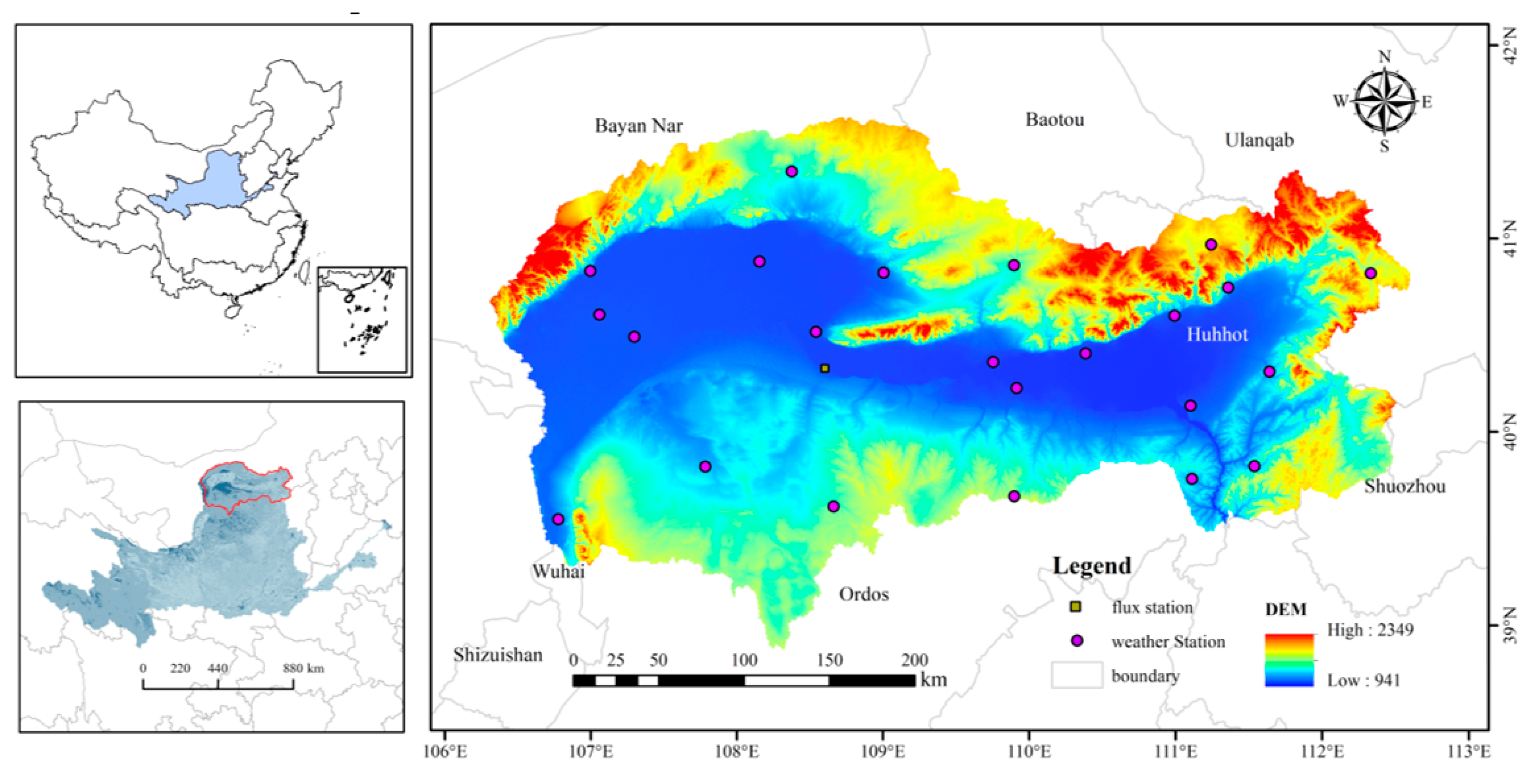
Figure 1. Geographical location and distribution of observation sites in the Inner Mongolia section of the Yellow River Basin (IMSYRB).
Remotesensing 15 02234 g001
Figure 2. Research framework and methods.
Remotesensing 15 02234 g002
Figure 3. Comparison between the simulated ET by the BC2021 model and the observed ET recorded at the KBQ05 station: (a) changes over time; (b) fitting degree.
Remotesensing 15 02234 g003
Figure 4. Influence of hyperparameters on the modelling results obtained with the RF algorithm: (a) n_eatimators; (b) max_features; (c) max_depth; (d) min_samples_split; (e) min_samples_leaf.
Remotesensing 15 02234 g004
Figure 5. Comparisons between the extracted and measured values of each dataset at the KBQ05 station: (a) changes over time; (b) fitting degree.
Remotesensing 15 02234 g005
Figure 6. Spatial distributions of the correlation coefficients between the RF simulation results and remote sensing data: (a) GLEAM and (b) GLDAS.
Remotesensing 15 02234 g006
Figure 7. Interannual variations in ET in the IMSYRB from 1982 to 2020.
Remotesensing 15 02234 g007
Figure 8. Annual variation in ET in the IMSYRB from 1982 to 2020.
Remotesensing 15 02234 g008
Figure 9. Spatial variation in annual ET in the IMSYRB from 1982 to 2020: (a) multiyear average ET, (b) multiyear change trend of ET, and (c) significant change trend of ET.
Remotesensing 15 02234 g009
Figure 10. Interdecadal spatial distribution and variation trend of ET in the IMSYRB from 1982 to 2020: spatial distribution from (a) 1982–1990, (b) 1991–2000, (c) 2001–2010, and (d) 2011–2020; trends from (e) 1982–1990, (f) 1991–2000, (g) 2001–2010, and (h) 2011–2020.
Remotesensing 15 02234 g010
Figure 11. Spatial variation in ET in the IMSYRB from 1982 to 2020: (ad) multiyear average ET in Spring, Summer, autumn and winter, (eh) multiyear ET trend in four seasons, and (il) significant ET trend in four seasons.
Remotesensing 15 02234 g011
Figure 12. Effects of RF input factors on ET: (a) global importance map; (b) feature summary graph.
Remotesensing 15 02234 g012
Figure 13. SHAP-dependent feature graphs: (a) temperature; (b) precipitation; (c) NDVI; (d) air pressure; (e) sunshine duration; (f) wind speed.
Remotesensing 15 02234 g013
Table 1. Information of the data involved in this study.
VariableDataset NameTime RangeTemporal ResolutionSpatial Resolution
DEMChina 1-km digital elevation map1982–2020-1 km
Pre, T, U, SSD, PRESChina daily surface climate dataset (V3.0)1982–2020Daily-
NDVIA 5-km-resolution dataset of the monthly NDVI product of China (1982–2020)1982–2020Monthly5 km
ETEddy covariance flux station data2006–200930 min-
ETGLEAM1982–2020Monthly0.25° × 0.25°
ETGLDAS1982–2020Monthly0.25° × 0.25°
Table 2. ET change trend significance test statistical results.
Standard of ClassificationET Variation TrendProportion (%)
SlopepAnnualSpringSummerAutumnWinter
Slope > 0p < 0.01Extremely significant increase49.545.421.337.338.2
0.01 ≤ p < 0.05Significant increase14.519.116.816.420.4
p > 0.05No significant change35.835.561.944.936.3
Slope < 00.01 ≤ p <0.05Significant decrease0.20.00.00.91.7
p < 0.01Extremely significant decrease0.00.00.000.63.4
Disclaimer/Publisher’s Note: The statements, opinions and data contained in all publications are solely those of the individual author(s) and contributor(s) and not of MDPI and/or the editor(s). MDPI and/or the editor(s) disclaim responsibility for any injury to people or property resulting from any ideas, methods, instructions or products referred to in the content.