Abstract
Crop residue cover is vital for reducing soil erosion and improving soil fertility, which is an important way of conserving tillage to protect the black soil in Northeast China. How much the crop residue covers on cropland is of significance for black soil protection. Landsat-8 and Sentinel-2 images were used to estimate corn residue coverage (CRC) in Northeast China in this study. The estimation model of CRC was established for improving CRC estimation accuracy by the optimal combination of spectral indices and textural features, based on soil texture zoning, using the random forest regression method. Our results revealed that (1) the optimization C5 of spectral indices and textural features improves the CRC estimation accuracy after harvesting and before sowing with determination coefficients (R2) of 0.78 and 0.73, respectively; (2) the random forest improves the CRC estimation accuracy after harvesting and before sowing with R2 of 0.81 and 0.77, respectively; (3) considering the spatial heterogeneity of the soil background and the usage of soil texture zoning models increase the accuracy of CRC estimation after harvesting and before sowing with R2 of 0.84 and 0.81, respectively. In general, the CRC estimation accuracy after harvesting was better than that before sowing. The results revealed that the corn residue coverage in most of the study area was 0.3 to 0.6 and was mainly distributed in the Songnen Plain. By the estimated corn residue coverage results, the implementation of conservation tillage practices is identified, which is vital for protecting the black soil in Northeast China.
1. Introduction
As one of the most valuable natural resources, soils provide about 98.8% of human food [1]. The Northeast Plain of China is one of the three major black soil regions in the world [2], with the characteristics of good physicochemical properties and high fertility [3], covering a total area of about 1.09 million km2 and accounting for 16% of China’s total crop yield [4]. Unfortunately, long-term intensive cultivation and a lack of effective protection have led to the degradation of the soil structure, decreasing soil organic content and increasing soil erosion [5]. One important way to protect the soil is conservation tillage [6]. Leaving the crop residue on the soil surface after harvesting is a recommended conservation tillage practice [7,8,9]. Crop residue cover can significantly contribute to the protection of cropland from wind and water erosion, as well as reduce evapotranspiration. Furthermore, long-term crop residue cover returning to cropland can increase soil organic carbon and improve the physical structure of the soil further, and this plays an important role in soil conservation and sustainable development. Moreover, crop residue cover is an important component of agroecosystems, influencing the flow of water, carbon, nitrogen, and energy cycles [10]. Crop residue cover can effectively reduce air pollution and harmful gas emissions by avoiding crop residue burning [11,12]. Crop residue cover is not only an indicator for monitoring conservation tillage practices [13], but also an important input for terrestrial ecosystem carbon modeling [14], which is crucial for surface carbon cycle modeling. Accurate estimations of crop residue cover can not only provide insight into the effects of conservation tillage and aid agricultural production, but also serve as an input for carbon cycle modeling. Therefore, this study aims to estimate the crop residue cover in the region of Northeast China accurately and efficiently using remote sensing techniques.
Corn is a dominant crop in the black soil of Northeast China, with large amounts of corn residue left in cropland after harvesting as a common method of conservation tillage [15]. The traditional ways of estimating corn residue coverage (CRC) include visual judgment or measuring using a band tape. These measuring methods are simple but are subjective, time consuming, and laborious. Therefore, it is difficult to use direct measuring methods to estimate the CRC accurately and efficiently in a regional area [16,17,18]. Fortunately, remote sensing is one way of acquiring land surface information quickly and efficiently on a regional scale. Many researchers have used remote sensing images for CRC estimation [19].
One difficulty in crop residue coverage estimation by remote sensing is that the crop residue has similar spectral characteristics to the soil background, with only the lignin and cellulose within crop residues having strong absorption valleys around 2100 nm [20]. Given these spectral characteristics of crop residue in short-wave infrared (SWIR) bands, many researchers have built spectral indices for CRC estimation, such as the cellulose absorption index (CAI) [21], the normalized difference tillage index (NDTI), the simple tillage index (STI), and the normalized difference residue index (NDRI) [22,23]. However, the spectral indices have some limitations for estimating CRC because the reflectance of crop residue is influenced by numerous crop factors, including moisture content, content of lignin, cellulose, and hemicellulose [13,23,24]. Moreover, the regression model established by a single tillage index cannot fully reflect the influence of spatial heterogeneity, and each tillage index has its limitations, leading to the disadvantages of low prediction accuracy and poor stability of the model. Some researchers have found that textural features can help to distinguish the differences in CRC, which can depict the spatial variations of image brightness and provide more distinguishing information for CRC monitoring. The study results of Najafi [19] and Xiang [25] revealed that the combination of spectral indices and texture features can be used to improve the accuracy of CRC estimation.
In recent years, with the development of computer technology, machine learning methods have been explored to improve CRC estimation performance. Ding [26] uses a machine learning approach to estimate CRC by combining spectral indices and texture features. Yue and Tian [27] use a random forest algorithm to estimate fractional vegetation cover, CRC, and bare soil cover on arable land using a Sentinel-2 MSI image. Another issue that needs to be pointed out is that most spectral indices are affected by the soil background, such as soil texture, soil organic content, and soil water content, resulting in unreliable CRC estimation results in regional areas and the challenge of guaranteeing the robustness in large areas with obvious variations in the soil background. Moreover, the CRC will decompose and decay gradually from harvesting to sowing in the next year, which will affect the reflectance of the CRC. Therefore, we should explore the development of specific modelling for estimating CRC after harvesting and before sowing. Most studies on CRC are still limited to small regional scales rather than large scales [9,28]. When the study area is small, the straw cover is very close within the study area, resulting in similar straw cover characteristics and types [29]. Therefore, the model constructed in this particular study area, although it produces good estimates, still has limitations. It may not be applicable to other areas that differ significantly from the study area in terms of geographic location and climate type.
This study aims to improve CRC estimation after harvest and before sowing by combining the spectral indices and textural features of Landsat-8 and Sentinel-2 images in Northeast China. To reduce the effects of soil background, it uses a soil texture zoning model. To enhance computational efficiency on a regional scale, it employs the Google Earth Engine cloud computing platform. The specific objectives are (1) to build optimized image features, including spectral indices and textural features, for the creation of random forest trees; (2) to explore the potential of random forest and multiple linear regression for CRC estimation; (3) to solve the problem of heterogeneous soil background by using a soil texture zoning model during CRC estimation; (4) to develop optimized models for CRC estimation after harvest and before sowing using optimized features and random forests by considering soil texture difference.
2. Materials and Methods
2.1. Study Area
Northeast China is located from 118°53′E, 38°43′N to 135°5′E, 53°33′N, covering 1.09 million km2, and consists of Liaoning Province, Jilin Province, and Heilongjiang Province. Zoning from the China Agro-climate Zoning Scheme, Northeast China can be divided into six agro-climate sub-zones, namely, Greater Khingan Mountain Zone (GKM), Lesser Khingan Mountain Zone (LKM), Changbai Mountain Zone (CM), Sanjiang Plain Zone (SJP), Liaoning Plain and Hilly Zone (LPH), and Songnen Plain Zone (SNP). The location, topography, and six agricultural sub-areas of Northeast China are shown in Figure 1. The farmland in Northeast China is dryland mainly, and the dominant crop types are corn, soybean, and paddy rice, which account for more than 90% of the total crop planting area in Northeast China [30]. Among these three crops, the planting area of corn is the largest in Northeast China, accounting for 26.6% of China’s corn planting area. Additionally, annual corn production accounts for about 1/3 of China’s total corn production, ranking first in China. The growing season of corn in Northeast China is from mid-May to early October [31], and the CRC period ranges from the end of October to the end of April. Additionally, the phonologies of corn, paddy rice, and soybean in Northeast China are shown in Table 1.
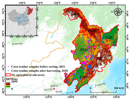
Figure 1.
Location, topography, and six agricultural sub-areas of Northeast China.

Table 1.
The phenology of crops in Northeast China.
2.2. Data Sources and Preprocessing
2.2.1. Corn Residue Samples
The samples with varied coverage were collected for CRC modeling and for the validation of CRC estimation, and were collected randomly and distributed as evenly as possible in the corn growing areas of the whole Northeast China. There were a total of 610 samples (100 sampling points from field observation, and 510 sampling points from Google Earth), and 70% of them were used for training and 30% of them were used for validation. These samples came from field campaigns and very high spatial resolution satellite images of Google Earth (GE).
- (1)
- Field measurements
There were two field campaigns carried out for collecting CRC samples in November 2020 (after harvesting) and April 2021 (before sowing in the next growing season). For matching the spatial resolution of Landsat-8 images (30 m), 100 quadrats with a size of 30 m × 30 m with varied CRC levels were collected in field campaigns (Figure 1). In each quadrat, there were 5 photos taken around the four corners and the center of the quadrat. Furthermore, these 5 photos covered the dense and sparse residuals equally if there was obvious spatial heterogeneity in the measured quadrat. For each photo, there were two ropes marked at 1 m intervals, which were used for the corn residue measurement. In the field measurement, we used cellphones to take photos at a height roughly around 1.5 m above the ground (Figure 2). To avoid significant residue shadows covering soils, all photos were taken at a local time of 8:30 a.m.–4:30 p.m. For minimizing the shadow effect, we tried to take the photos backing the sun, where the viewing angle was near to the sun’s direction. The locations of all samples were acquired using a Huace i80 real-time kinematic (RTK) GPS receiver (Huace Ltd., Shanghai, China). In addition, a fixed-wing drone named P330 Pro was used to collect corn residue samples covering Quanyangou Village on 11 November 2020. There were 8 samples collected from UAV images, which acted as samples from field work.
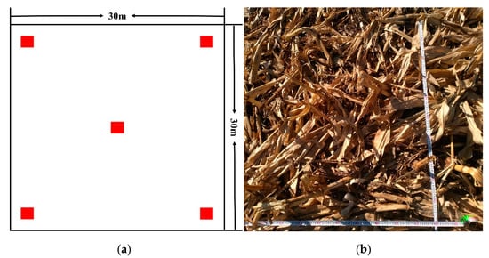
Figure 2.
The basic sample unit (30 m × 30 m) (a), and the measurement of CRC for each subplot (1 m × 1 m) (b).
- (2)
- Google Earth collection
In addition to the photos taken in the field campaign, there were additional samples collected from the very-high-resolution Google Earth imagery, and the samples were acquired through the semi-automated visual interpretation method. Based on the maximum NDTI composite during the sampling period, the samples were distributed by random stratified sampling into areas of 90 × 90 m (Figure 3b). Since corn residue in the study region is usually brighter than surrounding vegetation and soil, we used the method of maximum variance between two classes (OSTU, named by Japanese Nobuyuki otsu) to distinguish the corn residue from non-residue (Figure 3c) [32]. However, there is less color difference between the corn residue and the non-residue, so the collect earth online tool was used to calculate the CRC in these regions. This tool is a free open-source software for land monitoring developed by the Food and Agriculture Organization of the United Nations (FAO) [33]. Additionally, based on a 90 × 90 m square plot, 49 points of 2 × 2 m were scattered evenly in this quadrat, and these points were used to observe presence/absence of corn residue by visual interpretation (Figure 3d). In each quadrat, three independent experts with local experience provided visual interpretation of the image to estimate the corn residue coverage, and the reference information from experts was subsequently averaged. The criteria for sample collection were that (1) the acquisition time of the selected sampling points in each agricultural area should be within the time frame of Landsat-8 and Sentinel-2 remote sensing imagery; (2) all selected sample points should be distributed evenly within the study area as far as possible; (3) the collected samples should have varied CRC values.

Figure 3.
Illustration of the CRC assessment method using thresholding of Google Earth imagery: (a) Google Earth image chip, (b) 90 × 90 m Google Earth image chip, (c) CRC obtained by thresholding, (d) CRC collected on the Collect Earth sample collector.
2.2.2. Soil Data
Soil texture data were downloaded from the International Soil Reference and Information Centre (ISRIC) (https://soilgrids.org/, accessed on 1 March 2023), and a raster dataset covering the surface soil texture in the study area was used to quantify the sand content and clay content raster in topsoil (0–5 cm) with the spatial resolution of 250 m. The soil type map on the scale of 1:1,000,000 was acquired from the Resource Environment Data Cloud Platform (http://www.resdc.cn, accessed on 1 March 2023) from the Second National Soil Census.
2.2.3. Remote Sensing Images
Landsat-8 and Sentinel-2 images acquired after harvesting from October to November 2020, and before sowing from March to May 2021, were used for constructing a CRC estimation model. The acquisition dates of these satellite remote sensing images are shown in Table 2. All Landsat-8 and Sentinel-2 images were processed in the Google Earth Engine cloud platform for radiometric correction, atmospheric correction, and geometric correction. A single image dataset cannot cover the whole study area efficiently and completely; therefore, both the Landsat-8 and Sentinel-2 images were used in this study, and the image acquisition periods are listed in Table 2. Considering the spectral and spatial differences between Landsat-8 and Sentinel-2 images, these two kinds of images were harmonized using conversion factors referenced by Chastain et al. [34]. To prevent green vegetation from influencing CRC estimates, this study used NDVI > 0.3 to mask green vegetated farmland and set different satellite transit times for different agro-climatic zones [35]. Little to no rain (less than 0.25 cm) had fallen the week before the image transit, and the soil moisture levels were constantly dry.

Table 2.
Acquisition dates of Landsat-8 and Sentinel-2 images used in this study.
2.3. Methods
The flowchart used for CRC estimation in this study is available in Figure 4. There are three steps for CRC estimation, including corn residue sample collection, CRC estimation model building, and model validation. During the CRC estimation modeling, the optimization of image features, including spectral indices and textural features, and the comparison of multiple linear regression and random forest were performed.
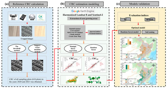
Figure 4.
The flowchart used for CRC estimation in this study.
2.3.1. Spectral Indices and Textural Features
Because of the good performance of spectral indices in CRC estimation, seven spectral indices (Table 3) were used for CRC estimation in this study. In addition, the textural features, including mean, variance, homogeneity, contrast, dissimilarity, entropy, second moment, and correlation, were used for CRC estimation.

Table 3.
Spectral indices used for CRC modeling.
- (1)
- Spectral indices
Considering the spectral sensitivity to corn residue, the Green, Red, NIR, SWIR1, and SWIR2 bands of Landsat-8 and Sentinel-2 images were used to calculate the spectral indices, including normalized difference tillage index (NDTI), normalized difference index 5 (NDI5), normalized difference index 7 (NDI7), normalized difference senescent vegetation index (NDSVI), simple tillage index (STI), modified crop residue cover (MCRC), and normalized difference residue index (NDRI). Table 3 shows the calculation and references of these spectral indices.
- (2)
- Textural features
We used the textural features to estimate CRC accurately in this study because of the distinct textural differences of corn residues with different coverage and different methods of ridging management. Therefore, the textural features were used to estimate CRC accurately in this study. The grey-level co-occurrence matrix (GLCM) developed by Haralick [40] is a popular algorithm for extracting textural features from remotely sensed imagery [41,42,43]. Additionally, the GLCM approach was used to depict the textural characteristics of different CRC in this study. There are eight GLCM textural features, including mean, variance, homogeneity, contrast, dissimilarity, entropy, second moment, and correlation [44], that were used for depicting the textural difference of corn residue in this study. These statistical indicators can quantify the local texture structure of an image from different perspectives while reflecting the differences in the spatial characteristics of the features. The extraction of texture features relies heavily on the local variation in the image’s grey level and the window size for calculating the co-occurrence matrix. Considering the size and direction of cropland covered with corn residue, a window size of 3 × 3 pixels, a moving step of 1 pixel, and a moving direction of 45° were used for CRC estimation in this study [25,45].
2.3.2. CRC Estimating Models
The CRC estimation model has been developed by the multiple linear and random forest approaches using spectral indices, textural features, and a combination of them for estimating the CRC in Northeast China. Additionally, the estimation accuracy can be assessed using the R2 and RMSE error.
- (1)
- Multiple Linear Regression model
Multiple linear regression is a common statistical model that uses multiple independent variables to explain changes in the dependent variable. Considering there is a good correlation between the spectral indices and textural features with CRC, the multiple linear regression model was used to explore the relationship between remote sensing indices and CRC in this study. The multiple linear regression model of CRC estimation is given by the following:
where y is the dependent variable, which is the estimated result of CRC in this study; (i = 1, 2, …, k) are the k independent variables, which are the spectral indices and textural features in this study; (i = 0, 1, 2, …, k) is the k + 1 regression coefficient; and ξ is the random error term [46].
In the multiple linear regression model, the sensitivities of independent variables () are different. Therefore, the correlations between spectral indices and textural features with the CRC were assessed first. Additionally, the spectral indices and textural features with high correlation were used to develop the estimation model. Secondly, a further covariance diagnosis was then performed to select the posterior variables, and the final variables were determined by stepwise regression. Finally, three regression estimation models were built using the spectral indices, textural features, and combinations of spectral indices with textural features.
- (2)
- Random forest regression model
Random forest is a machine learning algorithm based on multiple decision trees that can be used for regression and classification. Additionally, the decision trees are trained using the training samples and built independently. Each decision tree provides a classification result for the input data during the classifying process. Additionally, all the classification results should be collected and the prediction with the most vote will act as the final classification result. Essentially, a random forest enables a large number of weak or weakly correlated classifiers to form a strong classifier. Random forest tends to outperform most traditional machine learning classification methods in terms of accuracy. The random forest approach can deal with high-dimensional data effectively. In addition, the random forest regression is extremely adaptive and resistant to noise [47]. It can not only process more input variables but can also obtain reasonable prediction accuracy when there are fewer input variables [48]. Therefore, we used random forest to estimate CRC using spectral indices, textural features, and their combinations in this study. We measured CRC as the target value to build a random forest model. The training samples were divided into training and validation sets, and the optimal parameters were found by searching the grid, comparing the accuracy of the validation set with different parameters, and finally determining the values of several important parameters in the random forest model: the number of decision trees is 300 and the depth is 10.
2.3.3. Soil Texture Zoning
There are several kinds of soil types with high spatial heterogeneity in the study area, and the black soils and sandy soil are two dominant soil types with significant differences in both physicochemical characteristics and spectral background. The black soil is dark, clayey, and rich in organic content. The sandy soil is bright, sandy, and poor in water retention capacity. The different physicochemical properties of varied soil types lead to significant spectral differences, which make CRC estimation difficult. To improve the CRC estimation, we developed the soil texture zoning method to quantify the differences and variations in soil background for CRC estimation. We classified the cropland with a proportion of sand particles in topsoil (0–5 cm) of more than 39% as sandy soil zones [49], while we classified the cropland with a proportion of sand particles in topsoil (0–5 cm) of less than 39% as clayey soil zones. Figure 5 shows the proportions of sand particles and particles.
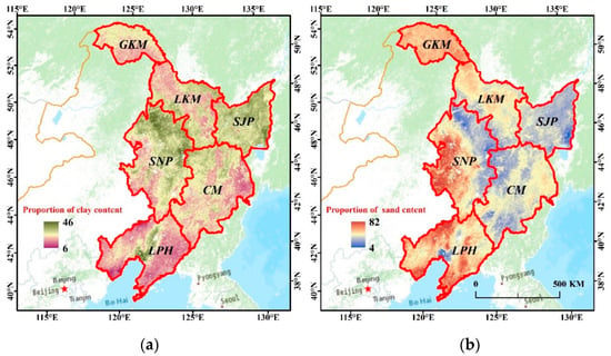
Figure 5.
Proportions of clay particles (a) and sandy particles (b) in the study area.
2.3.4. OTSU Threshold Segmentation for CRC Sampling
Sample collection and optimization are very important for CRC estimation using random forest. There are two kinds of sampling: one which involves segmenting the photos taken in field campaigns and another which involves segmenting the clipped high-spatial-resolution images from Google Earth. Considering its advantages of being adaptive, robust, and easy to use, the binarized OSTU algorithm [32] was used to segment the corn residue and background soil pixels for collecting CRC samples from photos taken in field campaigns and high-spatial-resolution remote sensing images. The optimal threshold value was determined adaptively by the maximum variance between corn residue pixels and non-corn residue pixels for each photo and each clipped image using the OSTU segmentation method firstly. Then, all the pixels were classified into two classes: corn residue and non-corn residue. Then, the ratio between the number of segmented corn residue covered pixels to the total number of pixels in the given clipped image or photo was obtained for the corn residue coverage calculation. We calculated all the photos and clipped images, and we used the calculated results as samples for CRC estimation.
2.3.5. Validation of Residue Cover Estimation
Validation was performed for the two procedures, corn type classification and CRC estimation, in this study. Additionally, the validation and accuracy assessment of corn type classification were performed using Overall Accuracy (OA), User’s Accuracy (UA), Producer’s Accuracy (PA), and F1 score (F1). In the validation of CRC estimation, the measured data were compared with the predicted values from the optimized multiple linear regression model and random forest model. Additionally, the determination coefficient (R2) and the root mean square error (RMSE) [50] were used for validation as follows:
where is the number of correctly classified pixels for class i; N is the total number of all pixels; and are the sum of the elements in row i and column i of the confusion matrix, respectively; is the measured CRC; and is the estimated CRC using a multiple linear regression model and random forest model.
3. Results and Analysis
3.1. Collected CRC Samples Using the OSTU Method
There were 610 samples used for CRC modeling in this study, which were obtained from field photos and clipped images from Google Earth. All the photos and clipped images were used for calculating the CRC value using the OSTU method. Figure 6 shows the segmented result of photos ((a) to (c)) and clipped images ((d) to (f)). For the segmented results of photos, the segmented details using OSTU (shown in (b)) are better than those using a support vector machine (shown in (c)). Similarly, there are almost the same segmented results for corn residue cover using the OSTU method (e) and support vector machine (f) for a clipped high-resolution image from Google Earth. Considering the trade-off between classification efficiency and accuracy, this study chose the OSTU threshold segmentation method for CRC sample collection from photos and clipped images.
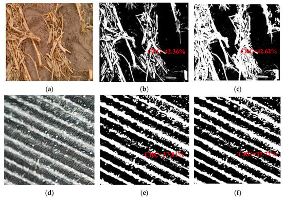
Figure 6.
Examples of collected CRC samples using the OSTU method from photos taken in field campaign (a–c) and high-resolution images collected from Google Earth (d–f).
3.2. Classified Result of Corn Planted Area
Before estimating the CRC, this study classified the corn planting area in Northeast China, which has a large inter-annual variation in crop cultivation structure. The samples of four field campaigns were used in corn planting area classification. Furthermore, the transferred samples from 2017–2019 in the published classification work of You [30] were used for producing the crop classification map for 2020 in Northeast China [51]. The random forest model and feature optimization algorithm were used to identify the three main crop types of rice, corn, and soybean in the study area on the Google Earth Engine platform. Figure 7 shows that the classification results are consistent with the actual spatial distribution of land types visually. In addition, the quantitative results reveal a good classification result with a Kappa coefficient of 0.93 and an OA of 0.96. Among these three main crops in the study area, there is the highest accuracy for paddy rice, with a UA of 0.98, F1 score of 0.98, and PA of 0.98. The classification accuracy of corn is slightly lower, with a UA of 0.96, F1 score of 0.97, and PA of 0.98. Additionally, the classification accuracy of soybean is the lowest, with a UA of 0.87, F1 score of 0.79, and PA of 0.73.
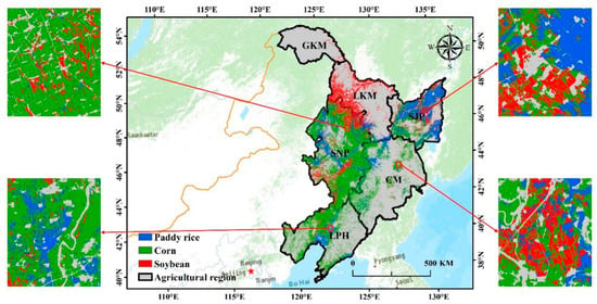
Figure 7.
Crop type classification results in the growing season of 2020.
Corn is the main crop in the study area, which is distributed mainly in the SNP and LPH, while rice is mainly distributed in the SJP, and soybean is more widely distributed in the northern SNP. There is mostly forest in the GKM and LKM, so they were not involved in the calculation of subsequent estimations of CRC.
3.3. Optimization of Spectral Indices and Textural Features
The optimized combinations of spectral indices and textural features for CRC estimation were used in this study. Table 4 showed the R2 of these features with the measured CRC after harvesting and before sowing. NDTI and STI had high correlations with CRC after harvesting (R2 0.64, p < 0.01). Before sowing, STI had the highest R2 of 0.61 and RMSE of 0.12, followed by NDTI with an R2 of 0.60 and RMSE of 0.12. The coefficient of determination after harvest was higher than that before sowing for all seven spectral indices. Figure 8 shows the corrections between NDTI and STI with measured CRC after harvesting (a) and before sowing (b). One possible reason for the lower CRC estimation accuracy before sowing is that the spectrum was a mixture of corn residue and background soil, as corn residue decomposes gradually from harvesting to sowing in the next growing season [25].

Table 4.
Coefficient of determination between spectral indices and measured CRC.
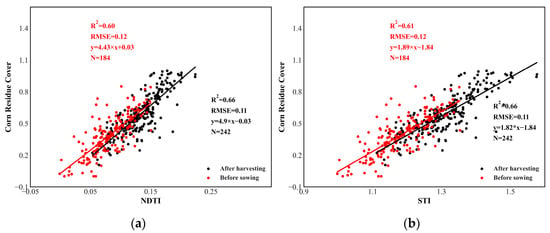
Figure 8.
Coefficient of determination between NDTI and STI with measured CRC after harvesting (a) and before sowing (b).
This study also used eight texture feature metrics (mean, variance, homogeneity, contrast, dissimilarity, entropy, second moments, and correlation) to estimate CRC. However, Table 4 shows that the coefficient of determination between these features and CRC was low in all cases. The best-performing texture feature after harvesting was NIR_mean, with an R2 of 0.33 and RMSE of 0.15. Among the texture features, NIR_mean, Blue_mean, Red_mean, and Green_mean had relatively better performance than the others (see Table 4). This suggests that texture features are less effective than spectral indices for CRC estimation.
Fortunately, combining optimized spectral indices and optimized textural features improves the coefficient of determination between the image features and measured CRC. Table 5 shows the coefficient of determination between the estimated and measured CRC by combining different features. The results indicate that the estimation accuracy by combining the four spectral indices of NDTI, STI, NDI7, and NDRI is significantly improved, with an R2 value of 0.74 after harvesting and 0.71 before sowing, while the estimation accuracy by combining the spectral indices of NDTI, STI, NDI7, NDRI, NDI5, MCRC, and NDSVI is 0.75 after harvesting and 0.73 before sowing. The combinations of spectral features also improve the estimation accuracy. The accuracy obtained by combining NIR_mean, Blue_mean, Red_mean, and Green_mean increases to 0.40, and the accuracy obtained by combining NIR_mean, Blue_mean, Red_mean, SWIR1_mean, Red_contrast, and Green_mean increases to 0.51 after harvesting and 0.42 before sowing. In particular, C5 improves the CRC estimation accuracy most significantly, with an R2 value of 0.78 and RMSE value of 0.10 after harvesting and an R2 value of 0.73 and RMSE value of 0.10 before sowing.

Table 5.
A comparison of multiple linear regression for estimating CRC using different features.
3.4. Comparison of Multiple Linear Regression and Random Forest
In this study, we used two kinds of modeling methods: multiple linear regression and random forest. Figure 9a shows the estimated accuracy of the multiple linear regression approach using the optimal image feature combination type C5. The R2 value of CRC estimation after harvesting was 0.78 and the RMSE was 0.09. For the CRC estimation before sowing, R2 was 0.73 and RMSE was 0.10. These results reveal that the CRC estimation accuracy after harvesting was better than that before sowing using multiple linear regression, which is consistent with previous studies [52,53,54].
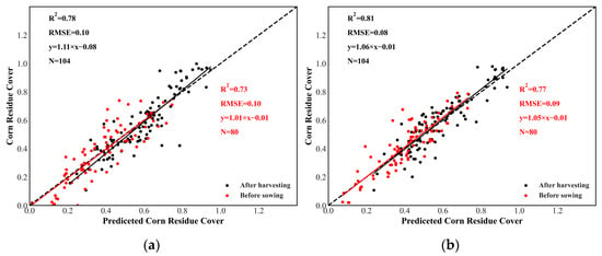
Figure 9.
Estimated result of CRC by multiple linear regression (a) and random forest (b).
Some studies have shown that the relationship between CRC with spectral indices and textural features may be non-linear, which means that the multiple linear regression model cannot capture these complex non-linear relationships [26].Therefore, we explored the potential of the random forest method for CRC estimation, and used the optimal image feature combination type C5 as well. Figure 9b is the estimated accuracy by random forest approach using the optimal image feature combination type C5. The R2 and RMSE both after harvesting and before sowing are 0.81 and 0.08, and 0.77 and 0.09, respectively. Compared with the CRC estimated results using the multiple linear regression approach, the R2 values were all increased and the RMSE values were all decreased using the random forest method. We can conclude that the random forest achieved higher CRC estimation accuracy than the multiple linear regression method with higher R2 values and lower RMSE values both after harvesting and before sowing.
3.5. Contribution of Soil Texture Zoning
The relationship between the spectral index of soil texture after zoning and the measured CRC is shown in Table 6. In different zoning and sampling periods, the performance of each index after zoning improved to a certain extent. Differences in the inverse CRC of the spectral indices between sandy and clayey soil backgrounds and the effect of significant soil heterogeneity on the inverse CRC of the spectral indices are more severe when straw cover is low prior to crop sowing, which reflects the importance of soil zonation modelling.

Table 6.
Determination coefficient between spectral index, texture feature, and CRC of surface soil after texture zoning.
Additionally, we developed the model for CRC estimation in the clayey soil zone and sandy soil zone separately. The CRC estimation models for the two periods after soil texture partitioning are shown in Table 7, from which it can be seen that the accuracy of CRC estimation after partitioning has improved somewhat from before partitioning, reaching an R2 of 0.84 after crop harvesting and 0.81 before sowing using the random forest model. The CRC estimation models based on multiple linear regression models also showed similar accuracy.

Table 7.
Soil texture zoning modelling by different methods.
We assessed the contribution of soil zoning for CRC estimation in this study. Figure 10a is the CRC estimation result using multiple linear regression after soil texture zoning, which shows that the R2 value of CRC estimation after harvesting is 0.81 and RMSE is 0.09, and that the R2 value is 0.76 and RMSE is 0.09 before sowing. Additionally, Figure 10b is the CRC estimation result using a random forest regression after soil texture zoning, which shows that the R2 value of CRC estimation after harvesting is 0.84 and RMSE is 0.08, and that the R2 value is 0.81 and RMSE is 0.09 before sowing. These results reveal that the accuracy of CRC estimation is improved by considering the differences in soil background resulting from soil texture zoning.
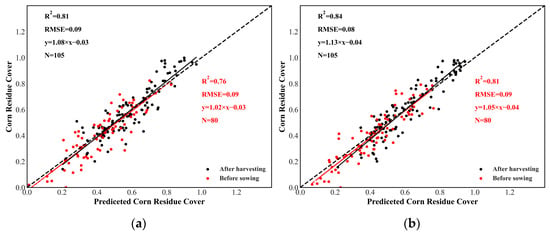
Figure 10.
Estimated result of CRC by multiple linear regression (a) and random forest (b) after soil texture zoning.
3.6. CRC Mapping and Change Monitoring
Using the optimal image feature combination C5, we estimated CRC using the random forest method after soil texture zoning. Additionally, Figure 11 is the estimated CRC result after harvesting and before sowing in the next growing season. The estimated CRC is sorted into three levels: 0~0.3, 0.3~0.6, and 0.6~1.0. According to the definitions provided by the Conservation Technology Information Center (CTIC), the cropland with CRC < 0.3 is considered as conventional tillage and the cropland with CRC > 0.3 is considered as conservation tillage [25]. Figure 11a reveals that there is high corn residue cover in the cropland, with most areas having a coverage of 0.3~0.6 and 0.6~1.0. Quantitatively speaking, 56.16% of the area is covered with a CRC of 0.3~0.6, 34.49% of the area is covered with a CRC greater than 0.6, and only 9.35% of the area is covered with a CRC of less than 0.3 in the whole study area. Regarding the spatial distribution of CRC, the majority is in the SNP plain, which is the major corn-producing region in Northeast China. The second-most corn-residue-covered area is in the LPH plain. Figure 11b is the estimated result of CRC before sowing in the next growing season, and it can be found that most of the area is covered with a CRC of less than 0.3 before sowing. Specifically, 50.63% of the area is covered with a CRC of less than 0.3, 47.89% of the area is covered with a CRC of 0.3~0.6, and only 1.48% of the area is covered with a CRC higher than 0.6. The decrease in CRC after harvesting and before sowing in the next growing season is attributed to the natural decomposition of corn straws and the removal of corn straws for tillage by farmers [25,55].
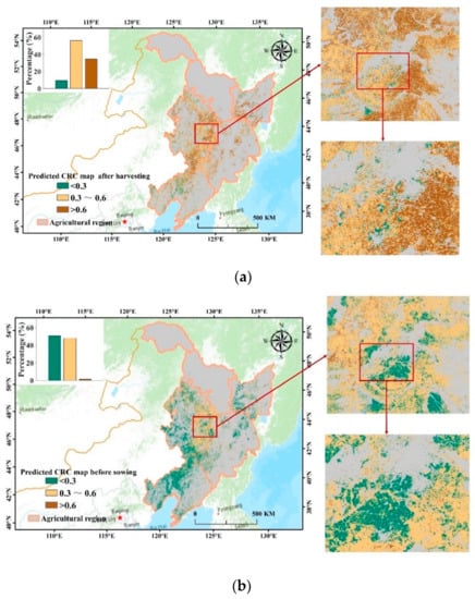
Figure 11.
Predicted CRC map after harvesting (a) and before sowing in the next growing season (b).
4. Discussion
4.1. Feasibility of the CRC Estimation Model
The multiple linear regression and random forest regression methods were used to estimate CRC in this study. Our results in Section 3 reveal that the estimated accuracy using random forest regression is better than that of the multiple linear regression method. We estimated the CRC after harvesting and before sowing in the next growing season using optimized feature combinations and random forest regression. Our results revealed that there is a big difference between the CRC after harvest and before sowing in the next year. Additionally, the CRC value after harvesting was higher than that before sowing in the next growing season [56]. The reasons for this could be that (1) some corn residue may be removed before sowing and (2) the corn residues decompose during the non-growing season. Furthermore, the CRC estimation accuracy after harvesting was higher than that before sowing [29]. Additionally, the reasons for this could be (1) an uneven distribution resulting from the blowing away of residues by strong wind and (2) a greater spectral mixture caused by gradual decomposition.
4.2. Factors Affecting CRC Estimation
The CRC estimation using optical remote sensing images is affected by numerous factors, such as residue moisture content, residue type, soil moisture, and soil roughness [57,58], and this study explores the contribution of soil spatial heterogeneity. The soil types in Northeast China are varied, and there are significant spectral and textural differences between sandy, clayey, and black soil. These differences bring challenges for CRC estimation. In addition to the soil texture, zoning is used to alleviate the effect of soil background, and the shadows of corn residue and soil moisture differences should be considered. Figure 12a shows an example of the mixture of sunlit corn residue, shaded residue, sunlit soil, and shaded soil in one photo taken in the field campaign. Additionally, Figure 12b is an example of corn residue mixed with background soil with high moisture.
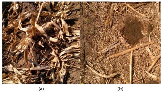
Figure 12.
Examples of corn residue with shadow (a) and with different moisture (b).
Secondly, the temporal mismatch between the image acquisition dates and sample collection dates results in a lower CRC estimation accuracy in the regional area. The Sentinel-2 images with an imaging swath of 290 km, and Landsat-8 images with an imaging swath of 185 km were used for CRC estimation in this study. Considering the cloud and snow coverage, there is only one harmonized image with an obvious time difference that can be found in the whole study area. Furthermore, the corn residue may be decomposed, removed, or burned by the farmer manually. All of these will result in uncertainty for CRC estimation.
5. Conclusions
The CRC estimations after harvesting and before sowing in Northeast China were carried out using Landsat-8 and Sentinel-2 imagery. The optimized combination of image features, a comparison of the random forest and multiple linear regression methods, and a consideration of heterogeneous soil backgrounds were employed for modeling the CRC estimation in different seasons. Regarding the optimization of image features, we found that the combination of spectral indices and texture features can improve the CRC estimation accuracy. Compared with the multiple linear regression approach, the random forest method is more effective with improved accuracy. The R2 between our estimated CRC and measured CRC in the field campaign reaches 0.81 and RMSE is 0.09 using the multiple linear regression approach, and the random forest improves the accuracy, where R2 reaches 0.84 and RMSE is 0.08. These results reveal the potential of CRC estimation modeling by combining spectral indices and textural features by the random forest method in regional areas.
The optimized combination C5 of image features and the random forest was used for CRC mapping. Our estimated results reveal that the CRC is significantly higher after harvesting than before sowing in the next growing season. Additionally, the estimated accuracy after harvesting is higher than that before sowing in the next growing season too. The R2 between our estimated CRC and measured CRC after harvesting reaches 0.84 and RMSE is 0.08. Comparably, R2 reaches 0.81 and RMSE is 0.09 before sowing in the next growing season.
Author Contributions
Conceptualization, data curation, investigation, methodology, formal analysis, writing—original draft, Y.D.; conceptualization, methodology, formal analysis, writing—review and editing, supervision, funding acquisition, W.S.; validation, writing—review and editing, F.X.; project administration, funding acquisition, J.H.; supervision, funding acquisition, W.S.; validation, writing—review and editing, Z.L.; writing—review and editing, X.H.; writing—review and editing, X.L.; supervision, funding acquisition, H.G. All authors have read and agreed to the published version of the manuscript.
Funding
This research was funded by the National Natural Science Foundation of China under the project (No. 42171331), the 2115 Talent Development Program of China Agricultural University.
Data Availability Statement
The data that support the findings of this study were obtained from the Google Earth Engine (https://earthengine.google.com/, accessed on 1 March 2023) and are available from the corresponding author, W.S., upon reasonable request.
Acknowledgments
We appreciate the editors and anonymous reviewers for their valuable time, constructive suggestions, and insightful comments.
Conflicts of Interest
The authors declare no conflict of interest.
References
- Kopittke, P.M.; Menzies, N.W.; Wang, P.; McKenna, B.A.; Lombi, E. Soil and the Intensification of Agriculture for Global Food Security. Environ. Int. 2019, 132, 105078. [Google Scholar] [CrossRef]
- Gerasimova, M. Chinese Soil Taxonomy: Between the American and the International Classification Systems. Eurasian Soil Sci. 2010, 43, 945–949. [Google Scholar] [CrossRef]
- Guo, H.; Zhao, W.; Pan, C.; Qiu, G.; Xu, S.; Liu, S. Study on the Influencing Factors of Farmers’ Adoption of Conservation Tillage Technology in Black Soil Region in China: A Logistic-ISM Model Approach. Int. J. Environ. Res. Public Health 2022, 19, 7762. [Google Scholar] [CrossRef] [PubMed]
- Liu, D.; Wang, Z.; Zhang, B.; Song, K.; Li, X.; Li, J.; Li, F.; Duan, H. Spatial Distribution of Soil Organic Carbon and Analysis of Related Factors in Croplands of the Black Soil Region, Northeast China. Agric. Ecosyst. Environ. 2006, 113, 73–81. [Google Scholar] [CrossRef]
- Najafi, P.; Feizizadeh, B.; Navid, H. A Comparative Approach of Fuzzy Object Based Image Analysis and Machine Learning Techniques Which Are Applied to Crop Residue Cover Mapping by Using Sentinel-2 Satellite and UAV Imagery. Remote Sens. 2021, 13, 937. [Google Scholar] [CrossRef]
- Holland, J.M. The Environmental Consequences of Adopting Conservation Tillage in Europe: Reviewing the Evidence. Agric. Ecosyst. Environ. 2004, 103, 1–25. [Google Scholar] [CrossRef]
- FAO. Food and Agriculture Organization of the United Nations. Available online: https://www.fao.org/conservation-agriculture/en/ (accessed on 2 August 2022).
- Baritz, R.; Wiese-Rozanov, L.; Verbeke, I.; Vargas, R. Voluntary Guidelines for Sustainable Soil Management: Global Action for Healthy Soils. In International Yearbook of Soil Law and Policy; Springer: Berlin/Heidelberg, Germany, 2018; pp. 17–36. ISBN 978-3-319-68884-8. [Google Scholar]
- Gao, L.; Zhang, C.; Yun, W.; Ji, W.; Ma, J.; Wang, H.; Li, C.; Zhu, D. Mapping Crop Residue Cover Using Adjust Normalized Difference Residue Index Based on Sentinel-2 MSI Data. Soil Tillage Res. 2022, 220, 105374. [Google Scholar] [CrossRef]
- Aase, J.K.; Tanaka, D.L. Reflectances from Four Wheat Residue Cover Densities as Influenced by Three Soil Backgrounds. Agron. J. 1991, 83, 753–757. [Google Scholar] [CrossRef]
- Nair, M.; Bherwani, H.; Kumar, S.; Gulia, S.; Goyal, S.; Kumar, R. Assessment of Contribution of Agricultural Residue Burning on Air Quality of Delhi Using Remote Sensing and Modelling Tools. Atmos. Environ. 2020, 230, 117504. [Google Scholar] [CrossRef]
- Rana, M.; Mittal, S.K.; Beig, G.; Rana, P. The Impact of Crop Residue Burning (CRB) on the Diurnal and Seasonal Variability of the Ozone and PM Levels at a Semi-Urban Site in the North-Western Indo-Gangetic Plain. J. Earth Syst. Sci. 2019, 128, 166. [Google Scholar] [CrossRef]
- Daughtry, C.; Hunt, E.R.; Doraiswamy, C.; McMurtrey, J.E. Remote Sensing the Spatial Distribution of Crop Residues. Agron. J. 2005, 97, 864–871. [Google Scholar] [CrossRef]
- Sun, H.; Wang, E.; Li, X.; Cui, X.; Guo, J.; Dong, R. Potential Biomethane Production from Crop Residues in China: Contributions to Carbon Neutrality. Renew. Sustain. Energy Rev. 2021, 148, 111360. [Google Scholar] [CrossRef]
- Tao, W.; Dong, Y.; Su, W.; Li, J.; Xuan, F.; Huang, J.; Yang, J.; Li, X.; Zeng, Y.; Li, B. Mapping the Corn Residue-Covered Types Using Multi-Scale Feature Fusion and Supervised Learning Method by Chinese GF-2 PMS Image. Front. Plant Sci. 2022, 13, 901042. [Google Scholar] [CrossRef] [PubMed]
- Zhang, M.; Li, Q.; Meng, J.; Wu, B. Review of Crop Residue Fractional Cover Monitoring with Remote Sensing. Spectrosc. Spectr. Anal. 2011, 31, 3200–3205. [Google Scholar]
- Pacheco, A.; McNairn, H. Evaluating Multispectral Remote Sensing and Spectral Unmixing Analysis for Crop Residue Mapping. Remote Sens. Environ. 2010, 114, 2219–2228. [Google Scholar] [CrossRef]
- Zhou, D.; Li, M.; Li, Y.; Qi, J.; Liu, K.; Cong, X.; Tian, X. Detection of Ground Straw Coverage under Conservation Tillage Based on Deep Learning. Comput. Electron. Agric. 2020, 172, 105369. [Google Scholar] [CrossRef]
- Najafi, P.; Navid, H.; Feizizadeh, B.; Eskandari, I. Object-Based Satellite Image Analysis Applied for Crop Residue Estimating Using Landsat OLI Imagery. Int. J. Remote Sens. 2018, 39, 6117–6136. [Google Scholar] [CrossRef]
- Nagler, P.L.; Daughtry, C.S.T.; Goward, S.N. Plant Litter and Soil Reflectance. Remote Sens. Environ. 2000, 71, 207–215. [Google Scholar] [CrossRef]
- Daughtry, C. Discriminating Crop Residues from Soil by Shortwave Infrared Reflectance. Agron. J. 2001, 93, 125–131. [Google Scholar] [CrossRef]
- Van Deventer, A.P.; Ward, A.D.; Gowda, P.H.; Lyon, J.G. Using Thematic Mapper Data to Identify Contrasting Soil Plains and Tillage Practices. Photogramm. Eng. Remote Sens. 1997, 63, 87–93. [Google Scholar]
- Quemada, M.; Menacho, E. Soil Respiration 1 Year after Sewage Sludge Application. Biol. Fertil. Soils 2001, 33, 344–346. [Google Scholar] [CrossRef]
- Yue, J.; Tian, Q.; Dong, X.; Xu, K.; Zhou, C. Using Hyperspectral Crop Residue Angle Index to Estimate Maize and Winter-Wheat Residue Cover: A Laboratory Study. Remote Sens. 2019, 11, 807. [Google Scholar] [CrossRef]
- Xiang, X.; Du, J.; Jacinthe, P.-A.; Zhao, B.; Zhou, H.; Liu, H.; Song, K. Integration of Tillage Indices and Textural Features of Sentinel-2A Multispectral Images for Maize Residue Cover Estimation. Soil Tillage Res. 2022, 221, 105405. [Google Scholar] [CrossRef]
- Ding, Y.; Zhang, H.; Wang, Z.; Xie, Q.; Wang, Y.; Liu, L.; Hall, C.C. A Comparison of Estimating Crop Residue Cover from Sentinel-2 Data Using Empirical Regressions and Machine Learning Methods. Remote Sens. 2020, 12, 1470. [Google Scholar] [CrossRef]
- Yue, J.; Tian, Q. Estimating Fractional Cover of Crop, Crop Residue, and Soil in Cropland Using Broadband Remote Sensing Data and Machine Learning. Int. J. Appl. Earth Obs. Geoinf. 2020, 89, 102089. [Google Scholar] [CrossRef]
- Sun, Z.; Zhu, Q.; Deng, S.; Li, X.; Hu, X.; Chen, R.; Shao, G.; Yang, H.; Yang, G. Estimation of Crop Residue Cover in Rice Paddies by a Dynamic-Quadripartite Pixel Model Based on Sentinel-2A Data. Int. J. Appl. Earth Obs. Geoinf. 2022, 106, 102645. [Google Scholar] [CrossRef]
- Tao, W.; Xie, Z.; Zhang, Y.; Li, J.; Xuan, F.; Huang, J.; Li, X.; Su, W.; Yin, D. Corn Residue Covered Area Mapping with a Deep Learning Method Using Chinese GF-1 B/D High Resolution Remote Sensing Images. Remote Sens. 2021, 13, 2903. [Google Scholar] [CrossRef]
- You, N.; Dong, J.; Huang, J.; Du, G.; Zhang, G.; Yingli, H.; Yang, T.; Di, Y.; Xiao, X. The 10-m Crop Type Maps in Northeast China during 2017–2019. Sci. Data 2021, 8, 41. [Google Scholar] [CrossRef]
- Liu, W.; Dong, J.; Du, G.; Zhang, G.; Hao, Z.; You, N.; Zhao, G.; Flynn, K.C.; Yang, T.; Zhou, Y. Biophysical Effects of Paddy Rice Expansion on Land Surface Temperature in Northeastern Asia. Agric. For. Meteorol. 2022, 315, 108820. [Google Scholar] [CrossRef]
- Otsu, N. A Threshold Selection Method from Gray-Level Histograms. IEEE Trans. Syst. Man Cybern. 1979, 9, 62–66. [Google Scholar] [CrossRef]
- Bastin, J.-F.; Berrahmouni, N.; Grainger, A.; Maniatis, D.; Mollicone, D.; Moore, R.; Patriarca, C.; Picard, N.; Sparrow, B.; Abraham, E.M.; et al. The Extent of Forest in Dryland Biomes. Science 2017, 356, 635–638. [Google Scholar] [CrossRef] [PubMed]
- Chastain, R.; Housman, I.; Goldstein, J.; Finco, M.; Tenneson, K. Empirical Cross Sensor Comparison of Sentinel-2A and 2B MSI, Landsat-8 OLI, and Landsat-7 ETM+ Top of Atmosphere Spectral Characteristics over the Conterminous United States. Remote Sens. Environ. 2019, 221, 274–285. [Google Scholar] [CrossRef]
- Beeson, P.C.; Daughtry, C.S.T.; Wallander, S.A. Estimates of Conservation Tillage Practices Using Landsat Archive. Remote Sens. 2020, 12, 2665. [Google Scholar] [CrossRef]
- McNairn, H.; Protz, R. Mapping Corn Residue Cover on Agricultural Fields in Oxford County, Ontario, Using Thematic Mapper. Can. J. Remote Sens. 1993, 19, 152–159. [Google Scholar] [CrossRef]
- Qi, J.; Marsett, R.; Heilman, P.; Bieden-bender, S.; Moran, S.; Goodrich, D.; Weltz, M. RANGES Improves Satellite-Based Information and Land Cover Assessments in Southwest United States. Eos Trans. Am. Geophys. Union 2002, 83, 601–606. [Google Scholar] [CrossRef]
- Sullivan, D.G.; Truman, C.; Schomberg, H.; Endale, D.; Strickland, T. Evaluating Techniques for Determining Tillage Regime in the Southeastern Coastal Plain and Piedmont. Agron. J. 2006, 98, 1236–1246. [Google Scholar] [CrossRef]
- Gelder, B.K.; Kaleita, A.L.; Cruse, R.M. Estimating Mean Field Residue Cover on Midwestern Soils Using Satellite Imagery. Agron. J. 2009, 101, 635–643. [Google Scholar] [CrossRef]
- Haralick, R.; Shanmugam, K.; Dinstein, I. Textural Features for Image Classification. IEEE Trans. Syst. Man Cybern. 1973, 6, 610–621. [Google Scholar] [CrossRef]
- Barber, D.; LeDrew, E. SAR Sea Ice Discrimination Using Texture Statistics: A Multivariate Approach. Photogramm. Eng. Remote Sens. 1991, 57, 385–395. [Google Scholar]
- Soh, L.-K.; Tsatsoulis, C. Texture Analysis of SAR Sea Ice Imagery Using Gray Level Co-Occurrence Matrices. IEEE Trans. Geosci. Remote Sens. 1999, 37, 780–795. [Google Scholar] [CrossRef]
- Su, W.; Zhang, C.; Yang, J.; Wu, H.; Deng, L.; Ou, W.; Yue, A.; Chen, M. Analysis of Wavelet Packet and Statistical Textures for Object-Oriented Classification of Forest-Agriculture Ecotones Using SPOT 5 Imagery. Int. J. Remote Sens. 2012, 33, 3557–3579. [Google Scholar] [CrossRef]
- Wood, E.M.; Pidgeon, A.M.; Radeloff, V.C.; Keuler, N.S. Image Texture as a Remotely Sensed Measure of Vegetation Structure. Remote Sens. Environ. 2012, 121, 516–526. [Google Scholar] [CrossRef]
- Su, W.; Li, J.; Chen, Y.; Liu, Z.; Zhang, J.; Low, T.; Suppiah, I.; Hashim, A. Textural and Local Spatial Statistics for the Object-Oriented Classification of Urban Areas Using High Resolution Imagery. Int. J. Remote Sens. 2008, 29, 3105–3117. [Google Scholar] [CrossRef]
- Olson, K.; White, R.; Sindelar, B. Response of Vegetation of the Northern Great Plains to Precipitation Amount and Grazing Intensity. J. Range Manag. 1985, 38, 357–361. [Google Scholar] [CrossRef]
- Breiman, L. Random Forests. Mach. Learn. 2001, 45, 5–32. [Google Scholar] [CrossRef]
- Mutanga, O.; Adam, E.; Cho, M.A. High Density Biomass Estimation for Wetland Vegetation Using WorldView-2 Imagery and Random Forest Regression Algorithm. Int. J. Appl. Earth Obs. Geoinf. 2012, 18, 399–406. [Google Scholar] [CrossRef]
- Liu, Z.; Wan, W.; Huang, J.; Wang, J.; Zheng, M. Estimation of maize residue cover on the basis of SAR and optical remote sensing image. Natl. Remote Sens. Bull. 2021, 25, 1308–1323. [Google Scholar]
- Jin, X.; Xu, X.; Song, X.; Li, Z.; Wang, J.; Guo, W. Estimation of Leaf Water Content in Winter Wheat Using Grey Relational Analysis–Partial Least Squares Modeling with Hyperspectral Data. Agron. J. 2013, 105, 1385–1392. [Google Scholar] [CrossRef]
- Xuan, F.; Dong, Y.; Li, J.; Li, X.; Su, W.; Huang, X.; Huang, J.; Xie, Z.; Li, Z.; Liu, H.; et al. Mapping Crop Type in Northeast China during 2013–2021 Using Automatic Sampling and Tile-Based Image Classification. Int. J. Appl. Earth Obs. Geoinf. 2023, 117, 103178. [Google Scholar] [CrossRef]
- Berberoglu, S.; Lloyd, C.D.; Atkinson, P.M.; Curran, P.J. The Integration of Spectral and Textural Information Using Neural Networks for Land Cover Mapping in the Mediterranean. Comput. Geosci. 2000, 26, 385–396. [Google Scholar] [CrossRef]
- Zhou, J.-J.; Zhao, Z.; Zhao, J.; Zhao, Q.; Wang, F.; Wang, H. A Comparison of Three Methods for Estimating the LAI of Black Locust (Robinia pseudoacacia L.) Plantations on the Loess Plateau, China. Int. J. Remote Sens. 2014, 35, 171–188. [Google Scholar] [CrossRef]
- Jin, X.; Ma, J.; Wen, Z.; Song, K. Estimation of Maize Residue Cover Using Landsat-8 OLI Image Spectral Information and Textural Features. Remote Sens. 2015, 7, 14559–14575. [Google Scholar] [CrossRef]
- Wan, W.; Liu, Z.; Li, B.; Fang, H.; Wu, H.; Yang, H. Evaluating Soil Erosion by Introducing Crop Residue Cover and Anthropogenic Disturbance Intensity into Cropland C-Factor Calculation: Novel Estimations from a Cropland-Dominant Region of Northeast China. Soil Tillage Res. 2022, 219, 105343. [Google Scholar] [CrossRef]
- Zhang, Z.; Qiang, H.; McHugh, A.D.; He, J.; Li, H.; Wang, Q.; Lu, Z. Effect of Conservation Farming Practices on Soil Organic Matter and Stratification in a Mono-Cropping System of Northern China. Soil Tillage Res. 2016, 156, 173–181. [Google Scholar] [CrossRef]
- Serbin, G.; Daughtry, C.S.T.; Hunt, E.R.; Reeves, J.B.; Brown, D.J. Effects of Soil Composition and Mineralogy on Remote Sensing of Crop Residue Cover. Remote Sens. Environ. 2009, 113, 224–238. [Google Scholar] [CrossRef]
- Quemada, M.; Hively, W.D.; Daughtry, C.S.T.; Lamb, B.T.; Shermeyer, J. Improved Crop Residue Cover Estimates Obtained by Coupling Spectral Indices for Residue and Moisture. Remote Sens. Environ. 2018, 206, 33–44. [Google Scholar] [CrossRef]
Disclaimer/Publisher’s Note: The statements, opinions and data contained in all publications are solely those of the individual author(s) and contributor(s) and not of MDPI and/or the editor(s). MDPI and/or the editor(s) disclaim responsibility for any injury to people or property resulting from any ideas, methods, instructions or products referred to in the content. |
© 2023 by the authors. Licensee MDPI, Basel, Switzerland. This article is an open access article distributed under the terms and conditions of the Creative Commons Attribution (CC BY) license (https://creativecommons.org/licenses/by/4.0/).